Before You Start

Some of the math in these notes does not render correctly in Safari. I haven't tested it on any of the Microsoft-specific browsers. It is recommended that you view these notes in Firefox or Chrome.

Given the tools I use to generate these notes, I have little control over the scroll position of an anchor referenced by a link. Thus, when you follow a link, the referenced element will almost always appear just above the visible portion of the page. Remember to scroll up. I need to figure out a way to fix this, but right now finishing these notes is more important.

The material in these notes goes beyond what we cover in class. Sections that are marked with a star (*) are not covered in class; you can read them if you wish, and I am more than happy to discuss the material they cover with you, but you are not required to read them. The sections that are not marked are material we cover in class.

Some of the figures contain a lot of information and are scaled down to fit the width of a text column. If you hover the mouse over any figure, it gets scaled up, so figures should become easier to read.

1. Overview

1.1. Topics Covered

A one-semester course on advanced algorithms is necessarily incomplete, both in terms of the choice of topics covered and in terms of the depth in which it covers the topics that it does cover. I chose the topics for this course based on two criteria: First, the studied problems should have practical relevance, where "practical" is to be interpreted quite generally; the algorithms should be useful either for tackling problems arising in real-world applications or as building blocks for other algorithms. Second, the techniques used in developing these algorithms should be interesting and instructive. Based on these two criteria, there are three major themes this course will cover.

Advanced graph algorithms are used as building blocks of many other algorithms. It is amazing how many problems reduce to network flow or matching problems. So the first part of the course focuses on studying efficient algorithms for these problems. Before covering advanced graph algorithms, we discuss (integer) linear programming because it is a useful tool for modelling a wide range of optimization problems and is used as a building block for some of the algorithms discussed in this class.

Classical algorithm theory views NP-hardness as a "death sentence" for a problem in the sense that no "efficient" (i.e., polynomial-time) algorithm for such a problem is likely to exist. This view is too limited for at least two reasons: First, advances in the design of algorithms have led to very efficient solutions to many NP-hard problems, albeit obviously not polynomial-time solutions. Remember that polynomial time is just an approximation of efficiency; there exist very inefficient polynomial-time algorithms and rather efficient exponential-time algorithms. Second, there is a great need for algorithms that solve NP-hard problems because an increasing number of application areas give rise to a wealth of NP-hard problems that simply need to be solved. The second part of this course thus focuses on techniques for coping with NP-hardness. This part is divided into two components. The first one is concerned with approximation algorithms. If an optimization problem is NP-hard, we should not hope to find an optimal solution in polynomial time. However, what if an approximate solution is good enough in a particular application? How well can the optimal solution be approximated in polynomial time? This is the central question answered by the theory of approximation algorithms. The second component covers two types of algorithms that both find exact answers to NP-hard problems and thus necessarily take exponential time. Just as a linear-time algorithm is preferable over a quadratic-time algorithm, even though both take polynomial time, an \(O\bigl(1.1^n\bigr)\)-time algorithm is obviously much better than one that takes \(O\bigl(4^n\bigr)\) time. Exact exponential algorithms have the goal to achieve the fastest possible exponential running time for solving an NP-hard problem. Fixed-parameter algorithms go a step further in that they aim to achieve a running time that is polynomial in the input size and exponential only in some hardness parameter of the input; for an NP-hard problem, this hardness parameter must be linear in the input size for some inputs, but the hope is that for many inputs, particularly those arising in certain applications, the parameter is much smaller than \(n\). Since there is a lot of overlap between the techniques used in designing exact exponential algorithms and fixed-parameter algorithms, we discuss them together.

There are a number of topics that fully deserve to be covered in this course but which I chose not to cover:

Advanced data structures. Almost all non-trivial algorithms rely on support from good data structures, so data structures are of tremendous importance. There is a simple reason why advanced data structures are not a major focus of this course: Meng He already offers an advanced data structures course, which you are strongly encouraged to take.

Parallel algorithms. Multicore processors and massively parallel systems based on cloud architectures or GPUs have become ubiquitous. Designing parallel algorithms for such systems poses a whole new layer of challenges that are of no concern when designing traditional, sequential algorithms. Once again, parallel algorithms are not a focus of this course because there already is a parallel computing course in our Faculty. Designing efficient parallel algorithms can require a very different way of thinking about problem decomposition than when designing sequential algorithms. You are strongly encouraged to take the parallel computing course to learn about these questions.

Computational geometry. This is probably the least justified omission. Computational geometry is a treasure trove of interesting problems and techniques to solve them. Many widely applicable data structuring techniques were developed in the context of developing data structures for geometric problems. However, it would be simply impossible to cover graph algorithms, approximation and exact exponential algorithms, and computational geometry in the same course without reducing the exposition of each topic to a mere scratch of the surface. In my personal opinion, network flows, cuts, and matchings are more fundamental, with a wider range of applications than many geometric algorithms, and coming to terms with NP-hardness also seems to be of tremendous importance nowadays. So, purely subjectively, I decided not to cover geometric algorithms in this course, even though computational geometry is full of beautiful ideas and algorithms based on them.

Memory hierarchies. While today's processors have the computing power of supercomputers of the 1980s, memory access speeds have not increased nearly as fast. As a result, it is challenging to supply modern CPUs with data at the rate at which they can process it. To bridge the widening gap between processor and memory speeds, modern computers have a memory hierarchy consisting of several layers of cache, RAM, and hard disks or SSDs. The farther away a memory level is from the CPU, the larger it is, but its access cost also increases. To amortize addressing costs, data is transferred between adjacent levels in blocks of a certain size. If algorithms have high access locality, this is an effective strategy to alleviate the bottleneck posed by RAM and disk accesses. Designing algorithms with locality of access, on the other hand, is extremely challenging for some problems and, even for problems where such efforts were successful, the required techniques often depart significantly from the ones used in classical algorithms, in a manner similar to parallel algorithms. I used to teach an entire course on algorithms for memory hierarchies since this was my main research area. Not talking about algorithms for memory hierarchies in this course was another sacrifice I had to make in order to be able to cover the topics I do cover in sufficient depth.

Online algorithms. Most of the time when we talk about algorithms, we assume that the entire input is given to the algorithm in one piece. The algorithm can analyze this input any way it wants, in order to compute the desired solution as efficiently as possible. There are applications, however, where this assumption is not satisfied. Paging, the process of deciding which data items to keep in cache, is one such example: When a page is requested that is not in cache, it is brought into cache and the algorithm has to make a decision which page to evict from the cache in order to make room for it. The choice of the evicted page can have significant impact on the cost of future memory accesses, so it would be nice to know all future memory accesses. However, this information is simply not available, so we have to make the best possible decision with the information we have available at the time it needs to be made. There are numerous other problems of the same flavour. The theory and practice of online algorithms studies how good approximations to an optimal solution can be computed in such a scenario. Again, there are many beautiful ideas that were developed to obtain such algorithms. Not covering them was again a trade-off I made in order to cover the topics I do cover in sufficient depth.

Streaming algorithms. These algorithms are closely related to online algorithms and I/O-efficient algorithms. Where I/O-efficient algorithms try to alleviate the I/O bottleneck by being careful about how they access the hard drive in computations on data sets beyond the size of the computer's RAM, streaming algorithms completely eliminate the I/O bottleneck by processing data as it arrives (similarly to online algorithms) and only storing as much information about the data elements seen so far as fits in memory. As is the case for online algorithms, this raises the question of how good approximations of the correct answer to a given problem can be computed in this fashion. There is a simple reason why streaming algorithms are not covered in this course: I do not know enough about them (yet).

1.2. Prerequisites

A discussion of advanced algorithms needs as a foundation a solid understanding of basic algorithmic concepts, as covered in CSCI 3110.

In terms of specific problems and algorithms to solve them, the prerequisites for this course are fairly modest. I assume that you know about sorting, selection, and binary search and understand the algorithms that solve these problems. I also expect you to know about basic graph traversals (BFS and DFS), their cost, and the type of problems they can be used to solve. Finally, I assume that you know what a minimum spannning tree or shortest path tree is, along with algorithms to compute them (Bellman-Ford, Ford-Fulkerson, Dijkstra, Prim, Kruskal). Any other algorithms needed as building blocks of algorithms discussed in this course are introduced as needed.

I assume a greater degree of preparedness in terms of your comfort with simply talking about algorithmic problems. You should have a solid understanding of and be able to comfortably work with \(O\)-, \(\Omega\)-, \(\Theta\)-, \(o\)-, and \(\omega\)-notation and you should have an appreciation for the need for formalism and rigour in describing algorithms and in arguing about their correctness and running times. Having said that, I will often appeal to your intuition about various algorithmic questions and will implicitly assume that you are able to translate this intuition into formal arguments.

As far as algorithmic techniques go, divide and conquer should be your bread and butter and you should be comfortable with greedy algorithms and dynamic programming, as they will be used extensively in this course to solve various subproblems in approximate and exact solutions to NP-hard problems.

If you cannot put a checkmark beside each of these topics, now is the time to open your CSCI 3110 textbook (most likely Cormen et al. or Kleinberg/Tardos) and refresh your memory on these topics.

1.3. A Note on Graphs

Many of the problems studied in this course are graph problems, because almost anything can be modelled as a graph problem. For some of these problems, it is important whether the underlying graph is directed or undirected; for others, it is irrelevant beyond the fact that, in a directed graph, the two edges \((v,w)\) and \((w,v)\) are separate entities while they are the same in an undirected graph. For problems that can be defined for both directed and undirected graph, I will simply use the term "graph", without specifying whether it is directed or undirected. You should check in these cases that the problem definition and the developed algorithms are indeed sound both if the graph is undirected and if it is directed. When it is important whether the graph is directed or undirected, I state this explicitly.

2. Linear Programming

Linear programming (LP), as a tool for modelling optimization problems and as an algorithmic problem to be solved efficiently, can easily fill an entire course. Since this course focuses mainly on combinatorial algorithms for a wide range of problems, we do not cover LP in much depth. However, many of the problems discussed in this course have elegant LP or integer linear programming (ILP) formulations that shed light on the structure of the problems, and some of the developed algorithms use linear programming as a building block. Thus, a basic understanding of LP and ILP and of the basic techniques to solve LP and ILP problems is important for later topics covered in this course.

The discussion of LPs is split into three parts. In this chapter, we introduce what linear programs and integer linear programs are, and how to use them to model optimization problems. Chapter 3 introduces a classical algorithm for solving linear programs, the Simplex Algorithm. The proof of correctness of this algorithm is deferred to Chapter 4, which introduces LP duality and complementary slackness as two central tools for proving that a given solution of an LP is optimal.

The roadmap for this chapter is as follows:

• Section 2.1 defines what a linear program is.

• Section 2.2 illustrates the use of linear programs to model optimization problems using the single-source shortest paths problem as an example.

• Section 2.3 introduces integer linear programming and illustrates its usefulness as a tool for modelling optimization problems by showing how to convert the minimum spanning tree problem into an ILP.

• Section 2.4 explores the computational complexity of linear programming and integer linear programming. Linear programs can be solved in polynomial time, often even if they have an exponential number of constraints. Integer linear programming, on the other hand, is NP-hard. This raises the question whether we can use the tools to solve linear programs efficiently also to obtain good, albeit not optimal, solutions of ILPs.

• Section 2.5 discusses LP relaxations as a way to convert an ILP into a related LP. LP relaxation plays an important role in approximation algorithms, discussed in the third part of this book.

• Section 2.6 finally, discusses two commonly used forms of linear programs. One of them—canonical form—plays a key role in the theory of LP duality. The other—standard form—is the input expected by the Simplex Algorithm.

2.1. Linear Programs

A linear program (LP) \(P\) is an optimization problem over a set of real-valued variables \(\{x_1, \ldots, x_n\}\). We usually represent this set of variables as a vector \(x = (x_1, \ldots, x_n)\). Its description includes a linear objective function \(f(x_1, \ldots, x_n)\) and a collection of \(m\) linear constraints, that is, linear inequalities involving the variables \(x_1, \ldots, x_n\). The goal is to find an assignment of real values \({\hat x} = (\hat x_1, \ldots, \hat x_n)\) to the variables in \(x = (x_1, \ldots, x_n)\) that satisfies all constraints in \(P\) and either minimizes or maximizes the objective function value \(f(\hat x_1, \ldots, \hat x_n)\). Whether a minimum or maximum objective function value is sought is part of the problem description and the problem is accordingly called a minimization LP or a maximization LP. An assignment \(\hat x\) that minimizes or maximizes the objective function value subject to the given set of linear constraints is called an optimal solution of the LP \(P\). If \(\hat x\) satisfies the constraints in \(P\) but may or may not maximize \(f(\hat x_1, \ldots, \hat x_n)\), then \(\hat x\) is called a feasible solution of \(P\).

Reading \((\hat x_1, \ldots, \hat x_n)\) as an \(n\)-dimensional vector, the set of feasible solutions for a single linear constraint is always a halfspace, the portion of \(\mathbb{R}^n\) on one side of an \((n-1)\)-dimensional hyperplane. This is called the feasible region of the constraint. Since a feasible solution for a set of constraints must satisfy every constraint in the set, the feasible region of the constraints in \(P\) is the intersection of the feasible regions of the individual constraints and is thus convex. This convexity, together with the linearity of the constraints and objective function is the key to solving linear programs efficiently.

As an example, consider the following linear program over two variables \(x\) and \(y\):

\[\begin{gathered} \text{Maximize } x + 2y\\ \begin{aligned} \text{s.t. (subject to) } \hphantom{3x + y} \llap{x} &\ge 0\\ y &\ge 0\\ 3x + y &\le 26\\ 4x - y &\le 31\\ 2y - x &\le 4 \end{aligned} \end{gathered}\tag{2.1}\]

The constraints and feasible region of (2.1) are shown in Figure 2.1. The optimal solution is the red point \(\bigl(\frac{48}{7}, \frac{38}{7}\bigr)\) with objective function value \(\frac{48}{7} + 2 \cdot \frac{38}{7} = \frac{124}{7}\).

Figure 2.1: The feasible region of the constraint \(3x + y \le 26\) is shaded light blue. The feasible region of the set of all constraints in (2.1) is shaded light red. The red dot is the optimal solution of (2.1). All solutions on each of the blue lines have the same objective function value. Moving in the direction indicated by the red arrow increases the objective function value.

The fact that, in this example, the optimal solution is a vertex of the feasible region is not a coincidence. Since moving the solution in a particular direction (the red arrow in Figure 2.1) increases the objective function, the maximum objective function value is always obtained at a point on the boundary of the feasible region. If this point is not a vertex of the feasible region, it is an interior point of a boundary facet of the feasible region (a segment in 2-d, an up to \((n-1)\)-dimensional convex region in higher dimensions), and every point in this facet has the same objective function value. Thus, the solution can be moved to a boundary vertex of this facet without changing the objective function value; this boundary vertex of this facet is a boundary vertex of the feasible region. The Simplex Algorithm exploits the fact that only vertices of the feasible region need to be considered in the search for an optimal solution.

2.2. Shortest Paths as an LP

2.2.1. The Single-Source Shortest Paths Problem

As a first example of the use of linear programs to model optimization problems, consider the single-source shortest paths problem.

Given a graph \(G = (V, E)\), a path from a vertex \(s\) to a vertex \(t\) is a sequence of vertices \(P = \langle v_0, \ldots, v_k \rangle\) such that \(v_0 = s\), \(v_k = t\), and there exists an edge \(e_i = (v_{i-1},v_i) \in E\) for all \(1 \le i \le k\). See Figure 2.2.

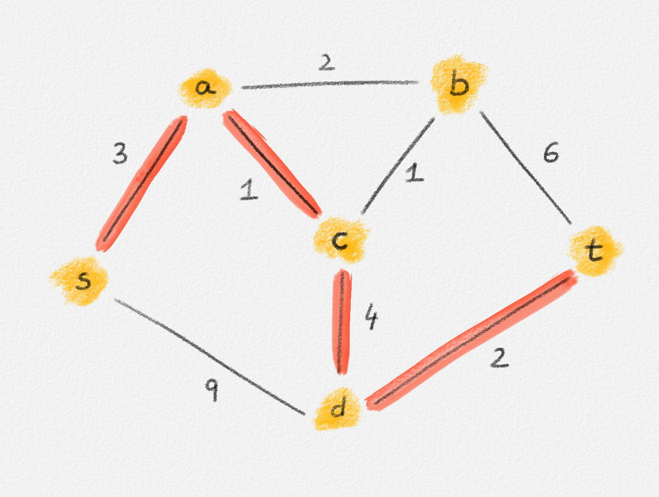
Figure 2.2: The red path \(\langle s, a, c, d, t\rangle\) is a shortest path from \(s\) to \(t\) of length \(10\). \(\langle s, d, t\rangle\) is another path from \(s\) to \(t\), but it is not a shortest path because its length is \(11\).

Depending on the context, \(P\) may be viewed as the sequence of its vertices, the sequence of its edges \(\langle e_1, \ldots, e_k \rangle\) or the alternating sequence of both \(\langle v_0, e_1, v_1, \ldots, e_k, v_k \rangle\).

A path \(P\) from a vertex \(s\) to a vertex \(t\) is a cycle if \(s = t\). See Figure 2.3.

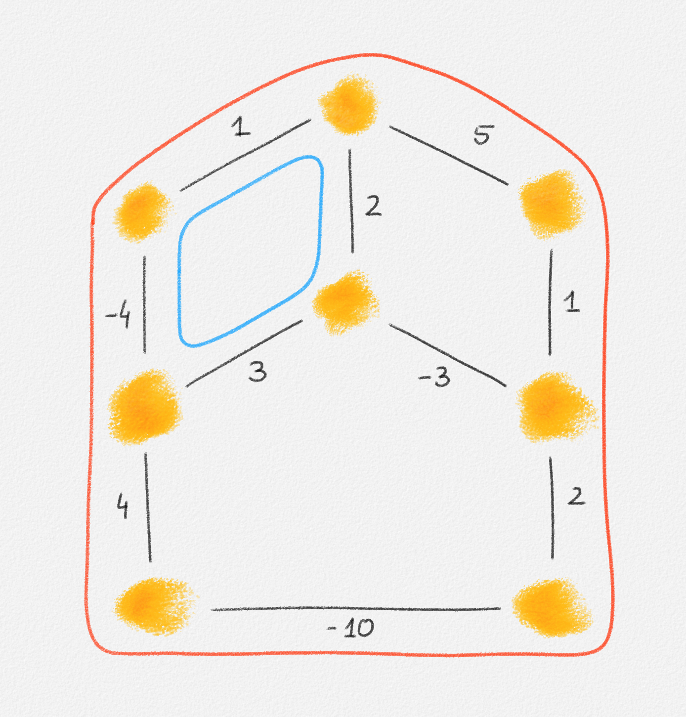
Figure 2.3: The red and blue paths are cycles. The red one is a negative cycle of weight \(-1\). The blue one is not a negative cycle; its weight is \(2\).

An edge-weighted graph is a pair \((G,w)\) consisting of a graph \(G = (V,E)\) and an assignment \(w : E \rightarrow \mathbb{R}\) of weights to its edges.

The weight or length of a path \(P\) in an edge-weighted graph \((G,w)\) is the total weight of all edges in \(P\):

\[w(P) = \sum_{e \in P} w_e\]

A shortest path from a vertex \(s \in V\) to a vertex \(t \in V\) is a path \(\Pi_{G,w}(s,t)\) from \(s\) to \(t\) in \(G\) such that every path \(P\) from \(s\) to \(t\) in \(G\) satisfies \(w(P) \ge w(\Pi_{G,w}(s,t))\).

The distance from \(s\) to \(t\) is

\[\mathrm{dist}_{G,w}(s,t) = w(\Pi_{G,w}(s,t)).\]

Shortest paths in an edge-weighted graph \((G,w)\) are well defined only if there are no negative cycles in \((G,w)\), where

A negative cycle is a cycle \(C\) in \(G\) with \(w(C) < 0\).

Indeed, if there exists a path from \(s\) to \(t\) that includes a vertex in some negative cycle \(C\), then it is possible to generate arbitrarily short paths from \(s\) to \(t\) by including sufficiently many passes through \(C\) in the path.

The single-source shortest paths problem is to compute the distance from some source vertex \(s\) to every vertex \(v \in V\):

Single-source shortest paths problem (SSSP): For an edge-weighted graph \((G,w)\) and a source vertex \(s \in V\), compute \(\mathrm{dist}_{G,w}(s, v)\) for all \(v \in V\).

In general, the goal is to find the actual shortest paths \(\Pi_{G,w}(s,v)\), not only the distances \(\mathrm{dist}_{G,w}(s,v)\). By the following two exercises, computing the distances is the hard part.

Exercise 2.1: In general, there may be more than one shortest path between two vertices \(s\) and \(t\) in a connected edge-weighted graph \((G, w)\). Prove that it is possible to choose a particular shortest path \(\Pi_{G,w}(s, v)\) for each vertex \(v \in V\) such that the union of these shortest paths is a tree. This tree is called a shortest path tree.

Exercise 2.2: Show that finding the shortest paths from a vertex \(s\) to all vertices \(v\) in an edge-weighted graph \((G, w)\) is no harder than computing the distances from \(s\) to all vertices in \(G\). Specifically, if \(d : V \rightarrow \mathbb{R}\) is a labelling of the vertices of \(G\) such that \(d_v = \mathrm{dist}_{G,w}(s,v)\) for all \(v \in V\), show how to compute a shortest path tree \(T\) with root \(s\) in \(O(n + m)\) time.

2.2.2. Properties of Shortest Paths

The LP formulation of the SSSP problem is based on the following two properties of distances from \(s\).

Lemma 2.1: Let \(v \ne s\) and let \(u\) be \(v\)'s predecessor in \(\Pi_{G,w}(s,v)\). Then the subpath \(P\) of \(\Pi_{G,w}(s,v)\) from \(s\) to \(u\) is a shortest path from \(s\) to \(u\).

Proof: Since \(P\) is a path from \(s\) to \(u\), we have

\[w(P) \ge \mathrm{dist}_{G,w}(s,u).\]

If \(w(P) > \mathrm{dist}_{G,w}(s,u)\), then the path \(\Pi_{G,w}(s,u) \circ \langle (u,v) \rangle\) (the concatenation of the path \(\Pi_{G,w}(s,u)\) with the single-edge path \(\langle (u,v) \rangle\)) is a path from \(s\) to \(v\) of length

\[\mathrm{dist}_{G,w}(s,u) + w_{u,v} < w(P) + w_{u,v} = \mathrm{dist}_{G,w}(s,v),\]

a contradiction. This is illustrated in Figure 2.4. ▨

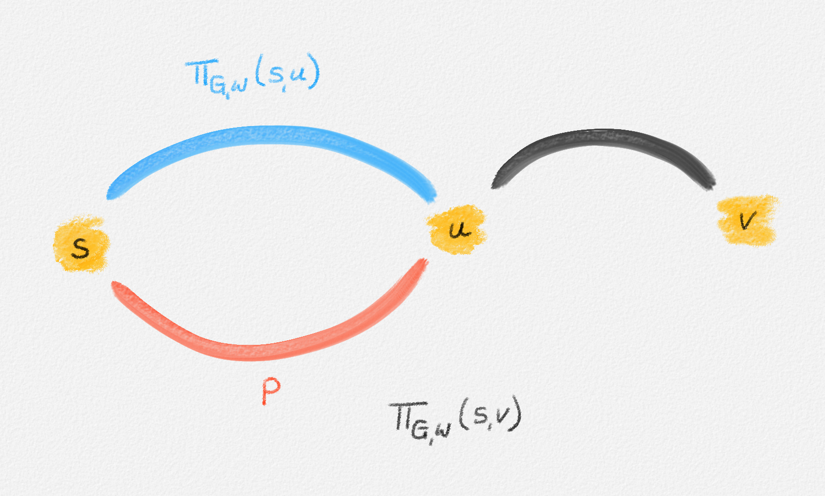
Figure 2.4: If \(\Pi_{G,w}(s,u)\) is shorter than \(P\), then \(\Pi_{G,w}(s,v)\) cannot be a shortest path.

Lemma 2.2:

\[\begin{multline} \mathrm{dist}_{G,w}(s,v) =\\ \begin{cases} 0 & \text{if } v = s\\ \min \{ \mathrm{dist}_{G,w}(s,u) + w_{u,v} \mid (u,v) \in E \} & \text{if } v \ne s \end{cases}\phantom{spc} \end{multline}\tag{2.2}\]

Proof: The case when \(v = s\) is obvious since the shortest path from \(s\) to \(s\) contains only \(s\) and thus has length \(0\). (Convince yourself that this follows from the absence of negative cycles.)

For \(v \ne s\), let \(z\) be \(v\)'s predecessor in \(\Pi_{G,w}(s,v)\). By Lemma 2.1,

\[\begin{aligned} \mathrm{dist}_{G,w}(s,v) &= \mathrm{dist}_{G,w}(s,z) + w_{z,v}\\ &\ge \min \{ \mathrm{dist}_{G,w}(s,u) + w_{u,v} \mid (u,v) \in E \}. \end{aligned}\tag{2.3}\]

Conversely, if \(z'\) is \(v\)'s in-neighbour that minimizes \(\mathrm{dist}_{G,w}(s,z') + w_{z',v}\), then \(\Pi_{G,w}(s, z') \circ \langle (z',v) \rangle\) is a path from \(s\) to \(v\) of length

\[\mathrm{dist}_{G,w}(s,z') + w_{z',v} = \min \{ \mathrm{dist}_{G,w}(s,u) + w_{u,v} \mid (u,v) \in E \}.\]

Thus,

\[\mathrm{dist}_{G,w}(s,v) \le \min \{ \mathrm{dist}_{G,w}(s,u) + w_{u,v} \mid (u,v) \in E \}.\tag{2.4}\]

Equation (2.2) follows from inequalities (2.3) and (2.4). ▨

2.2.3. The LP Formulation

Lemma 2.2 proves that

\[\displaystyle\mathrm{dist}_{G,w}(s,v) = \begin{cases} 0 & \text{if } v = s\\ \min \{ \mathrm{dist}_{G,w}(s,u) + w_{u,v} \mid (u,v) \in E \} & \text{if } v \ne s. \end{cases}\]

This is not a linear equation (because of the "min"), but its solution can be expressed as the solution to an LP:

\[\begin{gathered} \text{Maximize } \mathrm{dist}_{G,w}(s,v)\\ \text{s.t. } \mathrm{dist}_{G,w}(s,v) - \mathrm{dist}_{G,w}(s,u) \le w_{u,v} \quad \forall (u,v) \in E. \end{gathered}\tag{2.5}\]

Combining the linear constraints in (2.5) for all vertices \(v \ne s\) and summing the objective functions for all vertices leads to the following LP formulation of the SSSP problem:¹

\[\begin{gathered} \text{Maximize } \sum_{v \in V} x_v\\ \begin{aligned} \text{s.t. } \phantom{x_v - x_u} \llap{x_s} &= 0\\ x_v - x_u &\le w_{u,v} && \forall (u,v) \in E \end{aligned} \end{gathered}\tag{2.6}\]

This LP has a rather natural interpretation:² Think about building a physical model of the graph \(G\). Every vertex is represented by a bead. Every edge \((u,v)\) is a piece of string connecting the beads \(u\) and \(v\). If we now pick up this beads-and-string model of the graph, holding it by the bead \(s\), gravity will pull all beads as far down as possible without tearing any of the strings. This is illustrated in Figure 2.5.

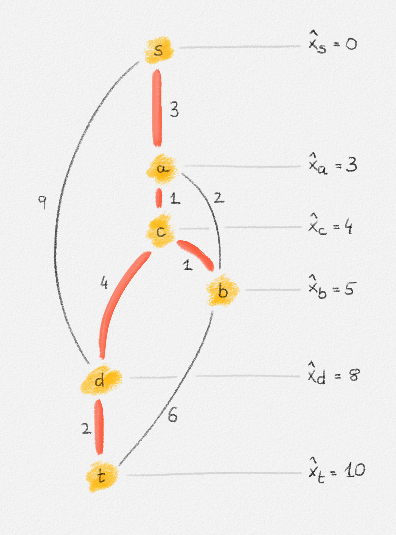
Figure 2.5: Illustration of the interpretation of (2.6) using the beads-and-string model. Holding the model from the vertex \(s\) makes each vertex hang the indicated distance below \(s\).

Thus, if \(\hat x_v\) represents how far below \(s\) we find \(v\), then gravity tries to maximize \(\sum_{v \in v} \hat x_v\). The condition that no string is being torn corresponds to the constraint that \(\hat x_v\) and \(\hat x_u\) can differ by at most \(w_{u,v}\), for every edge \((u,v)\) in the graph. Finally, once \(v\) has been pulled as far below \(s\) as possible by gravity, there must exist a path from \(s\) to \(v\) whose edges have been pulled tight. Otherwise, we would be able to pull \(v\) even farther away from \(s\). This path is a shortest path form \(s\) to \(v\), and its length is \(\hat x_v = \mathrm{dist}_{G,w}(s,v)\). The following lemma proves this claim formally.

Lemma 2.3: The optimal solution \(\hat x\) of the LP (2.6) satisfies \(\hat x_v = \mathrm{dist}_{G,w}(s,v)\) for all \(v \in V\).

Proof: Consider the subgraph \(H = (V,E') \subseteq G\) such that

\[E' = \bigl\{ (u,v) \in E \mid \hat x_v - \hat x_u = w_{u,v} \bigr\},\]

let \(S \subseteq V\) be the set of all vertices reachable from \(s\) in \(H\), and let \(T = V \setminus S\). See Figure 2.6.

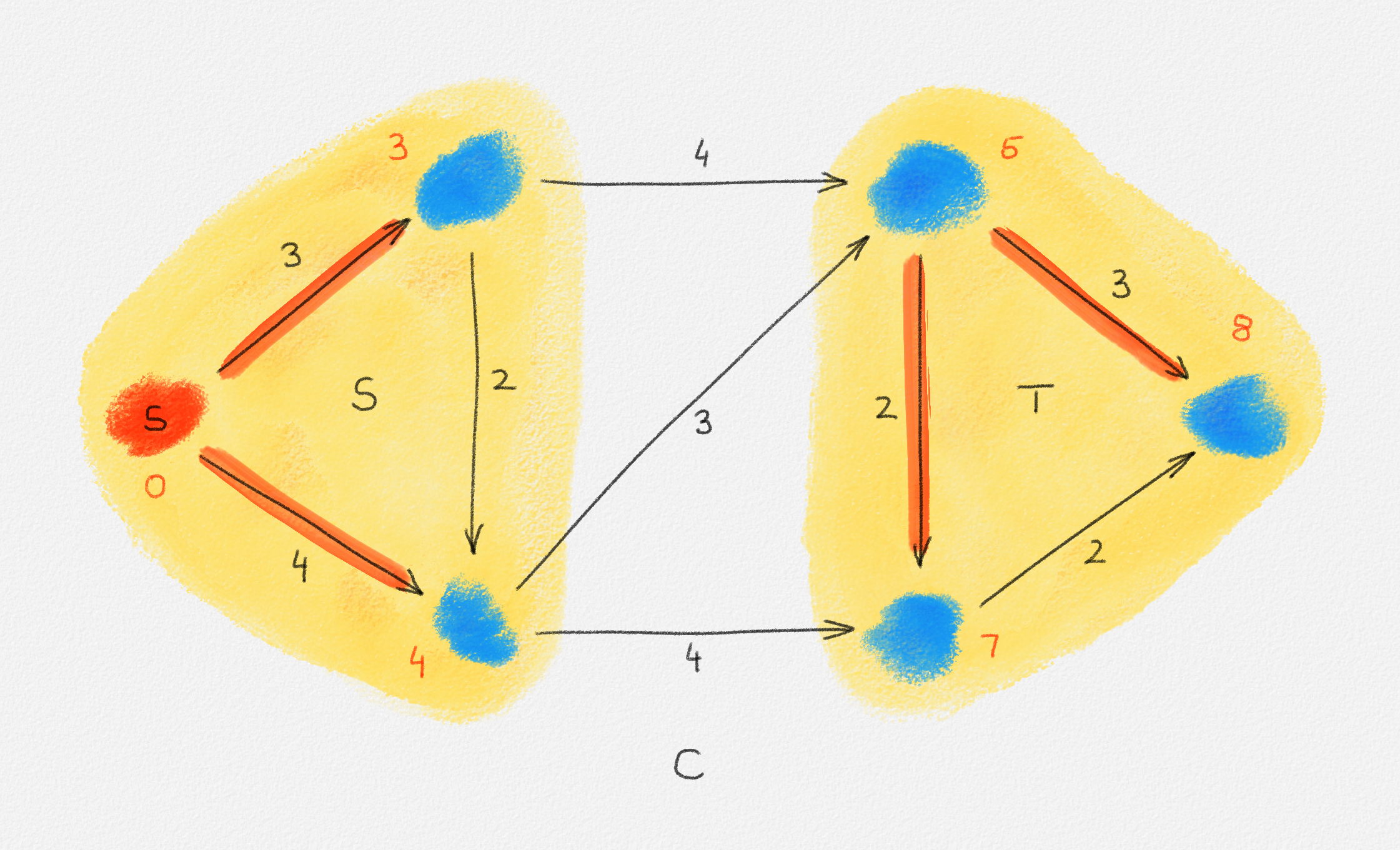
Figure 2.6: The sets \(S\) and \(T\) corresponding to the solution \(\hat x\) of (2.6) indicated by the red vertex labels. Black edge labels are the edge lengths. The red edges are tight and form the edge set of \(H\).

First we prove that \(T = \emptyset\), that is, that every vertex is reachable from \(s\) in \(H\).

Let

\[C = \{ (u,v) \in E \mid u \in S, v \in T \}.\]

Since every edge \((u,v) \in C\) has the property that \(u\) is reachable from \(s\) in \(H\) but \(v\) is not, it must satisfy \((u, v) \notin E'\) and, thus, \(\hat x_v - \hat x_u < w_{u,v}\). Therefore,

\[\delta = \min \bigl\{ w_{u,v} - \bigl(\hat x_v - \hat x_u\bigr) \mid (u,v) \in C \bigr\} > 0.\]

Now define a new solution \(\tilde x\) as

\[\tilde x_v = \begin{cases} \hat x_v & \text{if } v \in S\\ \hat x_v + \delta & \text{if } v \in T \end{cases}.\]

See Figure 2.7.

Figure 2.7: A solution \(\tilde x\) with a higher objective function value than the solution \(\hat x\) above. The new set \(S\) of vertices reachable from \(s\) is bigger.

Observe that \(s \in S\), so \(\tilde x_s = \hat x_s = 0\) because \(\hat x\) is a solution of (2.6).

For every edge \((u,v) \in E\), if \(v \in S\), then \(\tilde x_v = \hat x_v\) and \(\tilde x_u \ge \hat x_u\). Thus, \(\tilde x_v - \tilde x_u \le \hat x_v - \hat x_u \le w_{u,v}\).

If \(u, v \in T\), then \(\tilde x_v = \hat x_v + \delta\) and \(\tilde x_u = \hat x_u + \delta\). Thus, \(\tilde x_v - \tilde x_u = \hat x_v - \hat x_u \le w_{u, v}\).

Finally, if \(u \in S\) and \(v \in T\), then \(\tilde x_v = \hat x_v + \delta\) and \(\tilde x_u = \hat x_u\). Moreover, \((u, v) \in C\), so \(\delta \le w_{u, v} - \bigl(\hat x_v - \hat x_u\bigr)\). Therefore, \(\tilde x_v - \tilde x_u \le \hat x_v - \hat x_u + \delta \le w_{u,v}\).

This shows that \(\tilde x\) is a feasible solution of (2.6).

Next observe that \(\sum_{v \in V} \tilde x_v - \sum_{v \in V} \hat x_v = \delta|T|\). Since \(\tilde x\) is a feasible solution and \(\hat x\) is an optimal solution of (2.6), we have \(\sum_{v \in V} \tilde x_v - \sum_{v \in V} \hat x_v \le 0\), that is, \(T = \emptyset\) and \(S = V\).

The lemma now follows if every vertex \(v \in S\) satisfies \(\hat x_v = \mathrm{dist}_{G,w}(s,v)\). Let \(P = \langle v_0, \ldots, v_k \rangle\) be a path from \(s\) to \(v\) in \(H\). See Figure 2.8.

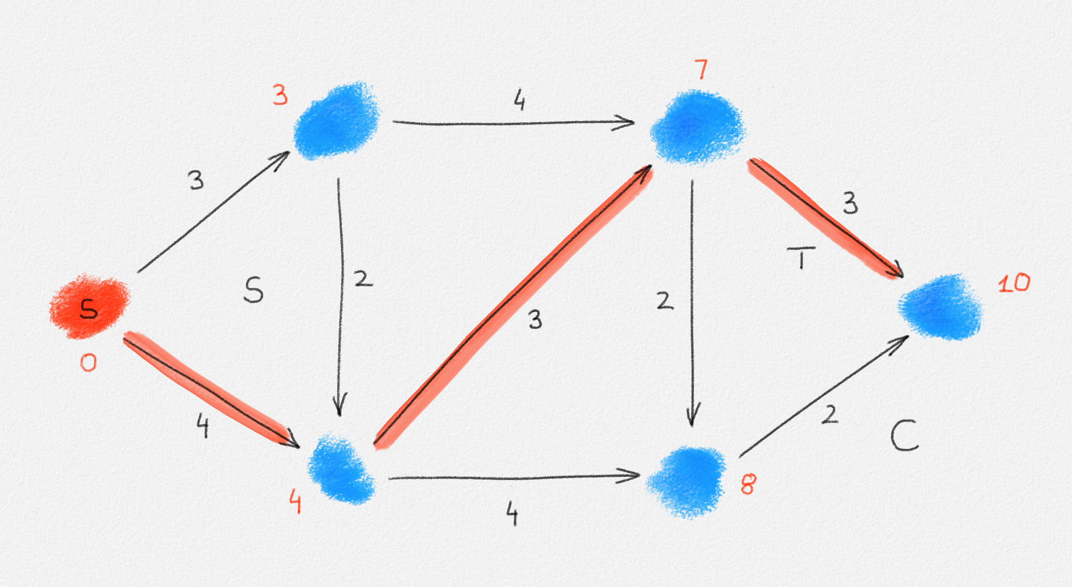
Figure 2.8: An optimal solution to (2.6) for the graph in Figure 2.6. The red path is a shortest path from \(s\) to the rightmost vertex.

Then \(\hat x_{v_0} = \hat x_s = 0\) and for \(1 \le i \le k\), \(\hat x_{v_i} = \hat x_{v_{i-1}} + w_{v_{i-1},v_i}\) because \(P\) is a path in \(H\). Thus,

\[\hat x_v = \hat x_{v_k} = \sum_{i=1}^k w_{v_{i-1},v_i} = w(P).\]

Since \(P\) is also a path from \(s\) to \(v\) in \(G \supseteq H\), this implies that

\[\hat x_v \ge \mathrm{dist}_{G,w}(s,v).\tag{2.7}\]

Conversely, for the shortest path \(\Pi_{G,w}(s,v) = \langle u_0, \ldots, u_\ell \rangle\) from \(s\) to \(v\) in \(G\), \(\hat x_{u_0} = \hat x_s = 0\) and, since \(\hat x\) is a solution of (2.6), \(\hat x_{u_i} \le \hat x_{u_{i-1}} + w_{u_{i-1},u_i}\) for all \(1 \le i \le \ell\). Thus,

\[\hat x_v = \hat x_{u_\ell} \le \sum_{i=1}^\ell w_{u_{i-1},u_i} = \mathrm{dist}_{G,w}(s,v).\tag{2.8}\]

Together, equations (2.7) and (2.8) show that \(\hat x_v = \mathrm{dist}_{G,w}(s,v)\). This finishes the proof. ▨

It may be useful to remind you at this point that our goal was to derive an LP formulation of the SSSP problem, that is, a linear program whose optimal solution consists of the distances from \(s\) to all vertices in \(G\). We proved that (2.6) is such an LP formulation. At this point, you may wonder how we go about finding such an optimal solution. We defer this discussion until Chapter 3, when we discuss the Simplex Algorithm. Our goal at this point is not to find optimal solutions to various optimization problems but to study how we can use linear programs as a mechanism to state these problems. We will later see that these formulations are useful because we can either solve the LPs using the Simplex Algorithm or the LP formulation sheds some light on the structure of the problem, which we can exploit in some algorithm we design to solve the problem.

2.3. Minimum Spanning Tree as an ILP

2.3.1. The Minimum Spanning Tree Problem

We have shown that the single-source shortest paths problem can be formulated as a linear program. Next let us look at a problem for which this is harder to do:

Given an edge-weighted connected undirected graph \((G,w)\), a minimum spanning tree (MST) of \((G,w)\) is a tree \(T = (V,E')\) with \(E' \subseteq E\) and such that every tree \(T' = (V,E'')\) with \(E'' \subseteq E\) satisfies \(w(E'') \ge w(E')\). See Figure 2.9.

Figure 2.9: A minimum spanning tree shown in red. The edge labels are the edge weights.

Minimum spanning tree problem: For an edge-weighted graph \((G,w)\), compute a spanning tree \(T\) of \(G\) of minimum weight.

2.3.2. Two Natural ILP Formulations of the MST Problem

The LP formulation of the SSSP problem is a fairly direct translation of the combinatorial formulation of the problem. When it comes to comparing greedy algorithms for the SSSP and MST problems, Kruskal's or Prim's algorithm seems to be more straightforward than Dijkstra's algorithm, at least in terms of the correctness proof. It is thus somewhat surprising that obtaining an efficient solution for the MST problem based on linear programming is significantly harder than for the SSSP problem.

Let us make a seemingly innocent change: We restrict the variables in the LP to being integers. An LP with this restriction is called, quite naturally, an integer linear program.

An integer linear program (ILP) is a linear program with the added constraint that all variable values in a feasible solution must be integers.

Since the MST problem is to choose the right subset of edges in \(E\) to be included in the edge set \(E'\) of the MST, it is natural to represent the set \(E'\) as a set of variables \(\{x_e \mid e \in E\}\) such that \(x_e = 1\) if \(e \in E'\) and \(x_e = 0\) if \(e \notin E'\). The weight of the MST \(T = (V, E')\) is then

\[w(T) = \sum_{e \in E} w_e x_e.\]

This is the objective function to be minimized. The constraints of the ILP need to enforce that \(T\) is a tree, that is, that \(T\) is connected and acyclic. The following exercise will be helpful in constructing the right set of constraints:

Exercise 2.3: Prove that a graph \(G\) on \(n\) vertices is a tree if and only if it has \(n - 1\) edges and

• Has no cycle or
• Is connected.

Our first two ILP formulations of the MST problem both enforce the constraint that \(T\) has \(n - 1\) edges:

\[\sum_{e \in E} x_e = n - 1.\]

To enforce that \(T\) is a tree, we need to add constraints that ensure that \(T\) is acyclic or that \(T\) is connected.

Enforcing That \(\boldsymbol{T}\) is Acyclic

Since \(T\) is a subgraph of \(G\), the only cycles that \(T\) can contain are cycles in \(G\). Thus, to ensure that \(T\) is acyclic, we need to ensure that there is no cycle \(C\) in \(G\) such that \(T\) contains all edges in \(C\); at least one edge from each cycle must be excluded from \(T\). This is easy to express as a set of linear constraints:

\[\sum_{e \in C} x_e \le |C| - 1 \quad \forall \text{cycle $C$ in $G$}.\]

This gives our first ILP formulation of the MST problem:

\[\begin{gathered} \text{Minimize } \sum_{e \in E} w_e x_e\\ \begin{aligned} \text{s.t. } \sum_{e \in E} x_e &= n - 1\\ \sum_{e \in C} x_e &\le |C| - 1 && \forall \text{cycle $C$ in $G$}\\ x_e &\in \{0, 1\} && \forall e \in E. \end{aligned} \end{gathered}\tag{2.9}\]

Note that this is an integer linear program: each variable \(x_e\) is not only constrained to be between \(0\) and \(1\)—this would make the problem a linear program—but is additionally required to be an integer. Since \(0\) and \(1\) are the only integers between \(0\) and \(1\), we thus require that \(x_e \in \{0, 1\}\) for all \(e \in E\).

Enforcing That \(\boldsymbol{T}\) is Connected

Our second ILP formulation of the MST problem ensures that \(T\) is a tree by requiring that it has \(n - 1\) edges and is connected. How can we express that a graph is connected? To do so, we need the notion of a cut:

A cut in a graph \(G = (V, E)\) is a partition of \(V\) into two non-empty subsets \(S\) and \(V \setminus S\). See Figure 2.10.

Figure 2.10: A cut \((S, V \setminus S)\). The red edges cross the cut.

Since the set \(V \setminus S\) is fixed once we specify \(S\), we will usually refer to any non-empty proper subset \(\emptyset \subset S \subset V\) as a cut. This ensures explicitly that \(S \ne \emptyset\), and the condition \(S \subset V\) ensures that \(V \setminus S \ne \emptyset\), so \((S, V \setminus S)\) is indeed the unique cut that has \(S\) as one of its halves.

An edge crosses the cut \(S\) if it has exactly one endpoint in \(S\). See Figure 2.10.

The following exercise shows how we can use cuts to express that a graph is connected.

Exercise 2.4: Prove that a graph \(G = (V,E)\) is connected if and only if every cut in \(G\) is crossed by at least one edge in \(E\).

Thus, our ILP formulation needs to ensure that the edge set \(E'\) of the tree \(T\) includes at least one edge that crosses each cut of \(G\):

\[\begin{gathered} \text{Minimize } \sum_{e \in E} w_e x_e\\ \begin{aligned} \text{s.t. } \sum_{e \in E} x_e &= n - 1\\ \sum_{e \text{ crosses } S} x_e &\ge 1 && \forall \text{cut $S$ in $G$}\\ x_e &\in \{0, 1\} && \forall e \in E. \end{aligned} \end{gathered}\tag{2.10}\]

From an algorithmic point of view, neither (2.9) nor (2.10) seems to be a very appealing formulation of the MST problem because they both involve a potentially exponential number of constraints: There can be an exponential number of cycles in \(G\) and there are \(2^{n-1} - 1\) cuts in an \(n\)-vertex graph. This suggests that solving either ILP should take exponential time. As we will see in Section 2.4, this is basically correct but not because the number of constraints is exponential but because integer linear programming is much harder than linear programming. So the "innocent change" to restrict variables to having integral values is far from innocent. In contrast, Prim's or Kruskal's algorithm can elegantly compute an MST in polynomial time.

2.3.3. An ILP Formulation of Polynomial Size*

In an attempt to reduce the difficulty of solving the MST problem formulated as an ILP, let us aim to develop an ILP formulation of the MST problem with only a polynomial number of constraints. The following, substantially less intuitive ILP formulation has only \(O\bigl(nm^2\bigr)\) constraints.

The tree structure of \(T\) is enforced using additional variables \(y_e^v \in \{0, 1\}\) and constraints on these variables. Fix an arbitrary vertex \(s \in V\). Then \(y_e^v = 1\) if and only if \(e\) belongs to the path from \(s\) to \(v\) in \(T\). Now the following observations capture that \(T\) is a tree:

• If the edge \((u,v)\) is in \(T\), then it belongs to the path from \(s\) to \(v\) or to the path from \(s\) to \(u\) but not both. If \((u,v) \notin T\), then it is not on any path. This can be expressed using the following constraint:

  \[y_{u,v}^u + y_{u,v}^v = x_{u,v} \quad \forall (u,v) \in E.\]

• Every vertex \(v \ne s\) has exactly one incident edge \((u,v)\) that belongs to the path from \(s\) to \(v\):

  \[\sum_{(u,v) \in E} y_{u,v}^v = 1 \quad \forall v \ne s.\]

  For \(v = s\), none of the edges incident to \(s\) belongs to the path from \(s\) to \(s\):

  \[\sum_{(s,v) \in E} y_{s,v}^s = 0.\]

• If the edge \((u,v)\) belongs to the path from \(s\) to \(v\) and the edge \((v,w)\) belongs to the path from \(s\) to some vertex \(z\), then the edge \((u,v)\) also belongs to the path from \(s\) to \(z\):

  \[y_{u,v}^z \ge y_{u,v}^v + y_{v,w}^z - 1 \quad \forall z \in V, (u,v) \in E, (v,w) \in E.\]

This gives the following ILP formulation of the MST problem:

\[\begin{gathered} \text{Minimize } \sum_{e \in E} w_e x_e\\ \begin{aligned} \text{s.t. } \phantom{y_{u,v}^u + y_{u,v}^v} \llap{\displaystyle\sum_{e \in E} x_e} &= n - 1\\ y_{u,v}^u + y_{u,v}^v &= x_{u,v} && \forall (u,v) \in E\\ \sum_{(s,v) \in E} y_{s,v}^s &= 0\\ \sum_{(u,v) \in E} y_{u,v}^v &= 1 && \forall v \ne s\\ y_{u,v}^z &\ge y_{u,v}^v + y_{v,w}^z - 1 && \forall z \in V, (u,v) \in E, (v,w) \in E\\ x_e &\in \{0, 1\} && \forall e \in E\\ y_e^v &\in \{0, 1\} && \forall v \in V, e \in E. \end{aligned} \end{gathered}\tag{2.11}\]

This ILP does indeed have polynomial size because, apart form the first three constraints, there are \(n - 1\) copies of the fourth constraint, one per vertex \(v \ne s\); no more than \(nm^2\) copies of the fifth constraint, at most one per vertex \(z \in V\) and per pair of edges \((u,v)\) and \((v, w)\) in \(E\); \(m\) copies of the sixth constraint, one per edge; and \(nm\) copies of the last constraint, one per pair \((v, e)\), where \(v\) is a vertex and \(e\) is an edge.

While the correctness of (2.9) and (2.10) should be obvious, the correctness of (2.11) requires some effort to prove. The next lemma and corollary show that it is indeed a correct formulation of the MST problem.

Lemma 2.4: For any undirected edge-weighted graph \((G,w)\), \(\bigl(\hat x, \hat y\bigr)\) is a feasible solution of (2.11) if and only if the subgraph \(T = (V, E')\) of \(G\) with \(E' = \bigl\{ e \in E \mid \hat x_e = 1 \bigr\}\) is a spanning tree of \(G\).

Proof: The first constraint of (2.11) ensures that every feasible solution \(\bigl(\hat x, \hat y\bigr)\) satisfies \(\sum_{e \in E} \hat x_e = n - 1\). Since an \(n\)-vertex graph is a tree if and only if it has \(n - 1\) edges and is acyclic, it therefore suffices to prove that \(\bigl(\hat x, \hat y\bigr)\) is a feasible solution of (2.11) if and only if \(T\) contains no cycle.

So assume first, for the sake of contradiction, that \(\bigl(\hat x, \hat y\bigr)\) is a feasible solution and that \(T\) contains a cycle \(C = \langle v_0, v_1, \ldots, v_k \rangle\). Then \(\hat x_{v_{i-1},v_i} = 1\) for all \(1 \le i \le k\). Since \(\hat y_{v_{i-1},v_i}^{v_{i-1}} + \hat y_{v_{i-1},v_i}^{v_i} = \hat x_{v_{i-1},v_i}\), this implies that either \(\hat y_{v_{i-1},v_i}^{v_{i-1}} = 1\) or \(\hat y_{v_{i-1},v_i}^{v_i} = 1\) for all \(1 \le i \le k\). If there exists a vertex \(v_i\) such that \(\hat y_{v_{i-1},v_i}^{v_i} = 1\) and \(\hat y_{v_i,v_{i+1}}^{v_i} = 1\), then \(\sum_{(u,v_i) \in E} \hat y_{u,v_i}^{v_i} > 1\), a contradiction. Thus, we can assume w.l.o.g. that \(\hat y_{v_{i-1},v_i}^{v_i} = 1\) and \(\hat y_{v_{i-1},v_i}^{v_{i-1}} = 0\) for all \(1 \le i \le k\). In particular, \(y_{v_0,v_1}^{v_0} = 0\).

Now observe that \(\hat y_{v_{i-1},v_i}^{v_k} = 1\) for all \(1 \le i \le k\). The proof is by induction on \(j = k - i\). For the base case, \(i = k\), we just observed that \(\hat y_{v_{k-1},v_k}^{v_k} = 1\). For the inductive step, \(i < k\), observe that, by the inductive hypothesis, \(\hat y_{v_i,v_{i+1}}^{v_k} = 1\). Since \(\hat y_{v_{i-1},v_i}^{v_i} = 1\), \(\hat y_{v_{i-1},v_i}^{v_k} \ge \hat y_{v_{i-1},v_i}^{v_i} + y_{v_i,v_{i+1}}^{v_k} - 1\), and \(\hat y_{v_{i-1},v_i}^{v_k} \in \{0,1\}\), we have \(\hat y_{v_{i-1},v_i}^{v_k} = 1\).

Since \(\hat y_{v_{i-1},v_i}^{v_k} = 1\) for all \(1 \le i \le k\), we have in particular that \(\hat y_{v_0,v_1}^{v_k} = 1\). Since \(C\) is a cycle, we have \(v_k = v_0\), that is, \(\hat y_{v_0,v_1}^{v_0} = 1\), a contradiction because we observed above that \(\hat y_{v_0, v_1}^{v_0} = 0\). Thus, \(T\) cannot contain any cycles if \(\bigl(\hat x, \hat y\bigr)\) is a feasible solution of (2.11).

Now assume that \(T\) is a tree and define \(\hat x_e = 1\) if and only if \(e \in T\) and \(\hat y_e^v = 1\) if and only if the edge \(e\) is on the path from \(s\) to \(v\) in \(T\). Since \(T\) has \(n - 1\) edges, we have \(\sum_{e \in E} \hat x_e = n - 1\).

If we consider an edge \((u, v) \in T\), then let \(T_u\) and \(T_v\) be the two subtrees of \(T\) obtained by removing the edge \((u, v)\). See Figure 2.11.

Figure 2.11: The two subtrees \(T_u\) and \(T_v\) of \(T\) obtained by removing the edge \((u, v)\).

If \(s \in T_u\), then \((u, v)\) belongs to the path from \(s\) to \(v\) but not to the path from \(s\) to \(u\). If \(s \in T_v\), then \((u, v)\) belongs to the path from \(s\) to \(u\) but not to the path from \(s\) to \(v\). In both cases, \(\hat y_{u,v}^u + \hat y_{u,v}^v = 1 = \hat x_{u,v}\). If \((u, v) \notin T\), then \(\hat y_{u,v}^u + \hat y_{u,v}^v = 0 = \hat x_{u,v}\).

Since no edge in \(T\) belongs to the path from \(s\) to \(s\), we have \(\sum_{(s, v) \in E} \hat y_{s,v}^s = 0\). For \(v \ne s\), let \(u_1, \ldots, u_d\) be the neighbours of \(v\) in \(T\). Removing the edges \((u_1,v), \ldots, (u_d,v)\) breaks \(T\) into \(d + 1\) connected components. One contains only \(v\); the others are subtrees \(T_{u_1}, \ldots, T_{u_d}\) containing the vertices \(u_1, \ldots, u_d\), respectively. There exists exactly one such tree \(T_{u_i}\) that contains \(s\). In this case, the edge \((u_i,v)\) belongs to the path from \(s\) to \(v\) and the other edges \((u_j,v)\) with \(j \ne i\) do not. Thus, \(\sum_{j=1}^d \hat y_{u_j,v}^v = \sum_{(u,v) \in E} \hat y_{u,v}^v = 1\). See Figure 2.12.

Figure 2.12: Exactly one of the edges incident to a vertex \(v \ne s\) belongs to the path from \(s\) to \(v\).

Finally, consider any two edges \((u,v), (v,w) \in E\) sharing an endpoint and any vertex \(z \in V\). If \((u,v)\) does not belong to the path from \(s\) to \(v\), then \(\hat y_{u,v}^v = 0\). If \((v,w)\) does not belong to the path from \(s\) to \(z\), then \(\hat y_{v,w}^z = 0\). In either case, \(\hat y_{u,v}^v + \hat y_{v,w}^z - 1 \le 0\). Thus, \(\hat y_{u,v}^z \ge 0 \ge \hat y_{u,v}^v + \hat y_{v,w}^z - 1\).

If \((u,v)\) belongs to the path from \(s\) to \(v\), and \((u,v)\) and \((v,w)\) belong to the path from \(s\) to \(z\), then \(\hat y_{u,v}^v = \hat y_{v,w}^z = 1\) and \(\hat y_{u,v}^z = 1 = \hat y_{u,v}^v + \hat y_{v,w}^z - 1\).

If \((u,v)\) belongs to the path from \(s\) to \(v\), \((v,w)\) belongs to the path from \(s\) to \(z\), and \((u,v)\) does not belong to the path from \(s\) to \(z\), then let \(P_1\) be the path from \(s\) to \(v\) in \(T\), and let \(P_2\) be the path from \(s\) to \(z\) in \(T\). Since the edge \((v,w)\) belongs to \(P_2\), so does the vertex \(v\). The subpath \(P_2'\) of \(P_2\) from \(s\) to \(v\) does not contain \((u,v)\) because \(P_2\) does not contain \((u,v)\). Thus, \(T\) contains two paths from \(s\) to \(v\), a contradiction because \(T\) is a tree. Therefore, this is not possible. In other words, \(\hat y_{u,v}^v = 1\) and \(\hat y_{v,w}^z = 1\) implies that \(\hat y_{u,v}^z = 1 = \hat y_{u,v}^v + \hat y_{v,w}^z - 1\). See Figure 2.13.

Figure 2.13: If \((u, v)\) belongs to the path from \(s\) to \(v\) and \((v, w)\) belongs to the path from \(s\) to \(z\) but \((u, v)\) does not, then \(T\) cannot be a tree.

This shows that the solution \(\bigl(\hat x, \hat y\bigr)\) corresponding to \(T\) is a feasible solution of (2.11). ▨

Since every feasible solution \(\bigl(\hat x, \hat y\bigr)\) of (2.11) defines a spanning tree of \(G\) and vice versa, we have:

Corollary 2.5: For any undirected edge-weighted graph \((G,w)\), \(\bigl(\hat x, \hat y\bigr)\) is an optimal solution of (2.11) if and only if the subgraph \(T = (V, E')\) of \(G\) with \(E' = \bigl\{ e \in E \mid \hat x_e = 1 \bigr\}\) is an MST of \((G,w)\).

The ILP (2.11) has only a polynomial number of constraints, while (2.9) and (2.10) have an exponential number of constraints. As we discuss next, this does not make (2.11) any easier to solve. The key to an efficient solution of the minimum spanning tree problem is to express it as a linear program, without requiring that the variables have integer values. It turns out that this is much easier to do for a slightly modified version of (2.9) than for any of the three ILPs (2.9), (2.10), and (2.11).

2.4. The Computational Complexity of LP and ILP

Now that we know what linear programs and integer linear programs are, and we got a glimpse of how to model optimization problems as LPs or ILPs, the next question is how we find optimal solutions for LPs and ILPs.

Linear Programming

In Chapter 3, we discuss the Simplex Algorithm as a classical algorithm for solving LPs. The Simplex Algorithm is the most popular algorithm for solving linear programs in practice, and it is also among the fastest algorithms in practice to solve many LPs. For some pathological inputs, however, the Simplex Algorithm may take exponential time and thus does not find a solution efficiently. Remarkably, any such pathological input has an almost identical input "nearby" that takes the Simplex Algorithm polynomial time to solve (Spielman and Teng, 2004). Thus, we have to try really, really hard if we want to make the Simplex Algorithm take exponential time.

Still, in theory, the Simplex Algorithm is not a polynomial-time algorithm. The Ellipsoid Algorithm and Karmarkar's Algorithm, not discussed here, can solve every linear program in polynomial time. More importantly, the Ellipsoid Algorithm can do that even for LPs with an exponential number of constraints, provided these constraints are represented appropriately: The Ellipsoid Algorithm relies on a "separation oracle" to drive its search for an optimal solution. Even if the LP technically has an exponential number of constraints, it may be possible to implement a separation oracle for the LP that runs in polynomial time and space. If that's the case, then the Ellipsoid Algorithm solves the LP in polynomial time. In practice, the Ellipsoid Algorithm suffers from numerical instability and is much slower than both the Simplex Algorithm and Karmarkar's Algorithm.

Even though we do not discuss the Ellipsoid Algorithm or Karmarkar's algorithm in these notes, the main take-away from this short subsection is that

Theorem 2.6: Any linear program can be solved in polynomial time in its size.

Integer Linear Programming

So we can solve linear programs in polynomial time. What about integer linear programs? In the remainder of this section, we prove that solving integer linear programs is NP-hard, even if they have only a polynomial number of constraints.

Recall the basic strategy for proving that a problem \(\Pi\) is NP-hard. It suffices to provide a polynomial-time reduction from an NP-hard problem \(\Pi'\) to \(\Pi\). Specifically, we need to provide a polynomial-time algorithm \(\mathcal{A}\) that takes any instance \(I'\) of \(\Pi'\) and computes from it an instance \(I\) of \(\Pi\) such that \(I\) is a yes-instance of \(\Pi\) if and only if \(I'\) is a yes-instance of \(\Pi'\). If you have not seen any NP-hardness proofs yet or you need a refresher on how they work, the appendix provides a brief introduction to the topic.

Here, we choose \(\Pi\) to be ILP and \(\Pi'\) to be the satisfiability problem (SAT). A SAT instance is a Boolean formula in CNF over some set of variables \(x_1, \ldots, x_n\):

\[\begin{aligned} F &= C_1 \wedge \cdots \wedge C_m\\ C_i &= \lambda_{i1} \vee \cdots \vee \lambda_{ik_i} && \forall 1 \le i \le m\\ \lambda_{ij} &\in \{ x_1, \ldots, x_n, \bar x_1, \ldots, \bar x_n \} && \forall 1 \le i \le m, 1 \le j \le k_i. \end{aligned}\]

\(\bar x_i\) denotes the negation of \(x_i\).

We translate \(F\) into an ILP over variables \(x_1, \ldots, x_n \in \{0,1\}\). Each literal \(\lambda_{ij}\) is translated into a linear function \(\phi_{ij}(x_1, \ldots, x_n)\) defined as

\[\phi_{ij}(x_1, \ldots, x_n) = \begin{cases} x_k & \text{if } \lambda_{ij} = x_k\\ 1 - x_k & \text{if } \lambda_{ij} = \bar x_k \end{cases}.\]

Each clause \(C_i\) is translated into the constraint

\[\Phi_i(x_1, \ldots, x_n) \ge 1,\]

where

\[\Phi_i(x_1, \ldots, x_n) = \sum_{j=1}^{k_i} \phi_{ij}(x_1, \ldots, x_n).\]

It turns out that even deciding whether this ILP has a feasible solution is NP-hard, so we can choose any objective function, such as \(f(x_1, \ldots, x_n) = 0\), to complete the definition of the ILP.

To prove that deciding whether this ILP has a feasible solution is NP-hard, we prove that \(F\) is satisfiable if and only if the ILP has a feasible solution:

First assume that \(F\) is satisfiable. Then there exists an assignment \(\hat x = \bigl(\hat x_1, \ldots, \hat x_n\bigr)\) of truth values to the variables \(x_1, \ldots, x_n\) in \(F\) such that every clause \(C_i\) contains a true literal \(\lambda_{ij}\). For this literal, \(\phi_{ij}\bigl(\hat x_1, \ldots, \hat x_n\bigr) = 1\). Thus, since \(\phi_{ij'}\bigl(\hat x_1, \ldots, \hat x_n\bigr) \ge 0\) for all \(1 \le j' \le k_i\), \(\Phi_i\bigl(\hat x_1, \ldots, \hat x_n\bigr) = \sum_{j'=1}^{k_i} \phi_{ij'}\bigl(\hat x_1, \ldots, \hat x_n\bigr) \ge 1\), that is, \(\hat x\) satisfies the constraint corresponding to \(C_i\) in the ILP. Since \(\hat x\) satisfies every clause of \(F\), this shows that it satisfies every constraint of the ILP, so \(\hat x\) is a feasible solution of the ILP.

Now assume that the ILP is feasible. Then there exists a feasible solution \(\hat x = \bigl(\hat x_1, \ldots, \hat x_n\bigr)\) of the ILP. Since \(\hat x_i \in \{0, 1\}\) for all \(1 \le i \le n\), we can interpret this solution as an assignment of truth values to the variables \(x_1, \ldots, x_n\) in \(F\). Since \(\hat x\) is a feasible solution of the ILP, we have \(\Phi_i\bigl(\hat x_1, \ldots, \hat x_n\bigr) = \sum_{j'=1}^{k_i} \phi_{ij'}\bigl(\hat x_1, \ldots, \hat x_n\bigr) \ge 1\) for every clause \(C_i\). Thus, \(\phi_{ij}\bigl(\hat x_1, \ldots, \hat x_n\bigr) = 1\) for at least one literal \(\lambda_{ij} \in C_i\), that is, \(\lambda_{ij}\) is made true by the solution \(\hat x = \bigl(\hat x_1, \ldots, \hat x_n\bigr)\) and, thus, \(C_i\) is satisfied by \(\hat x\). Since \(\hat x\) satisfies every constraint in the ILP, it also satisfies every clause \(C_i\) in \(F\), that is, it is a satisfying truth assignment of \(F\).

We have shown that we can, in polynomial time, convert any Boolean formula \(F\) into an ILP that is feasible if and only if \(F\) is satisfiable. This conversion is a polynomial-time reduction from SAT to ILP. Since SAT is NP-hard, this proves that

Theorem 2.7: Integer linear programming is NP-hard.

2.5. LP Relaxations

Given that we have polynomial-time algorithms for solving LPs but solving ILPs is NP-hard, an important question is whether we can use the machinery for solving LPs to obtain suboptimal but good solutions for ILPs. We will explore this question in the third part of this book. Here, we introduce an important tool for translating ILPs into related LPs: LP relaxation.

For every ILP, one can define a corresponding LP by simply dropping the requirement that the solution value of each variable be an integer: in the LP solution, variables are allowed to take on any real values as long as they satisfy the constraints in the LP.

The LP relaxation of an ILP is the same as the ILP, but the requirement that the variable values in a feasible solution be integers is dropped.

As an example, here is the LP relaxation of (2.9). It is identical to the ILP, except that the constraint \(x_e \in \{0, 1\}\) has been replaced with the constraint \(0 \le x_e \le 1\): \(x_e\) is no longer required to be integral:

\[\begin{gathered} \text{Minimize } \sum_{e \in E} w_e x_e\\ \begin{aligned} \text{s.t. } \sum_{e \in E} x_e &= n - 1\\ \sum_{e \in C} x_e &\le |C| - 1 && \forall \text{cycle $C$ in $G$}\\ 0 &\le x_e \le 1 && \forall e \in E. \end{aligned} \end{gathered}\tag{2.12}\]

In general, the LP relaxation of an ILP may have a much better optimal solution than the ILP itself, but it can never have a worse optimal solution:

Lemma 2.8: If \(\hat x\) is an optimal solution to a minimization ILP \(P\) and \(\tilde x\) is an optimal solution to its LP relaxation \(P'\), then \(f\bigl(\tilde x\bigr) \le f\bigl(\hat x\bigr)\), where \(f\) is the objective function shared by \(P\) and \(P'\).

Proof: Since \(\hat x\) is a feasible solution of \(P\), it is also a feasible solution of \(P'\). Since \(\tilde x\) is an optimal solution of \(P'\), this implies that \(f\bigl(\tilde x\bigr) \le f\bigl(\hat x\bigr)\). ▨

The ratio \(f\bigl(\hat x\bigr) \mathop{/} f\bigl(\tilde x\bigr)\) between the optimal objective function values of the ILP and its relaxation is called the integrality gap of the ILP.

In general, this gap can be arbitrarily large. However, for problems where the integrality gap is bounded, the LP relaxation can often be used to efficiently obtain an approximation of the optimal solution of the ILP, a fact that will be explored further when we discuss Chapter 13. Another useful property exploited by some approximation algorithms is half-integrality of the optimal solution of some LPs: In the optimal solution, every variable takes on a value that is a multiple of \(\frac{1}{2}\). Again, this will be explored further when discussing approximation algorithms.

2.5.1. ILPs With Integrality Gap 1

In some instances, the optimal solution of the LP relaxation of an ILP is integral, that is, every variable has an integer value. By Lemma 2.8, this implies that the optimal solution of the LP relaxation is also an optimal solution of the ILP.

In the remainder of this section, we explore whether the MST problem is such a problem. The answer depends on the chosen ILP formulation. For each of (2.9), (2.10), and (2.11), there exists an input that has a fractional solution with a lower objective function value than the best possible integral solution, as shown in the following three examples.

The "No Cycles" Formulation

As already observed, the LP relaxation of (2.9) is

\[\begin{gathered} \text{Minimize } \sum_{e \in E} w_e x_e\\ \begin{aligned} \text{s.t. } \sum_{e \in E} x_e &= n - 1\\ \sum_{e \in C} x_e &\le |C| - 1 && \forall \text{cycle $C$ in $G$}\\ 0 &\le x_e \le 1 && \forall e \in E. \end{aligned} \end{gathered}\tag{2.13}\]

Any MST of the graph in Figure 2.14 has weight \(10\).

Figure 2.14: The edge labels are edge weights. The red tree has weight \(10\) and is an MST.

On the other hand, the following fractional solution with objective function value \(6\) satisfies all constraints of (2.13):¹

\[\begin{aligned} x_{12} &= 0\\ x_{23} = x_{24} = x_{25} = x_{26} &= \frac{1}{2}\\ x_{37} = x_{47} = x_{57} = x_{67} &= 1 \end{aligned}\]

The "Connectivity" Formulation

The LP relaxation of (2.10) is

\[\begin{gathered} \text{Minimize } \sum_{e \in E} w_e x_e\\ \begin{aligned} \text{s.t. } \sum_{e \in E} x_e &= n - 1\\ \sum_{e \text{ crosses } S} x_e &\ge 1 && \forall \text{cut $S$ in $G$}\\ 0 &\le x_e \le 1 && \forall e \in E. \end{aligned} \end{gathered}\tag{2.14}\]

Any MST of the graph in Figure 2.15 has weight \(2\).

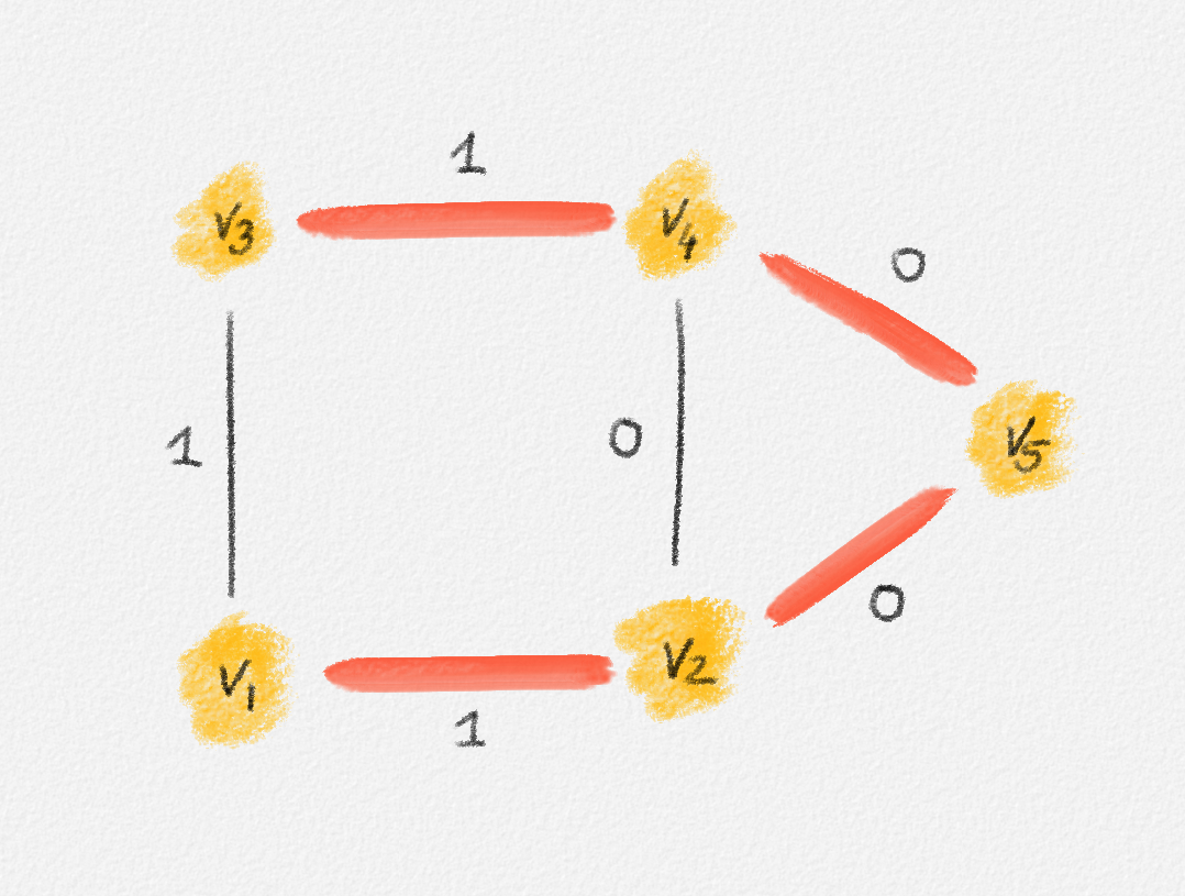
Figure 2.15: The edge labels are edge weights. The red tree has weight \(2\) and is an MST.

On the other hand, the following fractional solution with objective function value \(\frac{3}{2}\) satisfies all constraints of (2.12):

\[\begin{aligned} x_{12} = x_{13} = x_{24} = x_{34} &= \frac{1}{2}\\ x_{25} = x_{45} &= 1 \end{aligned}\]

The Polynomial-Size Formulation

The LP relaxation of (2.11) is

\[\begin{gathered} \text{Minimize } \sum_{e \in E} w_e x_e\\ \begin{aligned} \text{s.t. } \phantom{y_{(u,v)}^u + y_{(u,v)}^v} \llap{\displaystyle\sum_{e \in E} x_e} &= n - 1\\ y_{u,v}^u + y_{u,v}^v &= x_{u,v} && \forall (u,v) \in E\\ \sum_{(s,v) \in E} y_{s,v}^s &= 0\\ \sum_{(u,v) \in E} y_{u,v}^v &= 1 && \forall v \ne s\\ y_{u,v}^z &\ge y_{u,v}^v + y_{v,w}^z - 1\quad && \forall z \in V, (u,v) \in E, (v,w) \in E\\ 0 \le x_e &\le 1 && \forall e \in E\\ 0 \le y_e^v &\le 1 && \forall v \in V, e \in E. \end{aligned} \end{gathered}\tag{2.15}\]

Any MST of the graph in Figure 2.16 has weight \(10\).

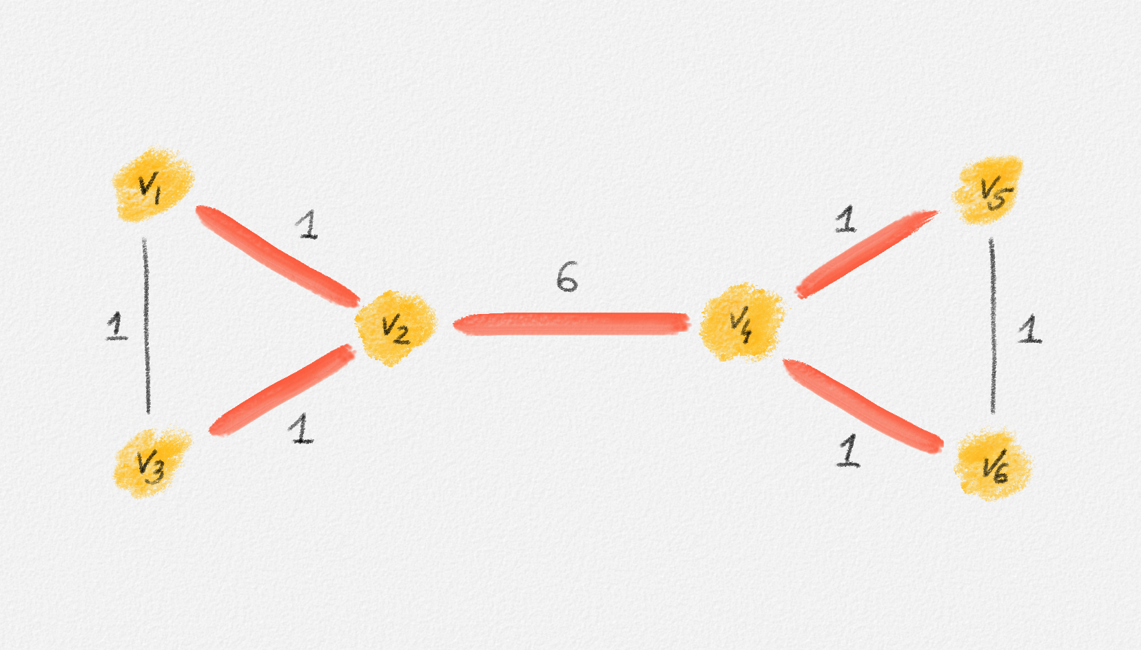
Figure 2.16: The edge labels are edge weights. The red tree has weight \(10\) and is an MST.

No matter whether \(s = v_1\) or \(s = v_2\) (any other choice is symmetric to one of these two choices), there exists a feasible solution of (2.15) whose objective function value is only \(5\):

\[\begin{aligned} \boldsymbol{s = v_1:} && x_{13} = x_{24} &= 0 & x_{12} &= x_{23} = x_{45} = x_{46} = x_{56} = 1\\ && y_{13}^k = y_{24}^k &= 0 \quad \forall 1 \le k \le 6 & y_{45}^k &= y_{46}^k = y_{56}^k = \frac{1}{2} \quad \forall 1 \le k \le 6\\ && y_{12}^k &= 0 \quad \forall k \notin \{2, 3\} & y_{12}^k &= 1 \quad \forall k \in \{2, 3\}\\ && y_{23}^k &= 0 \quad \forall k \ne 3 & y_{23}^3 &= 1 \end{aligned}\]

\[\begin{aligned} \boldsymbol{s = v_2:} && x_{13} = x_{24} &= 0 & x_{12} &= x_{23} = x_{45} = x_{46} = x_{56} = 1\\ && y_{13}^k = y_{24}^k &= 0\quad \forall 1 \le k \le 6 & y_{45}^k &= y_{46}^k = y_{56}^k = \frac{1}{2} \quad \forall 1 \le k \le 6\\ && y_{12}^k &= 0 \quad \forall k \ne 1 & y_{12}^1 &= 1\\ && y_{23}^k &= 0 \quad \forall k \ne 3 & y_{23}^3 &= 1 \end{aligned}\]

As these three examples show, integrality matters for all three MST ILPs (2.9), (2.10), and (2.11). Next, we discuss an extension of (2.9) whose LP relaxation has an optimal integral solution.

2.5.2. An ILP Formulation of the MST Problem With Integrality Gap 1

The following extension of (2.9) finally is an ILP whose LP relaxation has an optimal integral solution:

\[\begin{gathered} \text{Minimize } \sum_{e \in E} w_e x_e\\ \begin{aligned} \text{s.t. } \phantom{\displaystyle\sum_{\substack{(u,v) \in E\\u,v \in S}} x_{u,v}} \llap{\displaystyle\sum_{e \in E} x_e} &\ge n - 1\\ \sum_{\substack{(u,v) \in E\\u,v \in S}} x_{u,v} &\le |S| - 1 && \forall \emptyset \subset S \subseteq V\\ x_e &\in \{0, 1\} && \forall e \in E. \end{aligned} \end{gathered}\tag{2.16}\]

This is an extension of (2.9) because it does not only require that at most \(k - 1\) edges of every \(k\)-vertex cycle in \(G\) are chosen as part of the spanning tree but that at most \(k - 1\) edges between any subset of \(k\) vertices are chosen. Given that not including any cycle in \(T\) is what makes \(T\) a tree, it is surprising that this seemingly unimportant strengthening of the ILP ensures that the LP relaxation has an integral optimal solution. Let's first establish the correctness of the ILP.

Lemma 2.9: For any undirected edge-weighted graph \((G, w)\), \(\hat x\) is a feasible solution of (2.14) if and only if the subgraph \(T = (V, E')\) of \(G\) with \(E' = \bigl\{e \in E \mid \hat x_e = 1\bigr\}\) is a spanning tree of \(G\).

Proof: First note that the constraints \(\sum_{(u,v) \in E; u,v \in S} x_{u,v} \le |S| - 1\) ensure exactly that \(T\) is a forest, that is, \(T\) contains no cycles: If \(T\) contains a cycle \(C\) with vertex set \(S_C \ne \emptyset\), then \(\sum_{(u,v) \in E; u,v \in S_C} \hat x_{u,v} \ge |S_C|\), violating the constraint \(\sum_{(u,v) \in E; u,v \in S_C} x_{u,v} \le |S_C| - 1\).

Conversely, if \(T\) contains no cycle, then the subgraph

\[T[S] = (S, \{ (u,v) \in E' \mid u,v \in S \})\]

is a forest for every subset \(\emptyset \subset S \subseteq V\). Thus,

\[|\{ (u,v) \in E' \mid u,v \in S \}| = \sum_{(u,v) \in E; u,v \in S} \hat x_{u,v} \le |S| - 1,\]

that is, \(\hat x\) satisfies the constraint

\[\sum_{(u,v) \in E; u,v \in S} x_{u,v} \le |S| - 1\]

for every subset \(\emptyset \subset S \subseteq V\).

Finally, observe that the constraints

\[\sum_{e \in E} x_e \ge n - 1\]

and

\[\sum_{(u,v) \in E; u,v \in S} x_{(u,v)} \le |S| - 1\]

for \(S = V\) imply that

\[\sum_{e \in E} x_e = n - 1,\]

that is, \(|E'| = n - 1\).

Thus, \(\hat x\) satisfies the constraints in (2.16) if and only if \(T\) is a forest with \(n - 1\) edges, which is a tree. ▨

Once again, this one-to-one correspondence between feasible solutions of the ILP and spanning trees implies that

Corollary 2.10: For any undirected edge-weighted graph \((G, w)\), \(\hat x\) is an optimal solution of (2.16) if and only if the subgraph \(T = (V, E')\) of \(G\) with \(E' = \bigl\{e \in E \mid \hat x_e = 1\bigr\}\) is an MST of \((G, w)\).

As the following example shows, if there are edges of equal weight in \((G, w)\), then the LP relaxation of (2.16) may once again have an optimal fractional solution:

Consider the graph in Figure 2.17. The corresponding LP relaxation of (2.16) is

\[\begin{gathered} \text{Minimize } 3x_{12} + 2x_{13} + x_{24} + 3x_{34}\\ \begin{aligned} \text{s.t. } x_{12} + x_{13} + x_{24} + x_{34} &\ge 3\\ x_{12} + x_{13} + x_{24} + x_{34} &\le 3\\ x_{12} + x_{13} &\le 2\\ x_{12} + x_{24} &\le 2\\ x_{13} + x_{34} &\le 2\\ x_{24} + x_{34} &\le 2\\ 0 \le x_e &\le 1 \quad \forall e \in E, \end{aligned} \end{gathered}\tag{2.17}\]

which has the optimal fractional solution

\[x_{12} = \alpha \qquad x_{34} = 1 - \alpha \qquad x_{13} = x_{24} = 1,\]

for any \(0 \le \alpha \le 1\).

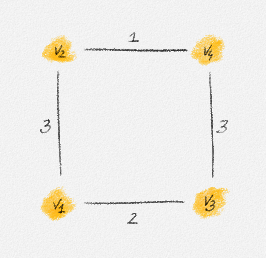
Figure 2.17: Since the edges \((v_1, v_2)\) and \((v_3, v_4)\) have the same weight, any fractional solution of (2.17) with \(x_{12} = \alpha\), \(x_{34} = 1 - \alpha\), and \(x_{13} = x_{24} = 1\) is an optimal solution.

It is easily verified that, at least in this example, any optimal fractional solution has the same objective function value as an optimal integral solution, that is, the optimal solution of the ILP is also an optimal solution of its relaxation. As we will show in Section 4.4, this is always the case. (We postpone the proof because we do not have the tools to construct the proof yet.) Moreover, it can be shown that if we use the Simplex Algorithm to find a solution of the LP relaxation of (2.16), the computed solution is always integral. The proof uses two facts that we do not prove here:

• Recall that the feasible region of an LP is a convex polytope in \(\mathbb{R}^n\). A geometric view of the Simplex Algorithm is that it moves between vertices of this polytope until it reaches a vertex that represents an optimal solution.

• Every vertex of the polytope defined by the LP relaxation of (2.16) represents an integral solution.

How useful is it that the LP relaxation of (2.16) has an integral optimal solution, given that this LP has exponentially many constraints? Doesn't it still take exponential time to solve this LP even using an algorithm whose running time is polynomial in the number of constraints? As mentioned in Section 2.4, the Ellipsoid Algorithm can solve every LP in polynomial time for which we can provide a polynomial-time separation oracle. The constraints in the LP relaxation of (2.16) are derived from the given edge-weighted graph \((G,w)\), whose representation uses only polynomial space, and it turns out that an appropriate separation oracle for the MST problem can be implemented in polynomial time based on this graph representation, without explicitly inspecting all constraints. Thus, the LP relaxation of (2.16) can in fact be solved in polynomial time. Still, sticking to Kruskal's or Prim's algorithm seems to be the much easier and generally more efficient approach for computing MSTs. The purpose of the Section 2.3 and of this section was simply to illustrate linear programming using a more elaborate example and to introduce integer linear programming and LP relaxations.

2.6. Canonical Form and Standard Form

So far, we have focused on discussing how to model some optimization problems using LPs. More examples will follow in subsequent chapters: Linear programming will be used as a tool to express optimization problems throughout this book. Chapter 3 is concerned with discussing the most widely used algorithm for solving LPs, the Simplex Algorithm. This algorithm assumes that its input is in a particular form. This section introduces two standard representations of linear programs, the canonical form and the standard form; the latter, sometimes also called slack form, is the one the Simplex Algorithm works with.¹ Canonical form is important as the basis for the theory of LP duality, which will be the basis for a number of algorithms discussed in these notes.

2.6.1. Canonical Form

An LP over a set of variables \(x_1, \ldots, x_n\) is in canonical form if

• It is a maximization LP,

• Every variable \(x_i\) is required to be non-negative: The LP contains a non-negativity constraint

  \[x_i \ge 0\]

  for every variable \(x_i\).

• All other constraints are upper bound constraints: They provide a constant upper bound on some linear combination of the variables. For example:

  \[x_1 + 3x_2 - 2x_4 \le 20.\]

We can represent such an LP as an \(n\)-element row vector

\[c = (c_1, \ldots, c_n),\]

an \(m\)-element column vector

\[b = \begin{pmatrix} b_1\\ b_2\\ \vdots\\ b_m \end{pmatrix},\]

and an \(m \times n\) matrix

\[A = \begin{pmatrix} a_{1,1} & a_{1,2} & \cdots & a_{1,n}\\ a_{2,1} & a_{2,2} & \cdots & a_{2,n}\\ \vdots & \vdots & \ddots & \vdots\\ a_{m,1} & a_{m,2} & \cdots & a_{m,n} \end{pmatrix}.\]

\(A\), \(b\), and \(c\) represent the following LP in canonical form:

\[\begin{gathered} \text{Maximize } \sum_{j=1}^n c_jx_j\\ \begin{aligned} \text{s.t. }\sum_{j=1}^n a_{ij}x_j &\le b_i && \forall 1 \le i \le m && \text{(upper bound constraints)}\\ x_j &\ge 0 && \forall 1 \le j \le n && \text{(non-negativity constraints)} \end{aligned} \end{gathered}\]

If we define that \(x \le y\) for two \(m\)-element vectors if and only if \(x_i \le y_i\) for all \(1 \le i \le m\), and we write \(0\) to denote the \(0\)-vector \((0, \ldots, 0)^T\),¹ then this LP can be written more compactly as

\[\begin{gathered} \text{Maximize } cx\\ \begin{aligned} \text{s.t. } Ax &\le b\\ x &\ge 0, \end{aligned} \end{gathered}\tag{2.18}\]

where \(cx\) is the inner product of the two vectors \(c\) and \(x\) and \(Ax\) is the usual matrix-vector product. (Throughout the remainder of this chapter and throughout the next two chapters, we treat \(x\) as a column vector.)

Throughout most of these notes, we adopt the following definition of equivalence of two LPs:

Two LPs are equivalent if

• They have the same variables,
• They have the same set of feasible solutions, and
• Their objective functions assign the same value to each feasible solution.

In the following two lemmas, we use a more general notion of equivalence of LPs, which considers two LPs \(P\) and \(P'\) over variables \(x = (x_1, \ldots, x_n)^T\) and \(y = (y_1, \ldots, y_r)^T\) equivalent if there exist two linear functions \(\phi : \mathbb{R}^n \rightarrow \mathbb{R}^r\) and \(\psi : \mathbb{R}^r \rightarrow \mathbb{R}^n\) such that

• \(\hat x\) is a feasible solution of \(P\) if and only if \(\phi\bigl(\hat x\bigr)\) is a feasible solution of \(P'\),
• \(\hat y\) is a feasible solution of \(P'\) if and only if \(\psi\bigl(\hat y\bigr)\) is a feasible solution of \(P\),
• If \(\hat x\) is an optimal solution of \(P\), then \(\phi\bigl(\hat x\bigr)\) is an optimal solution of \(P'\), and
• If \(\hat y\) is an optimal solution of \(P'\), then \(\psi\bigl(\hat y\bigr)\) is an optimal solution of \(P\).

Less formally, this says that \(\phi\) and \(\psi\) are mappings between solutions of \(P\) and \(P'\) that preserve feasible solutions and optimal solutions.

Equivalence of LPs is useful because it allows us to obtain an optimal solution of an LP by solving any of its equivalent LPs. By the following lemma, every LP has an equivalent LP in canonical form:

Lemma 2.11: Every linear program can be transformed into an equivalent linear program in canonical form.

Proof: An LP \(P\) may not be in canonical form for four reasons:

• It may be a minimization LP.
• Some of its constraints may be equality constraints.
• Some of its inequality constraints may be lower bounds, as opposed to upper bounds.
• Some variables may not have non-negativity constraints.

We define a sequence of LPs \(P = P_0, P_1, P_2, P_3, P_4 = P'\) such that \(P'\) is in canonical form and for all \(1 \le i \le 4\), \(P_{i-1}\) and \(P_i\) are equivalent. Thus, \(P'\) is an LP in canonical form that is equivalent to \(P\).

From minimization LP to maximization LP: First we construct a maximization LP \(P_1\) that is equivalent to \(P_0 = P\). If \(P_0\) is itself a maximization LP, then \(P_1 = P_0\). Otherwise, the objective of \(P_0\) is to minimize \(cx\). This is the same as maximizing \(-cx\). Thus, \(P_1\) has the objective function \(-cx\) and asks us to maximize it. \(P_0\) and \(P_1\) have the same variables and the same constraints, so they have the same set of feasible solutions. As just observed, any feasible solution that minimizes \(cx\) also maximizes \(-cx\). Thus, \(P_0\) and \(P_1\) are equivalent.

From equalities to inequalities: The next LP \(P_2\) we construct from \(P_1\) is a maximization LP without equality constraints. Clearly,

\[\sum_{j=1}^n a_{ij}x_j = b_i\]

if and only if

\[\begin{aligned} \sum_{j=1}^n a_{ij}x_j &\ge b_i \text{ and}\\ \sum_{j=1}^n a_{ij}x_j &\le b_i. \end{aligned}\]

Thus, we construct \(P_2\) by replacing every equality constraint in \(P_1\) with these two corresponding inequality constraints. \(P_1\) and \(P_2\) have the same variables and the same objective function, and every inequality constraint in \(P_1\) is also a constraint in \(P_2\). As just observed, any solution \(\hat x = \bigl(\hat x_1, \ldots, \hat x_n\bigr)\) satisfies an equality constraint in \(P_1\) if and only if it satisfies the two corresponding inequality constraints in \(P_2\). Thus, \(P_1\) and \(P_2\) have the same set of feasible solutions and the same objective function. They are therefore equivalent.

From lower bounds to upper bounds: The next LP \(P_3\) we construct from \(P_2\) is a maximization LP with only upper bound constraints. This transformation is similar to the transformation from a minimization LP to a maximization LP: Every lower bound constraint

\[\sum_{j=1}^n a_{ij}x_j \ge b_i\]

in \(P_2\) is satisfied if and only if the upper bound constraint

\[\sum_{j=1}^n -a_{ij}x_j \le -b_i\]

is satisfied, so we replace it with this constraint in \(P_3\). Since \(P_2\) and \(P_3\) have the same variables and the same objective function, and it is easy to see that \(\hat x = \bigl(\hat x_1, \ldots, \hat x_n\bigr)\) is a feasible solution of \(P_2\) if and only if it is a feasible solution of \(P_3\), \(P_2\) and \(P_3\) are equivalent.

Introducing non-negativity constraints: \(P_3\) is in canonical form, except that it does not include non-negativity constraints for its variables. To obtain the final LP \(P_4 = P'\) in canonical form, we replace every variable in \(P_3\) with a pair of non-negative variables in \(P_4\).

\(P_4\) has the set of variables

\[\bigl\{x_j', x_j'' \mid 1 \le j \le n\bigr\}.\]

The objective function and constraints of \(P_4\) are obtained from the objective function and constraints of \(P_3\) by replacing every occurrence of \(x_j\) with \(x_j' - x_j''\) for all \(1 \le j \le n\) and by adding non-negativity constraints for all variables of \(P_4\). The resulting LP \(P_4\) is in canonical form.

The linear transformations \(\phi\) and \(\psi\) that establish the equivalence between \(P_3\) and \(P_4\) are defined as follows:

\[\phi(x_1, \ldots, x_n) = \bigl(x_1', x_1'', \ldots, x_n', x_n''\bigr),\]

where

\[\begin{aligned} x_j' &= \begin{cases} x_j & \text{if } x_j \ge 0\\ 0 & \text{if } x_j < 0 \end{cases}\\ x_j'' &= \begin{cases} 0 & \text{if } x_j \ge 0\\ -x_j & \text{if } x_j < 0 \end{cases} \end{aligned}\]

for all \(1 \le j \le n\), and

\[\psi\bigl(x_1', x_1'', \ldots, x_n', x_n''\bigr) = (x_1, \ldots, x_n),\]

where

\[x_j = x_j' - x_j''\]

for all \(1 \le j \le n\).

Given a feasible solution \(\bigl(\hat x_1, \ldots, \hat x_n\bigr)\) of \(P_3\), let \(\bigl(\hat x_1', \hat x_1'', \ldots, \hat x_n', \hat x_n''\bigr) = \phi\bigl(\hat x_1, \ldots, \hat x_n\bigr)\). By the definition of \(\phi\), all values \(\hat x_1', \hat x_1'', \ldots, \hat x_n', \hat x_n''\) are non-negative. Moreover, we have \(\hat x_j' - \hat x_j'' = \hat x_j\) for all \(1 \le j \le n\). Since \(\bigl(\hat x_1, \ldots, \hat x_n\bigr)\) satisfies all constraints of \(P_3\) and every occurrence of \(x_j\) in \(P_3\) is replaced with \(x_j' - x_j''\) in \(P_4\), for all \(1 \le j \le n\), \(\bigl(\hat x_1', \hat x_1'', \ldots, \hat x_n', \hat x_n''\bigr)\) satisfies all constraints of \(P_4\) and achieves the same objective function value as \(\bigl(\hat x_1, \ldots, \hat x_n\bigr)\).

Conversely, given a feasible solution \(\bigl(\hat x_1', \hat x_1'', \ldots, \hat x_n', \hat x_n''\bigr)\) of \(P_4\), let \(\bigl(\hat x_1, \ldots, \hat x_n\bigr) = \psi\bigl(\hat x_1', \hat x_1'', \ldots, \hat x_n', \hat x_n''\bigr)\). Then, once again, \(\hat x_j' - \hat x_j'' = \hat x_j\) for all \(1 \le j \le n\). Since \(\bigl(\hat x_1', \hat x_1'', \ldots, \hat x_n', \hat x_n''\bigr)\) satisfies all constraints of \(P_4\) and every occurrence of \(x_j\) in \(P_3\) is replaced with \(x_j' - x_j''\) in \(P_4\), for all \(1 \le j \le n\), \(\bigl(\hat x_1, \ldots, \hat x_n\bigr)\) satisfies all constraints of \(P_3\) and achieves the same objective function value as \(\bigl(\hat x_1', x_1'', \ldots, \hat x_n', x_n''\bigr)\).

Since \(\phi\) and \(\psi\) map feasible solutions to feasible solutions and preserve their objective function values, it follows that \(\phi\bigl(x_1, \ldots, x_n)\) is an optimal solution of \(P_4\) if \(\bigl(x_1, \ldots, x_n\bigr)\) is an optimal solution of \(P_3\), and \(\psi\bigl(x_1', x_1'', \ldots, x_n', x_n''\bigr)\) is an optimal solution of \(P_3\) if \(\bigl(x_1', x_1'', \ldots, x_n', x_n''\bigr)\) is an optimal solution of \(P_4\). Thus, \(P_3\) and \(P_4\) are equivalent. ▨

Here is an illustration of the transformation in the proof of Lemma 2.11. It uses a slightly modified version of an LP used later when discussing minimum-cost flows in Chapter 6. This LP describes a flow through a graph \(G\) whose edges are partitioned into two subsets \(E_b\) and \(E_u\). The LP has one variable \(p_v\) per vertex \(v \in V\) and one variable \(s_{u,v}\) for every edge \((u, v) \in E_b\). There is no variable corresponding to any edge in \(E_u\). The values \(q_{u,v}\) are constants:

\[\begin{gathered} \text{Minimize } \sum_{(u,v) \in E_b} c_{u,v}s_{u,v} - \sum_{u \in V} b_up_u\\ \begin{aligned} \text{s.t. } p_u - p_v - s_{u,v} &\le q_{u,v} && \forall (u,v) \in E_b\\ p_v - p_u &\ge q_{u,v} && \forall (u,v) \in E_u\\ s_{u,v} &\ge 0 && \forall (u,v) \in E_b \end{aligned} \end{gathered}\]

I will first illustrate the process outlined in the above proof verbatim, without modifications. Then I will discuss some shortcuts one may take to arrive at the result faster, and at a simpler result.

First we turn the LP into a maximization LP:

\[\text{Maximize } \sum_{u \in V} b_up_u - \sum_{(u,v) \in E_b} c_{u,v}s_{u,v}\]

There are no equality constraints, so the second transformation is not needed. Next, we turn lower bounds into upper bounds:

\[\begin{aligned} p_u - p_v - s_{u,v} &\le q_{u,v} && \forall (u,v) \in E_b\\ p_u - p_v &\le -q_{u,v} && \forall (u,v) \in E_u\\ -s_{u,v} &\le 0 && \forall (u,v) \in E_b \end{aligned}\]

Finally, we replace every variable \(p_v\) with the difference \(p'_v - p''_v\) of two non-negative variables \(p'_v\) and \(p''_v\), and we do the same for variables \(s_{u,v}\). This gives the following LP in canonical form:

\[\begin{gathered} \text{Maximize } \sum_{u \in V} b_up_u' - \sum_{u \in V} b_up_u'' - \sum_{(u,v) \in E_b} c_{u,v}s_{u,v}' + \sum_{(u,v) \in E_b} c_{u,v}s_{u,v}''\\ \begin{aligned} \text{s.t. } p_u' - p_u'' - p_v' + p_v'' - s_{u,v}' + s_{u,v}'' &\le q_{u,v} && \forall (u,v) \in E_b\\ p_u' - p_u'' - p_v' + p_v'' &\le -q_{u,v} && \forall (u,v) \in E_u\\ s_{u,v}'' - s_{u,v}' &\le 0 && \forall (u,v) \in E_b\\ p_v' &\ge 0 && \forall v \in V\\ p_v'' &\ge 0 && \forall v \in V\\ s_{u,v}' &\ge 0 && \forall (u,v) \in E_b\\ s_{u,v}'' &\ge 0 && \forall (u,v) \in E_b \end{aligned} \end{gathered}\]

While reading through this example, I hope that you thought that it was silly to turn the constraint \(s_{u,v} \ge 0\) into the constraint \(-s_{u,v} \le 0\) as part of the elimination of lower bound constraints, only to then split \(s_{u,v}\) into two non-negative variables \(s'_{u,v}\) and \(s''_{u,v}\). This is the primary shortcut we take in practice:

We leave any lower bound constraint of the form \(x_i \ge 0\) alone during the conversion of lower bound constraints into upper bound constraints, because it is simply a non-negativity constraint. Any variable for which the input LP has such a non-negativity constraint can be included unaltered in the output LP, exactly because it is already constrained to be non-negative: We do not need to split it. In our example, this means that we leave the variables \(s_{u,v}\) and their non-negativity constraints alone and only split each variable \(p_v\) into the two variables \(p'_v\) and \(p''_v\):

\[\begin{gathered} \text{Maximize } \sum_{u \in V} b_up_u' - \sum_{u \in V} b_up_u'' - \sum_{(u,v) \in E_b} c_{u,v}s_{u,v}\\ \begin{aligned} \text{s.t. } p_u' - p_u'' - p_v' + p_v'' - s_{u,v} &\le q_{u,v} && \forall (u,v) \in E_b\\ p_u' - p_u'' - p_v' + p_v'' &\le -q_{u,v} && \forall (u,v) \in E_u\\ p_v' &\ge 0 && \forall v \in V\\ p_v'' &\ge 0 && \forall v \in V\\ s_{u,v} &\ge 0 && \forall (u,v) \in E_b \end{aligned} \end{gathered}\]

A similar simplification concerns variables that are constrained to be non-positive in the input LP: \(x_i \le 0\). Instead of keeping this upper bound constraint and then replacing \(x_i\) with \(x_i' - x_i''\), where \(x_i' \ge 0\) and \(x_i'' \ge 0\), we observe that \(x_i \le 0\) is really a non-negativity constraint on \(-x_i\). Thus, we can simply replace every occurrence of \(x_i\) in the input LP with \(-x_i'\) and then convert the resulting constraint \(-x_i' \le 0\) into the non-negativity constraint \(x_i' \ge 0\).

To summarize:

• Any unconstrained variable \(x_i\) is replaced by the difference \(x_i' - x_i''\) of two non-negative variables \(x_i'\) and \(x_i''\).

• Any variable with a non-negativity constraint in the input LP is included without change in the output LP, as is its non-negativity constraint.

• Any variable \(x_i\) with a non-positivity constraint in the input LP is replaced with \(-x_i'\), and its non-positivity constraint \(x_i \le 0\) is replaced with a non-negativity constraint \(x_i' \ge 0\).

This reduces the number of variables in the output LP because we introduce two variables in the output LP only for unconstrained variables in the input LP.

2.6.2. Standard Form

The Simplex Algorithm expects its input in standard form.

An LP is in standard form if it has \(m + n\) variables \(x_1, \ldots, x_n, y_1, \ldots, y_m\) and is of the form:¹

\[\begin{gathered} \text{Maximize } \sum_{j=1}^n c_jx_j + d\\ \begin{aligned} \text{s.t. } y_i &= b_i - \sum_{j=1}^n a_{ij} x_j && \forall 1 \le i \le m\\ x_j &\ge 0 && \forall 1 \le j \le n\\ y_i &\ge 0 && \forall 1 \le i \le m \end{aligned} \end{gathered}\]

The variables \(y_1, \ldots, y_m\) are called basic variables (sometimes also slack variables). The variables \(x_1, \ldots, x_n\) are called non-basic variables.

Note that

• Only non-basic variables appear in the objective function. An alternative view, which we will take later is that all basic variables appear in the objective function with coefficient \(0\).

• There is a one-to-one correspondence between the equality constraints in the LP and the basic variables: The \(i\)th basic variable \(y_i\) occurs only in the \(i\)th equality constraint, with coefficient \(1\). Again, another way to say this is that the \(i\)th basic variable \(y_i\) has coefficient \(1\) in the \(i\)th equality constraint and coefficient \(0\) everywhere else.

If we collect the basic variables \(y_1, \ldots, y_m\) in a column vector \(y = (y_1, \ldots, y_m)^T\), the constant terms \(b_1, \ldots, b_m\) in a column vector \(b = (b_1, \ldots, b_m)^T\), the non-basic variables \(x_1, \ldots, x_n\) in a column vector \(x = (x_1, \ldots, x_n)^T\), the objective function coefficients \(c_1, \ldots, c_n\) in a row vector \(c = (c_1, \ldots, c_n)\), and the coefficients \(a_{ij}\) in a matrix \(A\), then we obtain a compact formulation of standard form similar to the compact formulation of canonical form (2.18):

\[\begin{gathered} \text{Maximize } cx + d\\ \begin{aligned} \text{s.t. } y &= b - Ax\\ x &\ge 0\\ y &\ge 0, \end{aligned} \end{gathered}\tag{2.19}\]

Once again, \(0\) is used to denote appropriate column vectors all of whose components are \(0\).

Since we want to use the Simplex Algorithm to solve arbitrary LPs but the Simplex Algorithm expects its input in standard form, we need to answer the question whether we can convert any LP into an equivalent one in standard form. Lemma 2.11 shows that we can convert any LP into an equivalent one in canonical form. The next lemma shows that any such LP in canonical form can be converted into an equivalent one in standard form. By chaining these two transformations together, we obtain a transformation of an arbitrary LP into an equivalent one in standard form.

Lemma 2.12: Every linear program in canonical form can be transformed into an equivalent linear program in standard form.

Proof: Consider the following two LPs:

\[\begin{gathered} \text{Maximize } \sum_{j=1}^n c_jx_j\\ \begin{aligned} \text{s.t. } \sum_{j=1}^n a_{ij} x_j &\le b_i && \forall 1 \le i \le m\\ x_j &\ge 0 && \forall 1 \le j \le n \end{aligned} \end{gathered}\tag{2.20}\]

\[\begin{gathered} \text{Maximize } \sum_{j=1}^n c_jx_j\\ \begin{aligned} \text{s.t. } y_i &= b_i - \sum_{j=1}^n a_{ij} x_j && \forall 1 \le i \le m\\ x_j &\ge 0 && \forall 1 \le j \le n\\ y_i &\ge 0 && \forall 1 \le i \le m \end{aligned} \end{gathered}\tag{2.21}\]

(2.20) is in canonical form. (2.21) is in standard form. We claim that they are equivalent.

Any feasible solution \(\hat x = \bigl(\hat x_1, \ldots, \hat x_n\bigr)\) of (2.20) can be extended to a feasible solution \(\bigl(\hat x, \hat y\bigr)\) of (2.21) by setting \(\hat y_i = b_i - \sum_{j=1}^n a_{ij}\hat x_j\) for all \(1 \le i \le m\). This explicitly ensures that \(\bigl(\hat x, \hat y\bigr)\) satisfies all equality constraints of (2.21). It also ensures that \(\hat x_j \ge 0\) for all \(1 \le j \le n\) and \(\hat y_i \ge 0\) for all \(1 \le i \le m\) because \(\hat x\) is a feasible solution of (2.20) and, therefore, \(\sum_{j=1}^n a_{ij}\hat x_j \le b_i\). Thus, \(\bigl(\hat x, \hat y\bigr)\) is a feasible solution of (2.21). Its objective function value in (2.21) is the same as the objective function value of \(\hat x\) in (2.20), because (2.20) and (2.21) have the same objective function.

Now consider any feasible solution \(\bigl(\hat x, \hat y\bigr)\) of (2.21). Then \(\hat x\) is a feasible solution of (2.20): Indeed, we have \(\hat x_j \ge 0\) for all \(1 \le j \le n\) because \(\bigl(\hat x, \hat y\bigr)\) is a feasible solution of (2.21). We also have \(\hat y_i = b_i - \sum_{j=1}^n a_{ij}x_j\) and \(\hat y_i \ge 0\) for all \(1 \le i \le m\). Thus, \(\sum_{j=1}^n a_{ij}x_j \le b_i\) for all \(1 \le i \le m\). Once again, since (2.20) and (2.21) have the same objective function, \(\bigl(\hat x, \hat y\bigr)\) and \(\hat x\) achieve the same objective function values as solutions of (2.21) and (2.20), respectively.

Since every feasible solution of (2.20) has a corresponding feasible solution of (2.21) with the same objective function value and vice versa, it follows that the feasible solution of (2.21) associated with an optimal solution of (2.20) is an optimal solution of (2.17) and vice versa. Thus, (2.20) and (2.21) are equivalent. ▨

In Section 2.6.1, we gave an example of converting an arbitrary LP into an equivalent one in canonical form. Next we continue this example by converting the LP in canonical form into an equivalent one in standard form. The LP in canonical form we obtained was

\[\begin{gathered} \text{Maximize } \sum_{u \in V} b_up_u' - \sum_{u \in V} b_up_u'' - \sum_{(u,v) \in E_b} c_{u,v}s_{u,v}\\ \begin{aligned} \text{s.t. } p_u' - p_u'' - p_v' + p_v'' - s_{u,v} &\le q_{u,v} && \forall (u,v) \in E_b\\ p_u' - p_u'' - p_v' + p_v'' &\le -q_{u,v} && \forall (u,v) \in E_u\\ p_v' &\ge 0 && \forall v \in V\\ p_v'' &\ge 0 && \forall v \in V\\ s_{u,v} &\ge 0 && \forall (u,v) \in E_b. \end{aligned} \end{gathered}\tag{2.22}\]

To convert this LP into standard form, we introduce a slack variable \(y_{u,v}\) for every edge \((u, v) \in E\) and rewrite the upper bound constraints in (2.22) as equality constraints:

\[\begin{gathered} \text{Maximize } \sum_{u \in V} b_up_u' - \sum_{u \in V} b_up_u'' - \sum_{(u,v) \in E_b} c_{u,v}s_{u,v}\\ \begin{aligned} \text{s.t. } y_{u,v} &= q_{u,v} - p_u' + p_u'' + p_v' - p_v'' + s_{u,v} && \forall (u,v) \in E_b\\ y_{u,v} &= -q_{u,v} - p_u' + p_u'' + p_v' - p_v'' && \forall (u,v) \in E_u\\ p_v' &\ge 0 && \forall v \in V\\ p_v'' &\ge 0 && \forall v \in V\\ s_{u,v} &\ge 0 && \forall (u,v) \in E_b\\ y_{u,v} &\ge 0 && \forall (u,v) \in E \end{aligned} \end{gathered}\]

The following alternative representation of standard form will be more useful for manipulating LPs in the Simplex Algorithm and in many other circumstances. We can clearly write (2.19) as

\[\begin{gathered} \text{Maximize } cx + d\\ \begin{aligned} \text{s.t. } b &= y + Ax\\ x &\ge 0\\ y &\ge 0, \end{aligned} \end{gathered}\]

which is the same as

\[\begin{gathered} \text{Maximize } 0y + cx + d\\ \begin{aligned} \text{s.t. } b &= Iy + Ax\\ x &\ge 0\\ y &\ge 0, \end{aligned} \end{gathered}\tag{2.23}\]

where \(I\) is the \(m \times m\) identity matrix and \(0\) is the \(m\)-element \(0\)-vector.

Now let \(c'\) be the concatenation of \(0\) and \(c\), \[c' = (\underbrace{0, \ldots, 0}_{m\ \text{times}}, c_1, \ldots, c_n),\]

let

\[A' = [I|A] = \left( \begin{matrix} 1 & 0 & \cdots & 0\\ 0 & 1 & \cdots & 0\\ \vdots & \vdots & \ddots & \vdots\\ 0 & 0 & \cdots & 1\\ \end{matrix} \,\left|\, \begin{matrix} a_{1,1} & a_{1,2} & \cdots & a_{1,n}\\ a_{2,1} & a_{2,2} & \cdots & a_{2,n}\\ \vdots & \vdots & \ddots & \vdots\\ a_{m,1} & a_{m,2} & \cdots & a_{m,n} \end{matrix} \right. \right),\]

and let

\[z = \begin{pmatrix} z_1\\ \vdots\\ z_{m+n} \end{pmatrix} = \begin{pmatrix} y_1\\ \vdots\\ y_m\\ x_1\\ \vdots\\ x_n \end{pmatrix}.\]

Then (2.23) becomes

\[\begin{gathered} \text{Maximize } c'z + d\\ \begin{aligned} \text{s.t. } b &= A'z\\ z &\ge 0. \end{aligned} \end{gathered}\tag{2.24}\]

An LP written in this form is in standard form if it is equipped with a basis \(B = \{ j_1, \ldots, j_m \} \subseteq \{ 1, \ldots, m + n \}\)² of \(m\) indices such that for all \(1 \le i \le m\), \(c_{j_i} = 0\), \(a_{ij_i} = 1\), and \(a_{ij} = 0\) for all \(1 \le j \le m\) with \(j \ne j_i\). The variables \(z_{j_1}, \ldots, z_{j_m}\) are the basic variables of the LP. To clearly associate each index \(j_i \in B\) with the \(i\)th equality constraint in (2.24), we write \(B\) as a vector \((j_1, \ldots, j_m)\), not as a set, but we still use standard set notation such as \(h \in B\) to indicate that an index \(h\) occurs in this vector. The above translation of (2.23) into (2.24) together with the basis \(B = (1, \ldots, m)\) clearly satisfies these conditions.

3. The Simplex Algorithm

In this chapter, we discuss the Simplex Algorithm, a classical and fairly simple algorithm for solving linear programs, that is, for finding optimal solutions of linear programs. As discussed in Section 2.4, the Simplex Algorithm does not run in polynomial time in the worst case, but it is remarkably fast in practice.

The Simplex Algorithm expects its input in standard form. By Lemmas 2.11 and 2.12, every LP can be transformed into an equivalent LP in standard form. Thus, this is not a restriction. Throughout this chapter, all LPs will be in standard form, so we simply refer to them as linear programs without explicitly stating the assumption that they are in standard form.

The Simplex Algorithm can be summarized as follows: Every LP in standard form has a unique special solution called its basic solution. If this solution is feasible, it is called a basic feasible solution (BFS¹). The first step of the Simplex Algorithm is to decide whether the given LP \(P\) is feasible, whether it has a feasible solution at all. If it doesn't, the algorithm terminates and reports that \(P\) is infeasible. If \(P\) has a feasible solution, then the Simplex Algorithm transforms it into an equivalent LP \(P^{(0)}\) whose basic solution is feasible. Recall the concept of equivalence of two LPs: They have the same set of feasible solutions and assign the same objective function value to any such solution. Thus, the BFS of \(P^{(0)}\) is also a feasible solution of \(P\). After constructing \(P^{(0)}\), the Simplex Algorithm continues to transform this LP, producing a sequence of LPs \(P^{(0)}, \ldots, P^{(t)}\) that are all equivalent to \(P\) and all have basic feasible solutions. The transformation of each LP \(P^{(s)}\) into the next LP \(P^{(s+1)}\), called pivoting, also ensures that the BFS of \(P^{(s+1)}\) has an objective function value that is no less, ideally greater, than the objective function value of the BFS of \(P^{(s)}\). Thus, the algorithm makes steady progress towards better and better solutions. Once the Simplex Algorithm can verify that the BFS of the current LP \(P^{(t)}\) is optimal, something that is particularly easy to check for a BFS, it terminates and reports this solution. Since \(P^{(t)}\) is equivalent to \(P\), this solution must also be an optimal solution of \(P\).

This chapter is organized as follows:

• In Section 3.1, we introduce the concepts of the basic solution and of the basic feasible solution (BFS) of an LP.

• Section 3.2 gives an overview of the Simplex Algorithm.

• Section 3.3 discusses pivoting, the basic operation used by the Simplex Algorithm to move from BFS to BFS in search of an optimal solution.

• This discussion assumes that the basic solution of the initial LP is feasible. In general, this may not be the case. Thus, we need to discuss how to test whether the initial LP has any feasible solution and, if so, how to transform it into an equivalent LP whose basic solution is feasible. Section 3.4 discusses how to do this. Remarkably, we use the Simplex Algorithm itself, applying it to an auxiliary LP, to perform this step—how's that for bootstrapping!

• The previous four sections amount to a complete description of the Simplex Algorithm. Section 3.5 rounds out this discussion using an extended example and, in the process, introduces a tabular representation of an LP, called a tableau. Pivoting is easy to implement on a tableau using elementary row operations. Thus, tableaux are essential for the efficient implementation of the Simplex Algorithm and may also aid your intuition about how the Simplex Algorithm works. I encourage you to peek ahead at this section while reading the earlier sections of this chapter to connect the formal discussion of the Simplex Algorithm to the mechanics of performing the different steps on a concrete example.

• The final section, Section 3.6, considers cycling, a problem that can cause the Simplex Algorithm to run forever. The pivoting step gives us a lot of freedom in how we transform a given LP \(P^{(s)}\) into the next LP \(P^{(s+1)}\). If we are not careful, then some sequence of pivoting steps may transform a given LP back into itself. That's cycling: The algorithm cycles through the same set of LPs forever. We discuss Bland's rule, one of many rules that specify the details of the pivoting step in a way that prevents cycling. As part of the discussion of cycling and of Bland's rule as a means to avoid cycling, we provide an (exponential) upper bound on the running time of the Simplex Algorithm. We defer the correctness proof of the algorithm until we discuss LP duality in Chapter 4 because we need LP duality to complete the proof.

3.1. Basic Solutions and Basic Feasible Solutions

A vector \(\hat z\) is called a basic solution of the LP \(P\)

\[\begin{gathered} \text{Maximize } cz + d\\ \begin{aligned} \text{s.t. } b &= Az\\ z &\ge 0 \end{aligned} \end{gathered}\]

with basis \(B = (j_1, \ldots, j_m)\) if \(b = A\hat z\) and \(\hat z_j = 0\) for all \(j \notin B\). In other words, only basic variables can be non-zero in a basic solution.

Since the LP is in standard form, we have \(c_j = 0\) for all \(j \in B\), so the requirement that \(\hat z_j = 0\) for all \(j \notin B\) implies that the objective function value of a basic solution is \(c\hat z + d = d\).

Since \(a_{ij_i} = 1\) and \(a_{ij} = 0\) for all \(j \in B \setminus \{j_i\}\), we also have

\[b_i = \hat z_{j_i} + \sum_{j \notin B} a_{ij}\hat z_{j} = \hat z_{j_i}\]

for all \(1 \le i \le m\). Thus,

Every LP has exactly one basic solution \(\hat z\) defined as

\[\hat z_j = \begin{cases} b_i & \text{if } j = j_i \in B\\ 0 & \text{if } j \notin B, \end{cases}\]

and we call it the basic solution of the LP.

Since \(\hat z_{j_i} = b_i\) for all \(1 \le i \le m\), and \(z_j = 0\) for all \(j \notin B\), we have \(\hat z \ge 0\) if and only if \(b \ge 0\).

If the basic solution \(\hat z\) of an LP \(P\) satisfies \(\hat z \ge 0\), then \(\hat z\) is a feasible solution of \(P\), and we call it the basic feasible solution (BFS) of \(P\).

If \(z_{j_i} = b_i < 0\) for some \(1 \le i \le m\), then \(\hat z\) is not feasible. In this case, \(P\) has no BFS (because it has exactly one basic solution, which is not feasible).

You may wonder how \(\hat z\) can be a "solution" of \(P\) if it isn't feasible, that is, if it doesn't satisfy all constraints of \(P\). Throughout this chapter, we refer to \(\hat z\) as a solution of \(P\) if it satisfies \(A\hat z = b\). It is a feasible solution if additionally, \(\hat z \ge 0\). So, "solution" refers to a solution of the system of linear equations \(Az = b\), while "feasibility" refers to the non-negativity of all variables. This then extends naturally to the distinction between a basic solution and a basic feasible solution.

Observation 3.1: Two equivalent LPs in standard form have the same set of solutions, not only the same set of feasible solutions, and they assign the same objective function value to any solution.

3.2. Overview of the Simplex Algorithm

The Simplex Algorithm consists of two phases:

Initialization

The initialization phase is concerned with finding any feasible solution of the given LP \(P\) or deciding that there is no feasible solution. If the LP has a feasible solution, then we transform \(P\) into an equivalent LP \(P^{(0)}\) such that the basic solution \(\hat z^{(0)}\) of \(P^{(0)}\) is feasible. As we discuss in Section 3.4, we can apply the Simplex Algorithm itself to an auxiliary LP \(Q\) to implement this initialization step.

Optimization

If the initialization succeeds in finding an LP \(P^{(0)}\) that is equivalent to \(P\) and has a BFS, it remains to find an optimal solution of \(P^{(0)}\). The optimization phase either finds such a solution or determines that the LP is unbounded, that is, it has a feasible solution whose objective function value is \(\infty\). The optimization phase achieves this by constructing a sequence of LPs \(P^{(0)}, \ldots, P^{(t)}\) that are all equivalent and such that

• The basic solution \(\hat z^{(s)}\) of every LP \(P^{(s)}\) is a BFS.

• The BFS \(\hat z^{(s+1)}\) of \(P^{(s+1)}\) achieves an objective function value that is no less than the objective function value of the BFS \(\hat z^{(s)}\) of \(P^{(s)}\). Ideally, we want \(\hat z^{(s+1)}\) to have a greater objective function value than \(\hat z^{(s)}\).

• The BFS \(\hat z^{(t)}\) of \(P^{(t)}\) is an optimal solution of \(P^{(t)}\) and, thus, of \(P\) (because the LPs \(P, P^{(0)}, \ldots, P^{(t)}\) are all equivalent).

The construction of \(P^{(s+1)}\) from \(P^{(s)}\) for all \(0 \le s < t\) is called pivoting and is discussed next.

3.3. Pivoting

Given the \(s\)th LP \(P^{(s)}\) in the sequence of LPs produced by the Simplex Algorithm, pivoting has the goal to achieve one of three things:

• Decide that the BFS \(\hat z^{(s)}\) of \(P^{(s)}\) is an optimal solution. In this case, \(t = s\) and the Simplex Algorithm terminates, reporting \(\hat z^{(s)}\) as an optimal solution of its input LP \(P\), which is correct because \(P\) and \(P^{(s)}\) are equivalent.

• Decide that \(P^{(s)}\) has a feasible solution with objective function value \(\infty\). In this case, \(P^{(s)}\) is unbounded. Again, since \(P\) and \(P^{(s)}\) are equivalent, this implies that \(P\) is also unbounded. The Simplex Algorithm terminates in this case and reports the fact that \(P\) is unbounded.

• If we cannot conclude that \(P^{(s)}\) is unbounded nor that its BFS is an optimal solution, then pivoting constructs an equivalent LP \(P^{(s+1)}\) and aims to do so in a way that ensures that the BFS \(\hat z^{(s+1)}\) of \(P^{(s+1)}\) has a greater objective function value than the BFS \(\hat z^{(s)}\) of \(P^{(s)}\). In the worst case, \(\hat z^{(s+1)}\) and \(\hat z^{(s)}\) have the same objective function value.

A pivoting step consists of two substeps: first we transform the BFS \(\hat z^{(s)}\) of \(P^{(s)}\) into a feasible solution \(\hat z^{(s+1)}\) of \(P^{(s)}\) with a greater or at least no lower objective function value than that of \(\hat z^{(s)}\). Then we transform \(P^{(s)}\) into an equivalent LP \(P^{(s+1)}\) that has \(\hat z^{(s+1)}\) as its BFS. We discuss these two parts of pivoting next.

3.3.1. Finding a Better Solution

Let \(P^{(s)}\) be the LP

\[\begin{gathered} \text{Maximize } cz + d\\ \begin{aligned} \text{s.t. } b &= Az\\ z &\ge 0 \end{aligned} \end{gathered}\]

and let \(B^{(s)} = (j_1, \ldots, j_m)\) be its basis.

We prove in Section 4.2 that \(\hat z^{(s)}\) is an optimal solution of \(P^{(s)}\) if \(c \le 0\). The Simplex Algorithm exits in this case and reports \(\hat z^{(s)}\) as its output.

If \(c \not\le 0\), then there exists an index \(j\) such that \(c_j > 0\). Since \(c_h = 0\) for all \(h \in B^{(s)}\), we must have \(j \notin B^{(s)}\), that is, \(z_j\) is a non-basic variables. The algorithm picks an arbitrary non-basic variable \(z_j\) with \(c_j > 0\).¹ Increasing \(z_j\) above its current value \(\hat z_j^{(s)} = 0\) while leaving all other non-basic variables unchanged clearly increases the objective function value. Since every basic variable \(z_h\) satisfies \(c_h = 0\), this is true even if increasing the value of \(z_j\) forces us to change the values of basic variables to maintain a solution, that is, to maintain the equality constraints \(b = Az\). Our goal is to choose \(\hat z_j^{(s+1)}\) as large as possible while ensuring that \(\hat z^{(s+1)}\) is a feasible solution of \(P^{(s)}\) and keeping all non-basic variables other than \(z_j\) unchanged: \(\hat z_h^{(s+1)} = \hat z_h^{(s)} = 0\) for all \(h \notin B^{(s)} \cup \{j\}\).

How large can we choose \(\hat z_j^{(s+1)}\)? We need to be able to complement our choice of \(\hat z_j^{(s+1)}\) with values \(\hat z_{j_1}^{(s+1)}, \ldots, \hat z_{j_m}^{(s+1)}\) assigned to the basic variables \(z_{j_1}, \ldots, z_{j_m}\) of \(P^{(s)}\) so that \(\hat z^{(s+1)}\) is feasible, that is, \(b = A\hat z^{(s+1)}\) and \(\hat z^{(s+1)} \ge 0\).

Since \(\hat z_h^{(s+1)} = \hat z_h^{(s)} = 0\) for all \(h \notin B^{(s)} \cup \{j\}\), we have \(b = A\hat z^{(s+1)}\) if and only if every basic variable \(z_{j_i}\) satisfies

\[\hat z_{j_i}^{(s+1)} = b_i - \sum_{h \notin B^{(s)}} a_{ih} \hat z_h^{(s+1)} = b_i - a_{ij}\hat z_j^{(s+1)}.\]

If \(a_{ij} \le 0\), we obtain

\[\hat z_{j_i}^{(s+1)} = b_i - a_{ij}\hat z_j^{(s+1)} \ge b_i = \hat z_{j_i}^{(s)} \ge 0\]

because \(\hat z_j^{(s+1)} \ge 0.\) In other words, \(\hat z_{j_i}^{(s+1)} \ge 0\) no matter the (non-negative) value \(\hat z_j^{(s+1)}\) we assign to \(z_j\): the non-negativity constraint of the \(i\)th basic variable \(z_{j_i}\) imposes no limit on \(\hat z_j^{(s+1)}\).

If \(a_{ij} > 0\), on the other hand, then

\[\hat z_{j_i}^{(s+1)} = b_i - a_{ij}\hat z_j^{(s+1)} \ge 0\]

only as long as

\[\hat z_j^{(s+1)} \le \frac{b_i}{a_{ij}}.\]

Since we need to ensure that all basic variables remain non-negative, we must therefore choose \(\hat z_j^{(s+1)}\) so that \(\hat z_j^{(s+1)} \le \frac{b_i}{a_{ij}}\) for all \(1 \le i \le m\) with \(a_{ij} > 0\).

This gives the following strategy for choosing \(\hat z^{(s+1)}\):

• For each constraint \(b_i = \sum_{h=1}^{m+n} a_{ih}z_h\), set

  \[\Delta_i = \begin{cases} \frac{b_i}{a_{ij}} & \text{if } a_{ij} > 0\\ \infty & \text{if } a_{ij} \le 0. \end{cases}\]

  \(\Delta_i\) is the upper bound on \(\hat z_j^{(s+1)}\) imposed by this constraint.

• Let \(k\) be any index such that

  \[\Delta_k = \min \{ \Delta_1, \ldots, \Delta_m \}.\]

  The \(k\)th constraint imposes the tightest upper bound on \(\hat z_j^{(s+1)}\).

• If \(\Delta_k = \infty\), then there is no constraint that limits how large we can choose \(\hat z_j^{(s+1)}\): \(\hat z_j^{(s+1)} = \infty\) is a feasible choice. The corresponding objective function value is \(c_j\hat z_j^{(s+1)} + d = \infty\), so the LP is unbounded in this case. The algorithm exits and reports this fact.

• If \(\Delta_k \ne \infty\), then set

  \[\hat z_h^{(s+1)} = \begin{cases} \Delta_k & \text{if } h = j\\ 0 & \text{if } h \notin B^{(s)} \cup \{j\}\\ b_i - a_{ij}\Delta_k & \text{if } h = j_i \in B^{(s)}. \end{cases}\]

  Since \(\hat z_j^{(s+1)} = \Delta_k\) and \(\hat z_h^{(s+1)} = 0\) for all \(h \notin B^{(s)} \cup \{j\}\), the solution \(\hat z^{(s+1)}\) satisfies \(b = A\hat z^{(s+1)}\).

  To verify that \(\hat z^{(s+1)} \ge 0\), observe that for all \(1 \le i \le m\), either \(\Delta_i = \infty\) or \(\Delta_i = \frac{b_i}{a_{ij}}\). In the former case, \(\Delta_i \ge 0\). The latter holds only if \(a_{ij} > 0\). Since \(\hat z^{(s)}\) is feasible, we have \(b_i = \hat z_{j_i}^{(s)} \ge 0\). Thus, once again, \(\Delta_i = \frac{b_i}{a_{ij}} \ge 0\). Since \(\Delta_k = \min \{ \Delta_1, \ldots, \Delta_m \}\), this implies that \(\hat z_j^{(s+1)} = \Delta_k \ge 0\), that is, \(\hat z_h^{(s+1)} \ge 0\) for all \(h \notin B^{(s)}\).

  For \(1 \le i \le m\), we have

  \[\hat z_{j_i}^{(s+1)} = b_i - a_{ij} \Delta_k.\]

  Since \(\Delta_k \ge 0\), we have

  \[b_i - a_{ij}\Delta_k \ge b_i = \hat z_{j_i}^{(s)} \ge 0\]

  if \(a_{ij} \le 0\).

  If \(a_{ij} > 0\), then \(\Delta_k \le \Delta_i = \frac{b_i}{a_{ij}}\) and

  \[b_i - a_{ij}\Delta_k \ge b_i - a_{ij}\Delta_i = b_i - a_{ij} \frac{b_i}{a_{ij}} = 0.\]

  In both cases, \(\hat z_{j_i}^{(s+1)} \ge 0\). Thus, \(\hat z^{(s+1)}\) is a feasible solution of \(P^{(s)}\).

  The objective function value of \(\hat z^{(s)}\) is \(d\) because \(\hat z_h^{(s)} = 0\) for all \(h \notin B^{(s)}\). The objective function value of \(\hat z^{(s+1)}\) is

  \[c_j\hat z_j^{(s+1)} + d = c_j\Delta_k + d \ge d\]

  because both \(c_j > 0\) and \(\Delta_k \ge 0\). This proves that the objective function value of \(\hat z^{(s+1)}\) is no less than the objective function value of \(\hat z^{(s)}\). It is strictly greater whenever \(\Delta_k > 0\).

3.3.2. Transforming the LP

To complete the pivoting step, we need to construct an LP \(P^{(s+1)}\)

\[\begin{gathered} \text{Maximize } c'z + d'\\ \begin{aligned} \text{s.t. } b' &= A'z\\ z &\ge 0 \end{aligned} \end{gathered}\]

with basis \(B^{(s+1)}\) from the LP \(P^{(s)}\)

\[\begin{gathered} \text{Maximize } cz + d\\ \begin{aligned} \text{s.t. } b &= Az\\ z &\ge 0 \end{aligned} \end{gathered}\]

with basis \(B^{(s)}\) that is equivalent to \(P^{(s)}\) and has \(\hat z^{(s+1)}\) as its BFS. Let us spell out what this means:

• Equivalence: A vector \(\tilde z\) satisfies \(b = A\tilde z\) if and only if it satisfies \(b' = A'\tilde z\) and, for any such vector \(\tilde z\), \(c \tilde z + d = c'\tilde z + d'\).

• \(\boldsymbol{B^{(s+1)}}\) is a basis: If \(B^{(s+1)} = (j_1', \ldots, j_m')\), then every \(j'_i \in B^{(s+1)}\) satisfies \(c'_{j'_i} = 0\), \(a_{ij'_i} = 1\), and \(a_{i'j'_i} = 0\) for all \(i' \ne i\).

• \(\boldsymbol{\hat z^{(s+1)}}\) is a BFS of \(\boldsymbol{P^{(s+1)}}\): \(\hat z_h^{(s+1)} = 0\) for all \(h \notin B^{(s+1)}\).

Making \(\boldsymbol{\hat z^{(s+1)}}\) a BFS of \(\boldsymbol{P^{(s+1)}}\)

We choose the basis \(B^{(s+1)}\) of \(P^{(s+1)}\) as \(B^{(s+1)} = (j_1, \ldots, j_{k-1}, j, j_{k+1}, \ldots, j_m)\), that is, \(z_j\) replaces \(z_{j_k}\) as the basic variable corresponding to the \(k\)th constraint. We say that \(z_j\) enters the basis in this pivoting step and \(z_{j_k}\) leaves the basis in this pivoting step. This explicitly ensures that \(\hat z^{(s+1)}\) is a basic solution of \(P^{(s+1)}\). Indeed, we have \(\hat z_h^{(s+1)} = \hat z_h^{(s)} = 0\) for all \(h \notin B^{(s)} \cup \{j\}\). The only other index \(h \notin B^{(s+1)}\) is \(h = j_k\). Since \(\hat z_{j_k}^{(s+1)} = b_k - a_{kj}\Delta_k = b_k - a_{kj}\frac{b_k}{a_{kj}} = 0\), we thus have \(\hat z_h^{(s+1)} = 0\) for all \(h \notin B^{(s+1)}\).

Since we have argued in Section 3.3.1 that \(\hat z^{(s+1)}\) is a feasible solution of \(P^{(i)}\) and we ensure that \(P^{(i)}\) and \(P^{(i+1)}\) are equivalent, \(\hat z^{(s+1)}\) is a feasible solution of \(P^{(i+1)}\). We have just verified that it is a basic solution of \(P^{(i+1)}\). Thus, it is a basic feasible solution of \(P^{(i+1)}\).

Making \(\boldsymbol{B^{(s+1)}}\) a Basis of \(\boldsymbol{P^{(s+1)}}\)

To ensure that \(B^{(s+1)}\) is a basis of \(P^{(s+1)}\), we construct \(P^{(s+1)}\) in two steps. First we construct an LP \(P'\)

\[\begin{gathered} \text{Maximize } cz + d\\ \begin{aligned} \text{s.t. } b' &= A'z\\ z &\ge 0 \end{aligned} \end{gathered}\]

with the same objective function as \(P^{(s)}\), equivalent to \(P^{(s)}\), and such that \(a'_{ij_i'} = 1\) and \(a'_{i'j_i'} = 0\) for all \(1 \le i \ne i' \le m\). Then we replace the objective function of \(P'\) with an objective function \(c'z + d'\) that satisfies \(c'_{j'_i} = 0\) for all \(1 \le i \le m\) and \(c\tilde z + d = c'\tilde z + d'\) for every solution \(\tilde z\) of the system of linear equations \(b' = A'z\). Thus, the resulting LP \(P^{(s+1)}\) is equivalent to \(P'\), and thus to \(P^{(s)}\), and \(B^{(s+1)}\) is a basis of \(P^{(s+1)}\).

For the construction of \(P'\) from \(P^{(s)}\), we use the following fact from linear algebra:

Given a set of linear equations \(b = Az\), an elementary row operation does one of two things:

• Multiply an entire row (an equation) with a non-zero coefficient.

  For example, multiplying

  \[3x - 4y = 5\]

  with \(2\) produces

  \[6x - 8y = 10.\]

• Add a multiple of one row to another row.

  For example, adding \(3\) times the first row to the second row in the system

  \[\begin{aligned} 3x - 4y &= 5\\ -9x + 2y &= 10 \end{aligned}\]

  produces the system

  \[\begin{aligned} 3x - 4y &= 5\\ -10y &= 25. \end{aligned}\]

Lemma 3.2: If \(b' = A'z\) is a system of linear equations obtained from another system of linear equations \(b = Az\) using only elementary row operations, then \(b = Az\) and \(b' = A'z\) have the same set of solutions.

Observe that every basic variable \(z_{j_i}\) with \(j_i \in B^{(s)}\) satisfies \(a_{ij_i} = 1\) and \(a_{i'j_i} = 0\) for all \(i' \ne i\). The only basic variable of \(P^{(s+1)}\) that is not a basic variable of \(P^{(s)}\) is \(z_j\), and it is the basic variable corresponding to the \(k\)th constraint in \(P^{(s+1)}\). Thus, our construction of \(P'\) needs to ensure that \(z_j\) has coefficient \(1\) in the \(k\)th constraint of \(P'\) and coefficient \(0\) in all other constraints of \(P'\) while not changing the coefficients of any variable \(z_h\) with \(h \in B^{(s)} \setminus \{j_k\}\). Here is how we do this:

• Rewrite the \(\boldsymbol{k}\)th constraint: To ensure that \(z_j\) has coefficient \(1\) in the \(k\)th constraint, we divide this constraint by \(a_{kj}\), that is, the constraint

  \[b_k = \sum_{h=1}^{m+n} a_{kh}z_h\]

  becomes

  \[\frac{b_k}{a_{kj}} = \sum_{h=1}^{m+n} \frac{a_{kh}}{a_{kj}}z_h.\tag{3.1}\]

  Since \(a_{kj} > 0\) (otherwise, \(\Delta_k\) wouldn't be finite), this is a valid elementary row operation, and it ensures that the coefficient of \(z_j\) is \(\frac{a_{kj}}{a_{kj}} = 1\).

• Rewrite the remaining constraints: To ensure that \(z_j\) has coefficient \(0\) in every constraint other than the \(k\)th constraint, we subtract (3.1) multiplied with \(a_{ij}\) from the \(i\)th constraint for all \(i \ne k\). The constraint

  \[b_i = \sum_{h=1}^{m + n} a_{ih}z_h\]

  becomes

  \[b_i - \frac{b_k}{a_{kj}}a_{ij} = \sum_{h=1}^{m + n} \left(a_{ih} - \frac{a_{kh}}{a_{kj}}a_{ij}\right)z_h.\]

  This does indeed ensure that the coefficient of \(z_j\) in the \(i\)th constraint becomes \(0\) because \(z_j\)'s coefficient becomes \(a_{ij} - \frac{a_{kj}}{a_{kj}}a_{ij} = 0\).

This gives us the LP \(P'\)

\[\begin{gathered} \text{Maximize } cz + d\\ \begin{aligned} \text{s.t. } b' &= A'z\\ z &\ge 0 \end{aligned} \end{gathered}\]

with

\[b_i' = \begin{cases} \frac{b_k}{a_{kj}} & \text{if } i = k\\ b_i - \frac{b_k}{a_{kj}}a_{ij} & \text{if } i \ne k \end{cases}\]

and

\[a_{ih}' = \begin{cases} \frac{a_{kh}}{a_{kj}} & \text{if } i = k\\ a_{ih} - \frac{a_{kh}}{a_{kj}}a_{ij} & \text{if } i \ne k. \end{cases}\]

Since the system of equations \(b' = A'z\) is obtained from \(b = Az\) using only elementary row operations, and \(P'\) has the same objective function as \(P^{(s)}\), Lemma 3.2 shows that these two LPs are equivalent.

The two transformations above explicitly ensure that \(z_j\) has coefficient \(1\) in the \(k\)th constraint of \(P'\) and coefficient \(0\) in every other constraint. For any basic variable \(z_{j'_i}\) of \(P'\) with \(i \ne k\), note that \(j'_i = j_i\), so \(a_{kj'_i} = 0\) and, therefore,

\[a'_{kj'_i} = \frac{a_{kj'_i}}{a_{kj}} = 0.\]

For \(i' \ne k\), we have

\[a'_{i'j'_i} = a_{i'j'_i} - \frac{a_{kj'_i}}{a_{kj}}a_{i'j'_i} = a_{i'j'_i}.\]

In particular, \(a'_{i'j'_i} = 1\) if \(i' = i\) and \(a'_{i'j'_i} = 0\) if \(i' \ne i\). This shows that every variable \(z_{j'_i}\) with \(j'_i \in B^{(s+1)}\) satisfies \(a'_{ij'_i} = 1\) and \(a'_{i'j'_i} = 0\) for all \(i' \ne i\). Therefore, \(B^{(s+1)}\) is almost a basis of \(P'\). To make it a proper basis, it remains to replace the objective function \(cz + d\) with an objective function \(c'z + d'\) such that \(c'_{j'_i} = 0\) for all \(j'_i \in B^{(s+1)}\) and \(c\tilde z + d = c'\tilde z + d\) for every solution \(\tilde z\) of \(A'z = b'\).

Again, for \(i \ne k\), we have \(j'_i = j_i\), so \(c_{j'_i} = 0\). Thus, we only need to ensure that \(c'_j = 0\) while also ensuring that \(c'_{j'_i} = c_{j'_i}\) for all \(j'_i \in B^{(s+1)} \setminus \{j\}\).

Every solution \(\tilde z\) of \(A'z = b'\) satisfies

\[b'_k = \sum_{h=1}^{m+n}a'_{kh}\tilde z_h,\]

that is,

\[\tilde z_j = b'_k - \sum_{h=1}^{j-1}a'_{kh}\tilde z_h - \sum_{h=j+1}^{m+n}a'_{kh}\tilde z_h = \frac{b_k}{a_{kj}} - \sum_{h=1}^{j-1}\frac{a_{kh}}{a_{kj}}\tilde z_h - \sum_{h=j+1}^{m+n}\frac{a_{kh}}{a_{kj}}\tilde z_h. \]

Substituting this equation into the objective function \(cz + d\) gives

\[\begin{aligned} \sum_{h=1}^{m+n}c_h\tilde z_h + d &= \sum_{h=1}^{j-1} c_h\tilde z_h + c_j \left( \frac{b_k}{a_{kj}} - \sum_{h=1}^{j-1} \frac{a_{kh}}{a_{kj}}\tilde z_h - \sum_{h=j+1}^{m+n} \frac{a_{kh}}{a_{kj}}\tilde z_h \right) + \sum_{h=j+1}^{m+n} c_h\tilde z_h + d\\ &= \sum_{h=1}^{j-1} \left(c_h - \frac{a_{kh}}{a_{kj}}c_j\right) \tilde z_h + \sum_{h=j+1}^{m+n} \left(c_h - \frac{a_{kh}}{a_{kj}}c_j\right) \tilde z_h + \left(d + \frac{b_k}{a_{kj}}c_j\right)\\ &= \sum_{h=1}^{m+n}c_h' \tilde z_h + d', \end{aligned}\]

where

\[c'_h = \begin{cases} 0 & \text{if } h = j\\ c_h - \frac{a_{kh}}{a_{kj}}c_j & \text{if } h \ne j \end{cases}\]

and

\[d' = d + \frac{b_k}{a_{kj}}c_j.\]

This is the objective function \(c'z + d'\) of \(P^{(s+1)}\).

The construction explicitly ensures that \(c'\tilde z + d' = c \tilde z + d\) for every solution \(\tilde z\) of \(A'z = b'\). Thus, \(P^{(s+1)}\) and \(P'\) are equivalent, as are \(P^{(s+1)}\) and \(P^{(s)}\).

The construction also ensures that \(c'_j = 0\). For \(j'_i \in B^{(s+1)}\) with \(i \ne k\), we have \(c'_{j'_i} = c_{j'_i} - \frac{a_{kj'_i}}{a_{kj}}c_j = 0\) because \(c_{j'_i} = c_{j_i} = 0\) and, as observed above, \(a_{kj'_i} = a_{kj_i} = 0\). \(B^{(s+1)}\) is thus a valid basis of \(P^{(s+1)}\).

This is the complete pivoting step: We convert the BFS \(\hat z^{(s)}\) of the current LP \(P^{(s)}\) into another feasible solution \(\hat z^{(s+1)}\) by choosing a non-basic variable \(z_j\) with \(c_j > 0\) and choosing \(\hat z_j^{(s+1)}\) maximally so that \(b = A\hat z^{(s+1)}\) and \(\hat z^{(s+1)} \ge 0\). Then we convert \(P^{(s)}\) into an equivalent LP \(P^{(s+1)}\) that has \(\hat z^{(s+1)}\) as its BFS. Remember that the Simplex Algorithm repeatedly applies this pivoting step until it either determines that the LP is unbounded (because \(\Delta_k = \infty\)) or \(c_j \le 0\) for all \(j \notin B^{(s)}\), at which point \(\hat z^{(s)}\) is an optimal solution of the LP.

If \(0 < \Delta_k < \infty\), then the BFS \(\hat z^{(s+1)}\) of \(P^{(s+1)}\) has objective function value \(c_j\Delta_k + d > d\), while the BFS \(\hat z^{(s)}\) of \(P^{(s)}\) has objective function value \(d\). Thus, pivoting increases the objective function value. If \(\Delta_k = 0\), on the other hand, then \(\hat z^{(s+1)}\) and \(\hat z^{(s)}\) have the same objective function value. Such a pivoting operation changes only the LP and its basis but not the BFS.

A pivoting step that changes the LP and its basis but not the BFS is called degenerate.

The next iteration may choose to undo the replacement or \(z_{j_k}\) with \(z_j\) as a basic variable or there may be a longer sequence of degenerate pivoting operations that lead back to the current LP without any improvement in the objective function value. This is known as cycling and may cause the Simplex Algorithm to run forever. We discuss in Section 3.6 that choosing the non-basic variable entering the basis and the basic variable leaving the basis in each pivoting operation carefully prevents cycling.

3.4. Initialization of the Algorithm

To complete the description of the Simplex Algorithm, we need to discuss how to decide whether a given LP \(P\)

\[\begin{gathered} \text{Maximize } cz + d\\ \begin{aligned} \text{s.t. } b &= Az\\ z &\ge 0 \end{aligned} \end{gathered}\]

has a feasible solution and, if so, how to turn it into an equivalent LP \(P^{(0)}\) whose basic solution is feasible. This LP \(P^{(0)}\) then forms the input to the optimization phase of the Simplex Algorithm.

If the basic solution \(\hat z\) of \(P\) is feasible, that is, if \(b \ge 0\), then \(P\) clearly has a feasible solution and \(\hat z\) is in fact a BFS, so we can set \(P^{(0)} = P\). Therefore, assume that \(P\)'s basic solution is infeasible.

To decide whether \(P\) has any feasible solution, we solve the following auxiliary LP \(Q\):

\[\begin{gathered} \text{Maximize } {-s}\\ \begin{aligned} \text{s.t. } b &= Az - 1s\\ z &\ge 0\\ s &\ge 0, \end{aligned} \end{gathered}\]

where \(1 = (1, \ldots, 1)^T\) is the \(m\)-element vector with all components equal to \(1\) and \(s\) is a new slack variable. In other words, \(Q\) is obtained from \(P\) by subtracting \(s\) from the right-hand side of each equality constraint and changing the objective function to \(-s\). \(Q\) has the same basis \(B\) as \(P\). If \(\hat z\) is the basic solution of \(P\), then \(\bigl(\hat z, \hat s\bigr)\) with \(\hat s = 0\) is the basic solution of \(Q\). Since we assume that \(\hat z\) is not a feasible solution of \(P\), \(\bigl(\hat z, \hat s \bigr)\) is not a feasible solution of \(Q\) either.

Let us defer the discussion of how to solve \(Q\) to Section 3.4.4. How does solving it help us to decide whether \(P\) is feasible?

Lemma 3.3: \(P\) is feasible if and only if \(Q\)'s optimal solution \(\bigl(\tilde z, \tilde s\bigr)\) has objective function value \(-\tilde s = 0\).

Proof: Given the constraint \(s \ge 0\), \(Q\) has no feasible solution with objective function value greater than \(0\), so any solution with objective function value \(0\) must be optimal.

If \(P\) is feasible, then there exists a solution \(\tilde z\) of \(P\) such that \(b = A\tilde z\) and \(\tilde z \ge 0\). Setting \(\tilde s = 0\) gives \(b = A\tilde z - 1\tilde s\) and \(\tilde s \ge 0\). Thus, \(\bigl(\tilde z, \tilde s\bigr)\) is a feasible solution of \(Q\) with objective function value \(-\tilde s = 0\) and is thus an optimal solution of \(Q\).

Conversely, assume that \(Q\) has an optimal solution \(\bigl(\tilde z, \tilde s\bigr)\) with objective function value \(-\tilde s = 0\). Then \(\tilde s = 0\). Thus, \(b = A\tilde z - 1\tilde s = A\tilde z\) and \(\tilde z \ge 0\), that is, \(\tilde z\) is a feasible solution of \(P\). ▨

By Lemma 3.3, we can answer that \(P\) is infeasible if \(Q\)'s optimal solution has objective function value less than \(0\). So assume that \(Q\) has an optimal solution \(\bigl(\tilde z, \tilde s\bigr)\) with objective function value \(0\). As shown in the proof of Lemma 3.3, \(\tilde z\) is a feasible solution of \(P\). Thus, it suffices to convert \(P\) into an equivalent LP \(P^{(0)}\) that has \(\hat z^{(0)} = \tilde z\) as its BFS.

As we discuss below, we solve \(Q\) using the Simplex Algorithm. Thus, \(\bigl(\tilde z, \tilde s\bigr)\) is the BFS of an LP \(Q'\) equivalent to \(Q\) and the Simplex Algorithm finds this LP along with \(\bigl(\tilde z, \tilde s\bigr)\). Let \(Q'\) be the LP

\[\begin{gathered} \text{Maximize } \sum_{j=1}^{m+n}p'_jz_j + q's + d'\\ \begin{aligned} \text{s.t. } b' &= A'z + r's\\ z &\ge 0\\ s &\ge 0, \end{aligned} \end{gathered}\]

and let \(B'\) be its basis. We construct \(P^{(0)}\) from \(Q'\) in three steps:

• We transform \(Q'\) into an equivalent LP \(Q''\) with the same BFS \(\bigl(\tilde z, \tilde s\bigr)\) and with \(s\) as a non-basic variable.

• We drop \(s\) from \(Q''\) and restore \(P\)'s objective function to obtain an LP \(P'\) equivalent to \(P\) with the same basis \(B''\) as \(Q''\). \(\tilde z\) is a basic solution of \(P'\) but technically \(B''\) isn't quite a valid basis of \(P'\): Some basic variables may have non-zero coefficients in the objective function.

• To turn \(B''\) into a proper basis and obtain our final LP \(P^{(0)}\), we replace the objective function of \(P'\) with an equivalent objective function—one that assigns the same objective function value to every solution—in which every basic variable has coefficient \(0\). This last step is very similar to the second part of a pivoting operation, discussed in Section 3.3.2.

3.4.1. Making \(\boldsymbol{s}\) Non-Basic

If \(s\) is not a basic variable of \(Q'\), we can set \(Q'' = Q'\) and \(B'' = B'\). If \(s\) is a basic variable, then assume it is the basic variable corresponding to the \(k\)th constraint in \(Q'\) and let \(z_j\) be a non-basic variable whose coefficient in this constraint is non-zero. By the following lemma, such a variable must exist:

Lemma 3.4: If \(s\) is the basic variable corresponding to the \(k\)th equality constraint of \(Q'\), then there exists a non-basic variable \(z_j\) that has a non-zero coefficient in this constraint.

Proof: The \(k\)th equality constraint of \(Q'\) is of the form

\[b'_k = \sum_{j=1}^{m+n} a'_{kj}z_j + s\tag{3.2}\]

because \(s\) is the basic variable corresponding to this constraint and thus has coefficient \(1\).

For any \(i\), the \(i\)th equality constraint of \(Q\) is of the form

\[b_i = \sum_{j=1}^{m+n} a_{ij}z_j - s.\]

Since the set of equality constraints of \(Q'\) is obtained from the set of equality constraints of \(Q\) using elementary row operations—remember, we solve \(Q\) using the Simplex Algorithm—(3.2) is a linear combination of the equality constraints of \(Q\). Specifically, we have

\[\begin{aligned} b'_k &= \sum_{i=1}^m \lambda_ib_i\\ a'_{kj} &= \sum_{i=1}^m \lambda_ia_{ij} \quad \forall 1 \le j \le m + n\\ 1 &= -\sum_{i=1}^m \lambda_i, \end{aligned}\]

for an appropriate vector of coefficients \((\lambda_1, \ldots, \lambda_m)\). The last equality holds because \(s\) has coefficient \(1\) in (3.2) and coefficient \(-1\) in all equality constraints of \(Q\). This last equality implies that there exists an index \(i\) such that \(\lambda_i < 0\). If \(z_{j_i}\) is the basic variable of \(Q\) corresponding to the \(i\)th equality constraint of \(Q\), we have

\[a'_{kj_i} = \sum_{h=1}^m \lambda_ha_{hj_i} = \lambda_i\]

because \(a_{ij_i} = 1\) and \(a_{hj_i} = 0\) for all \(h \ne i\). Thus, \(z_{j_i}\) has a non-zero coefficient in (3.2). Since every basic variable of \(Q'\) other than \(s\) must have coefficient \(0\) in (3.2), \(z_{j_i}\) must be a non-basic variable of \(Q'\). ▨

We now have the basic variable corresponding to the \(k\)th equality constraint of \(Q'\), \(s\), and a non-basic variable with non-zero coefficient in this constraint, \(z_j\). We apply a pivoting operation to remove \(s\) from the basis and add \(z_j\) to the basis. Since \(\tilde s = 0\) in the BFS \(\bigl(\tilde z, \tilde s\bigr)\) of \(Q'\), this does not change the BFS, that is, \(\bigl(\tilde z, \tilde s\bigr)\) is also a BFS of \(Q''\): the pivoting operation is degenerate.

3.4.2. Dropping \(\boldsymbol{s}\)

As already said, we obtain an LP \(P'\) equivalent to \(P\) by removing \(s\) from \(Q''\) and using \(P\)'s objective function as the objective function of \(P'\). Removing \(s\) entails removing it from the right-hand side of every equality constraint and removing its non-negativity constraint. This implies that the basis \(B''\) of \(Q''\) is almost a basis of \(P'\): The \(i\)th basic variable has coefficient \(1\) in the \(i\)th equality constraint and coefficient \(0\) in every other equality constraint, but it may have a non-zero coefficient in the objective function. Also, since \(\bigl(\tilde z, \tilde s\bigr)\) is the BFS of \(Q''\) and \(s\) is not in the basis \(B''\) of \(Q''\), \(\tilde z\) is the BFS of \(P'\).

This construction of \(P'\) from \(Q''\) is trivial, but is \(P'\) really equivalent to \(P\)? They have the same objective function and therefore clearly assign the same objective function value to any solution. To see that \(P\) and \(P'\) have the same set of solutions, observe once again that the equality constraints \(b'' = A''z + r''s\) in \(Q''\) are obtained from the equality constraints \(b = Az - 1s\) in \(Q\) using elementary row operations. The same elementary row operations transform the equality constraints \(b = Az\) of \(P\) into the equality constraints \(b'' = A''z\) of \(P'\). Therefore, by Lemma 3.2, \(P\) and \(P'\) have the same set of solutions and are thus equivalent.

3.4.3. Restoring the Objective Function

To convert \(P'\) into an equivalent LP \(P^{(0)}\) that has \(B''\) as a basis, it remains to replace the objective function of \(P'\) with an equivalent one in which every basic variable has coefficient \(0\). Let \(B'' = \bigl(j''_1, \ldots, j''_m\bigr)\) and let the \(i\)th equality constraint of \(P'\) be

\[b''_i = \sum_{j=1}^{m+n}a''_{ij}z_j.\]

Then

\[z_{j_i''} = b''_i - \sum_{j \notin B''} a''_{ij}z_j\]

for all \(1 \le i \le m\).

By substituting the right-hand side of this equality for \(z_{j_i''}\) into the objective function of \(P'\), for all basic variables \(z_{j_1''}, \ldots, z_{j_m''}\), we obtain an equivalent objective function in which only non-basic variables have non-zero coefficients.

3.4.4. Solving the Auxiliary LP

Now that we know how to construct \(P^{(0)}\) from the LP \(Q'\) corresponding to an optimal solution of \(Q\) (provided this solution has objective function value \(0\)), the last remaining piece in the puzzle is to figure out how to solve \(Q\).

As I said, we use the Simplex Algorithm to solve \(Q\). Does this work? We observed that if \(\hat z\) is the basic solution of \(P\), then \(\bigl(\hat z, \hat s\bigr)\) with \(\hat s = 0\) is the basic solution of \(Q\). Since we need to solve \(Q\) only if \(\hat z\) is infeasible, \(\bigl(\hat z, \hat s\bigr)\) is also infeasible in this case. Therefore, before we can apply the optimization phase of the Simplex Algorithm to find an optimal solution of \(Q\), we first need to transform \(Q\) into an equivalent LP \(Q^{(0)}\) whose basic solution is feasible.

To obtain \(Q^{(0)}\), we cannot apply the standard initialization phase just described to \(Q\) because this would lead to an infinite recursion: We'd construct an auxiliary LP \(R\) whose optimal solution gives us a feasible solution of \(Q\) and allows us to construct \(Q^{(0)}\), but the basic solution of \(R\) is just as infeasible as the basic solution of \(Q\), so we need to first transform \(R\) into an equivalent LP whose basic solution is feasible, and so on ad infinitum.

Fortunately, the structure of \(Q\) is special enough that a single pivoting operation transforms \(Q\) into an equivalent LP \(Q^{(0)}\) whose basic solution is feasible:

The set of equality constraints of \(Q\) is \(b = Az - 1s\). Let \(k\) be an index such that

\[b_k = \min\{b_1, \ldots, b_m\}.\]

Since we assume that the basic solution of \(Q\) is infeasible, there exists an index \(i\) such that \(b_i < 0\). Thus, \(b_k < 0\).

To obtain \(Q^{(0)}\), we apply a pivoting operation to \(Q\) in which the \(k\)th basic variable \(z_{j_k}\) leaves the basis and \(s\) enters the basis.

Let \(\bigl(\hat z^{(0)}, \hat s^{(0)}\bigr)\) be the basic solution of \(Q^{(0)}\).

Since \(s\) has coefficient \(-1\) in the \(k\)th constraint of \(Q\) and coefficient \(1\) in the \(k\)th constraint of \(Q^{(0)}\), the \(k\)th constraint of \(Q^{(0)}\) is obtained by multiplying the \(k\)th constraint of \(Q\) with \(-1\). Thus, \(\hat s^{(0)} = -b_k > 0\).

Pivoting does not change the value of any other non-basic variable \(z_j\) of \(Q\), so \(\hat z_j^{(0)} = \hat z_j = 0\) for each such variable.

The \(k\)th basic variable \(z_{j_k}\) of \(Q\) becomes non-basic in \(Q^{(0)}\) and thus satisfies \(\hat z_{j_k}^{(0)} = 0\).

For any basic variable \(z_{j_i}\) of \(Q\) with \(i \ne k\), we have \(\hat z_{j_i}^{(0)} = b_i^{(0)} = b_i - b_k\) because to give \(s\) coefficient \(0\) in the \(i\)th constraint of \(Q^{(0)}\), we simply add the \(k\)th constraint of \(Q^{(0)}\) to the \(i\)th constraint of \(Q\): \(s\) has coefficient \(1\) in the \(k\)th constraint of \(Q^{(0)}\) and coefficient \(-1\) in the \(i\)th constraint of \(Q\). Since \(b_k = \min \{ b_1, \ldots, b_m \}\), we have \(b_i - b_k \ge 0\), that is, \(\hat z_{j_i}^{(0)} \ge 0\).

This shows that the basic solution of \(Q^{(0)}\) is a BFS and we are now ready to find an optimal solution of \(Q^{(0)}\) using standard pivoting operations.

3.5. An Extended Example and Tableaux

Once you fully grasp how the Simplex Algorithm works, it is a very simple algorithm. Given the rather formal discussion so far, on the other hand, it may seem like a fairly complex algorithm that requires you to remember many bits and pieces. In this section, we walk through solving a simple LP using the Simplex Algorithm, and you will learn about tableaux as convenient tabular representations of LPs that make it easy to perform the elementary row operations needed to implement pivoting steps.

So consider the following LP:

\[\begin{gathered} \text{Maximize } x_1 - 2x_2 + x_3\\ \begin{array}{r<{\ }r>{{}}c<{{}}r>{{}}c<{{}}r>{{}}c<{{}}r} \text{s.t.} & x_1 & + & 2x_2 & + & 2x_3 & \ge & 3\\ & 3x_1 & + & 2x_2 & + & x_3 & \ge & 5\\ & x_1 & & & + & 3x_3 & \le & 10\\ & x_1 & + & x_2 & + & x_3 & \le & 9\\ & & & & & \llap{x_1, x_2, x_3} & \ge & 0 \end{array} \end{gathered}\tag{3.3}\]

To solve it using the Simplex Algorithm, we first need to convert it into canonical form and then into standard form. To obtain an LP in canonical form, we need to replace the first two constraints with upper bound constraints:

\[\begin{gathered} \text{Maximize } x_1 - 2x_2 + x_3\\ \begin{array}{r<{\ }r>{{}}c<{{}}r>{{}}c<{{}}r>{{}}c<{{}}r} \text{s.t.} & -x_1 & - & 2x_2 & - & 2x_3 & \le & -3\\ & -3x_1 & - & 2x_2 & - & x_3 & \le & -5\\ & x_1 & & & + & 3x_3 & \le & 10\\ & x_1 & + & x_2 & + & x_3 & \le & 9\\ & & & & & \llap{x_1, x_2, x_3} & \ge & 0 \end{array} \end{gathered}\tag{3.4}\]

To convert this into standard form, we introduce slack variables \(y_1, \ldots, y_4\) and convert the upper bound constraints into equality constraints:

\[\begin{gathered} \text{Maximize } x_1 - 2x_2 + x_3\\ \begin{array}{r>{{}}c<{{}}r>{{}}c<{{}}r>{{}}c<{{}}r>{{}}c<{{}}r} \text{s.t.}\ y_1 & = & -3 & + & x_1 & + & 2x_2 & + & 2x_3\\ y_2 & = & -5 & + & 3x_1 & + & 2x_2 & + & x_3\\ y_3 & = & 10 & - & x_1 & & & - & 3x_3\\ y_4 & = & 9 & - & x_1 & - & x_2 & - & x_3\\ x_1, x_2, x_3, y_1, y_2, y_3, y_4 & \ge & 0 \end{array} \end{gathered}\tag{3.5}\]

This is the LP \(P\) we want to solve using the Simplex Algorithm.

Our alternative way of writing an LP in standard form (2.23),

\[\begin{gathered} \text{Maximize } x_1 - 2x_2 + x_3\\ \begin{array}{r@{\ }r@{\ }r@{\ }r>{{}}c<{{}}r>{{}}c<{{}}r>{{}}c<{{}}r>{{}}c<{{}}r} \text{s.t.}\ y_1 & & & & - & x_1 & - & 2x_2 & - & 2x_3 & = & -3\\ & y_2 & & & - & 3x_1 & - & 2x_2 & - & x_3 & = & -5\\ & & y_3 & & + & x_1 & & & + & 3x_3 & = & 10\\ & & & y_4 & + & x_1 & + & x_2 & + & x_3 & = & 9\\ &&&&&&&&& \llap{x_1, x_2, x_3, y_1, y_2, y_3, y_4} & \ge & 0, \end{array} \end{gathered}\]

where the basic variables are \(y_1, y_2, y_3, y_4\), is very useful in the next step, which is the conversion of this LP into a tableau:

\[\begin{array}{|r|rrrr|rrr|} \hline & \rlap{\textbf{Basic}}\phantom{y_1} &&&& \rlap{\textbf{Non-basic}}\phantom{-1}\\ & y_1 & y_2 & y_3 & y_4 & x_1 & x_2 & x_3\\ \hline -3 & 1 & 0 & 0 & 0 & -1 & -2 & -2\\ -5 & 0 & 1 & 0 & 0 & -3 & -2 & -1\\ 10 & 0 & 0 & 1 & 0 & 1 & 0 & 3\\ 9 & 0 & 0 & 0 & 1 & 1 & 1 & 1\\ \hline 0 & 0 & 0 & 0 & 0 & 1 & -2 & 1\\ \hline \end{array}\]

In the tableau, the first \(m\) rows represent the equality constraints of the LP. As an example, consider the first constraint,

\[y_1 - x_1 - 2x_2 - 2x_3 = -3.\]

The leftmost entry in the first row of the tableau is \(b_1 = -3\). The remaining columns represent the variables of the LP as indicated by their labels at the top of the tableau. Correspondingly, the entries in the first row are \(1\), \(0\), \(0\), \(0\), \(-1\), \(-2\), and \(-2\), the coefficients of \(y_1\), \(y_2\), \(y_3\), \(y_4\), \(x_1\), \(x_2\), and \(x_3\) in the first constraint. The rows corresponding to the other constraints are obtained analogously.

The last row of the tableau represents the objective function, again listing the coefficients of all variables in the objective function. The bottom-left entry of the last row is the negation \(-d\) of the additive term \(d\) in our general-form objective function \(cz + d\). Here, the objective function is \(x_1 - 2x_2 + x_3\), so \(d = 0\), \(y_1\), \(y_2\), \(y_3\), and \(y_4\) have coefficient \(0\), and \(x_1\), \(x_2\), and \(x_3\) have coefficients \(1\), \(-2\), and \(1\), respectively.

The ordering of the columns is such that the first \(m\) columns are always the basic variables in the current basis; the remaining variables are the non-basic variables. The basic variables are ordered so that the \(i\)th basic variable is the one corresponding to the \(i\)th equality constraint. Non-negativity constraints are not represented explicitly in the tableau because we know that all variables in an LP in standard form need to be non-negative.

Given this structure of the tableau, the coefficients of the basic variables in the equality constraints always form an identity matrix and the coefficients of the basic variables in the objective function are always \(0\). This becomes more apparent if we omit entries of the tableau that are \(0\), except entries in the leftmost column. Given the understanding that the leftmost \(m\) columns represent basic variables, we can also omit the labelling of the column groups as representing basic or non-basic variables. This gives the following more compact representation of a tableau:

\[\begin{array}{|r|rrrr|rrr|} \hline & y_1 & y_2 & y_3 & y_4 & x_1 & x_2 & x_3\\ \hline -3 & 1 & & & & -1 & -2 & -2\\ -5 & & 1 & & & -3 & -2 & -1\\ 10 & & & 1 & & 1 & & 3\\ 9 & & & & 1 & 1 & 1 & 1\\ \hline 0 & & & & & 1 & -2 & 1\\ \hline \end{array}\]

In summary, the tableau encodes

• The current LP;
• Its basis, \((y_1, y_2, y_3, y_4)\) in this example;
• Its basic solution, \(y_1 = b_1 = -3\), \(y_2 = b_2 = -5\), \(y_3 = b_3 = 10\), \(y_4 = b_4 = 9\), and \(x_1 = x_2 = x_3 = 0\); and
• The objective function value \(d\) of the basic solution, here \(d = 0\). (Remember, the entry in the bottom-left corner of the tableau is \(-d\), not \(d\).)

Now let's solve this LP.

3.5.1. Initialization

For reference, here is the tableau representing the LP we want to solve:

\[\begin{array}{|r|rrrr|rrr|} \hline & y_1 & y_2 & y_3 & y_4 & x_1 & x_2 & x_3\\ \hline -3 & 1 & & & & -1 & -2 & -2\\ -5 & & 1 & & & -3 & -2 & -1\\ 10 & & & 1 & & 1 & & 3\\ 9 & & & & 1 & 1 & 1 & 1\\ \hline 0 & & & & & 1 & -2 & 1\\ \hline \end{array}\]

The basic solution of this LP \(P\) is not feasible because \(y_1 = -3\) and \(y_2 = -5\). Thus, we need to first convert it into an equivalent LP \(P^{(0)}\) whose basic solution is feasible. The outcome of this step could also be that we decide that the LP has no feasible solution at all.

To find this equivalent LP, we construct our auxiliary LP \(Q\), represented as the following tableau:

\[\begin{array}{|r|rrrr|rrrr|} \hline & y_1 & y_2 & y_3 & y_4 & x_1 & x_2 & x_3 & s \\ \hline -3 & 1 & & & & -1 & -2 & -2 & -1\\ -5 & & 1 & & & -3 & -2 & -1 & -1\\ 10 & & & 1 & & 1 & & 3 & -1\\ 9 & & & & 1 & 1 & 1 & 1 & -1\\ \hline 0 & & & & & & & & -1\\ \hline \end{array}\]

All we did here was to add the non-basic variable \(s\) to the LP, with coefficient \(-1\) in every constraint, and we changed the objective function to \(-s\). This represents the auxiliary LP

\[\begin{gathered} \text{Maximize } {-s}\\ \begin{array}{r@{\ }r@{\ }r@{\ }r>{{}}c<{{}}r>{{}}c<{{}}r>{{}}c<{{}}r>{{}}c<{{}}r>{{}}c<{{}}r} \text{s.t.}\ y_1 & & & & - & x_1 & - & 2x_2 & - & 2x_3 & - & s & = & -3\\ & y_2 & & & - & 3x_1 & - & 2x_2 & - & x_3 & - & s & = & -5\\ & & y_3 & & + & x_1 & & & + & 3x_3 & - & s & = & 10\\ & & & y_4 & + & x_1 & + & x_2 & + & x_3 & - & s & = & 9\\ &&&&&&&&&&& \llap{x_1, x_2, x_3, y_1, y_2, y_3, y_4, s} & \ge & 0\rlap{.} \end{array} \end{gathered}\]

We have \(\min \{b_1, b_2, b_3, b_4\} = b_2 = -5\). Thus, to obtain an equivalent LP \(Q^{(0)}\) whose basic solution is feasible, we perform a pivoting step that puts \(s\) into the basis and makes \(y_2\) leave the basis. First we reorder the columns of the tableau to reflect the new basis:

\[\begin{array}{|r|rrrr|rrrr|} \hline & y_1 & s & y_3 & y_4 & x_1 & x_2 & x_3 & y_2\\ \hline -3 & 1 & -1 & & & -1 & -2 & -2 & \\ -5 & & -1 & & & -3 & -2 & -1 & 1 \\ 10 & & -1 & 1 & & 1 & & 3 & \\ 9 & & -1 & & 1 & 1 & 1 & 1 & \\ \hline 0 & & -1 & & & & & & \\ \hline \end{array}\]

Next we need to ensure that \(s\) has coefficient \(1\) in the second constraint and coefficient \(0\) in all other constraints and in the objective function. This is where the tableau representation comes in handy because it is easy to see what we have to do to achieve this. Here, we need to multiply the second constraint by \(-1\), and then we need to add the result to every other row of the tableau because \(s\)'s coefficient is \(-1\) in every row of the tableau:

\[\begin{array}{|r|rrrr|rrrr|} \hline & y_1 & s & y_3 & y_4 & x_1 & x_2 & x_3 & y_2\\ \hline 2 & 1 & & & & 2 & & -1 & -1 \\ 5 & & 1 & & & 3 & 2 & 1 & -1 \\ 15 & & & 1 & & 4 & 2 & 4 & -1 \\ 14 & & & & 1 & 4 & 3 & 2 & -1 \\ \hline 5 & & & & & 3 & 2 & 1 & -1 \\ \hline \end{array}\]

This tableau represents the LP \(Q^{(0)}\)

\[\begin{gathered} \text{Maximize } 3x_1 + 2x_2 + x_3 - y_2 - 5\\ \begin{array}{r@{\ }r@{\ }r@{\ }r>{{}}c<{{}}r>{{}}c<{{}}r>{{}}c<{{}}r>{{}}c<{{}}r>{{}}c<{{}}r} \text{s.t.}\ y_1 & & & & + & 2x_1 & & & - & x_3 & - & y_2 & = & 2\\ & s & & & + & 3x_1 & + & 2x_2 & + & x_3 & - & y_2 & = & 5\\ & & y_3 & & + & 4x_1 & + & 2x_2 & + & 4x_3 & - & y_2 & = & 15\\ & & & y_4 & + & 4x_1 & + & 3x_2 & + & 2x_3 & - & y_2 & = & 14\\ &&&&&&&&&&& \llap{x_1, x_2, x_3, y_1, y_2, y_3, y_4, s} & \ge & 0\rlap{,} \end{array} \end{gathered}\]

which is equivalent to \(Q\), has the basis \((y_1, s, y_3, y_4)\) (represented by the basic columns of the tableau), and has the BFS \(y_1 = 2\), \(s = 5\), \(y_3 = 15\), \(y_4 = 14\), and \(x_1 = x_2 = x_3 = y_2 = 0\). The objective function value of this BFS is \(-5\) (the negation of the bottom-left entry of the tableau).

Now we pivot to find better solutions of this LP. We pick an arbitrary non-basic variable whose coefficient in the objective function is positive. \(x_1\) is a valid choice because its coefficient is \(3\). \(x_1\) is the non-basic variable that enters the basis in the pivoting operation we are about to perform. To choose the basic variable that leaves the basis, we need to find a constraint in which \(x_1\) has a positive coefficient \(a_{i,x_1}\) and which minimizes the value \(\frac{b_i}{a_{i,x_1}}\).¹ We have

\[\frac{b_1}{a_{1,x_1}} = \frac{2}{2} = 1 \qquad \frac{b_2}{a_{2,x_1}} = \frac{5}{3} \qquad \frac{b_3}{a_{3,x_1}} = \frac{15}{4} \qquad \frac{b_4}{a_{4,x_1}} = \frac{14}{4}.\]

The smallest of these values is \(\frac{b_1}{a_{1,x_1}} = 1\), so the first basic variable, \(y_1\), is the one that needs to leave the basis.

Having identified the pair of variables that need to enter and leave the basis, we now implement the pivoting step in the same way as we did above to obtain our initial LP \(Q^{(0)}\). We start by arranging the columns of the tableau to reflect the new basis:

\[\begin{array}{|r|rrrr|rrrr|} \hline & x_1 & s & y_3 & y_4 & y_1 & x_2 & x_3 & y_2\\ \hline 2 & 2 & & & & 1 & & -1 & -1 \\ 5 & 3 & 1 & & & & 2 & 1 & -1 \\ 15 & 4 & & 1 & & & 2 & 4 & -1 \\ 14 & 4 & & & 1 & & 3 & 2 & -1 \\ \hline 5 & 3 & & & & & 2 & 1 & -1 \\ \hline \end{array}\]

Next we divide the first row of the tableau by \(2\) and subtract the result multiplied by \(3\), \(4\), \(4\), and \(3\) from the remaining rows of the tableau to ensure that \(x_1\) has coefficient \(1\) in the first constraint and coefficient \(0\) everywhere else, including in the objective function:

\[\begin{array}{|r|rrrr|rrrr|} \hline & x_1 & s & y_3 & y_4 & y_1 & x_2 & x_3 & y_2 \\ \hline 1 & 1 & & & & \frac{1}{2} & & -\frac{1}{2} & -\frac{1}{2} \\ 2 & & 1 & & & -\frac{3}{2} & 2 & \frac{5}{2} & \frac{1}{2} \\ 11 & & & 1 & & -2 & 2 & 6 & 1 \\ 10 & & & & 1 & -2 & 3 & 4 & 1 \\ \hline 2 & & & & & -\frac{3}{2} & 2 & \frac{5}{2} & \frac{1}{2} \\ \hline \end{array}\]

Note that the BFS of this LP, \(x_1 = 1\), \(s = 2\), \(y_3 = 11\), \(y_4 = 10\), and \(y_1 = x_2 = x_3 = y_2 = 0\) has objective function value \(-2\), which is an improvement over the previous solution's objective function value, \(-5\).

Next let us try to bring \(x_2\) into the basis because its coefficient in the objective function is \(2\). \(x_2\) has coefficients \(2\), \(2\), and \(3\) in the second, third, and fourth constraints, respectively. The coefficient in the first constraint is \(0\), so only \(s\), \(y_3\), and \(y_4\) are valid candidates for basic variables that can leave the basis. Of the three values \(\frac{2}{2} = 1\), \(\frac{11}{2}\), and \(\frac{10}{3}\), \(1\) is the smallest. Thus, \(s\) is the basic variable that should leave the basis. Again, we start by rearranging the tableau to reflect the new basis:

\[\begin{array}{|r|rrrr|rrrr|} \hline & x_1 & x_2 & y_3 & y_4 & y_1 & s & x_3 & y_2 \\ \hline 1 & 1 & & & & \frac{1}{2} & & -\frac{1}{2} & -\frac{1}{2} \\ 2 & & 2 & & & -\frac{3}{2} & 1 & \frac{5}{2} & \frac{1}{2} \\ 11 & & 2 & 1 & & -2 & & 6 & 1 \\ 10 & & 3 & & 1 & -2 & & 4 & 1 \\ \hline 2 & & 2 & & & -\frac{3}{2} & & \frac{5}{2} & \frac{1}{2} \\ \hline \end{array}\]

To give \(x_2\) coefficient \(1\) in the second constraint and coefficient \(0\) everywhere else, we divide the second constraint by \(2\) and then subtract the result multiplied by \(2\), \(3\), and \(2\) from the third and fourth constraint and from the objective function, respectively:

\[\begin{array}{|r|rrrr|rrrr|} \hline & x_1 & x_2 & y_3 & y_4 & y_1 & s & x_3 & y_2 \\ \hline 1 & 1 & & & & \frac{1}{2} & & -\frac{1}{2} & -\frac{1}{2} \\ 1 & & 1 & & & -\frac{3}{4} & \frac{1}{2} & \frac{5}{4} & \frac{1}{4} \\ 9 & & & 1 & & -\frac{1}{2} & -1 & \frac{7}{2} & \frac{1}{2} \\ 7 & & & & 1 & \frac{1}{4} & -\frac{3}{2} & \frac{1}{4} & \frac{1}{4} \\ \hline 0 & & & & & & -1 & & \\ \hline \end{array}\]

Now all non-basic variables have non-positive coefficients in the objective function. Thus, the BFS of the current LP \(Q'\) is an optimal solution of the auxiliary LP \(Q\)! We are still in the initialization phase of the Simplex Algorithm.

Since this optimal solution has objective function value \(0\) (as stated in the bottom-left corner of the tableau), our original LP \(P\) is feasible. Thus, we can convert \(Q'\) into an LP \(P^{(0)}\) that is equivalent to \(P\) and has a BFS.

In this example, we do not need to remove \(s\) from the basis of \(Q'\) because it is not in the basis of \(Q'\). Thus, we start by removing the column corresponding to \(s\) from the tableau and restoring the original objective function of \(P\):

\[\begin{array}{|r|rrrr|rrr|} \hline & x_1 & x_2 & y_3 & y_4 & y_1 & x_3 & y_2 \\ \hline 1 & 1 & & & & \frac{1}{2} & -\frac{1}{2} & -\frac{1}{2} \\ 1 & & 1 & & & -\frac{3}{4} & \frac{5}{4} & \frac{1}{4} \\ 9 & & & 1 & & -\frac{1}{2} & \frac{7}{2} & \frac{1}{2} \\ 7 & & & & 1 & \frac{1}{4} & \frac{1}{4} & \frac{1}{4} \\ \hline 0 & 1 & -2 & & & & 1 & \\ \hline \end{array}\]

To turn \((x_1, x_2, y_3, y_4)\) into a proper basis, we need to ensure that \(x_1\) and \(x_2\) have coefficient \(0\) in the objective function, which we can achieve by subtracting the first row from the objective function row and adding the second row multiplied by \(2\) to the objective function row:

\[\begin{array}{|r|rrrr|rrr|} \hline & x_1 & x_2 & y_3 & y_4 & y_1 & x_3 & y_2 \\ \hline 1 & 1 & & & & \frac{1}{2} & -\frac{1}{2} & -\frac{1}{2} \\ 1 & & 1 & & & -\frac{3}{4} & \frac{5}{4} & \frac{1}{4} \\ 9 & & & 1 & & -\frac{1}{2} & \frac{7}{2} & \frac{1}{2} \\ 7 & & & & 1 & \frac{1}{4} & \frac{1}{4} & \frac{1}{4} \\ \hline 1 & & & & & -2 & 4 & 1 \\ \hline \end{array}\]

We now have an LP \(P^{(0)}\) that is equivalent to our original LP \(P\) and which has the BFS \(x_1 = 1\), \(x_2 = 1\), \(y_3 = 9\), \(y_4 = 7\), and \(y_1 = x_3 = y_2 = 0\). This is not necessarily an optimal solution yet because \(x_3\) and \(y_2\) both have positive coefficients in the objective function. So let us try to find an optimal solution, by continuing to pivot. We now enter the optimization phase of solving \(P\).

3.5.2. Optimization

For reference, here is the tableau we obtained at the end of the initialization phase:

\[\begin{array}{|r|rrrr|rrr|} \hline & x_1 & x_2 & y_3 & y_4 & y_1 & x_3 & y_2 \\ \hline 1 & 1 & & & & \frac{1}{2} & -\frac{1}{2} & -\frac{1}{2} \\ 1 & & 1 & & & -\frac{3}{4} & \frac{5}{4} & \frac{1}{4} \\ 9 & & & 1 & & -\frac{1}{2} & \frac{7}{2} & \frac{1}{2} \\ 7 & & & & 1 & \frac{1}{4} & \frac{1}{4} & \frac{1}{4} \\ \hline 1 & & & & & -2 & 4 & 1 \\ \hline \end{array}\]

It represents an LP that is equivalent to our original LP and whose basic solution is feasible (because all entries in the leftmost column of the first four rows are non-negative). Its BFS is not necessarily optimal because \(x_3\) and \(y_2\) have positive coefficients in the objective function.

First let us try to move \(x_3\) into the basis. \(x_3\) has positive coefficients in the second, third, and fourth constraints. The corresponding upper bounds imposed on \(x_3\) by these constraints are

\[\frac{1}{5/4} = \frac{4}{5} \qquad \frac{9}{7/2} = \frac{18}{7} \qquad \frac{7}{1/4} = 28.\]

The tightest of these upper bounds is \(\frac{4}{5}\). Thus, if we want to bring \(x_3\) into the basis, the second basic variable, \(x_2\), needs to leave the basis. Again, we start by rearranging the tableau:

\[\begin{array}{|r|rrrr|rrr|} \hline & x_1 & x_3 & y_3 & y_4 & y_1 & x_2 & y_2 \\ \hline 1 & 1 & -\frac{1}{2} & & & \frac{1}{2} & & -\frac{1}{2} \\ 1 & & \frac{5}{4} & & & -\frac{3}{4} & 1 & \frac{1}{4} \\ 9 & & \frac{7}{2} & 1 & & -\frac{1}{2} & & \frac{1}{2} \\ 7 & & \frac{1}{4} & & 1 & \frac{1}{4} & & \frac{1}{4} \\ \hline 1 & & 4 & & & -2 & & 1 \\ \hline \end{array}\]

To ensure that \(x_3\) has coefficient \(1\) in the second constraint and coefficient \(0\) everywhere else, we multiply the second constraint with \(\frac{4}{5}\) and then subtract the result from the other constraints and from the objective function, multiplied with \(-\frac{1}{2}\), \(\frac{7}{2}\), \(\frac{1}{4}\), and \(4\), respectively:

\[\begin{array}{|r|rrrr|rrr|} \hline & x_1 & x_3 & y_3 & y_4 & y_1 & x_2 & y_2 \\ \hline \frac{7}{5} & 1 & & & & \frac{1}{5} & \frac{2}{5} & -\frac{2}{5} \\ \frac{4}{5} & & 1 & & & -\frac{3}{5} & \frac{4}{5} & \frac{1}{5} \\ \frac{31}{5} & & & 1 & & \frac{8}{5} & -\frac{14}{5} & -\frac{1}{5} \\ \frac{34}{5} & & & & 1 & \frac{2}{5} & -\frac{1}{5} & \frac{1}{5} \\ \hline -\frac{11}{5} & & & & & \frac{2}{5} & -\frac{16}{5} & \frac{1}{5} \\ \hline \end{array}\]

Next let's move \(y_1\) into the basis because its objective function coefficient is \(\frac{2}{5} > 0\). \(y_1\) has positive coefficients in the first, third, and fourth constraints. The corresponding upper bounds on the value of \(y_1\) imposed by these constraints are

\[\frac{7/5}{1/5} = 7 \qquad \frac{31/5}{8/5} = \frac{31}{8} \qquad \frac{34/5}{2/5} = 17,\]

of which \(\frac{31}{8}\) is the tightest. Thus, \(y_3\) needs to leave the basis:

\[\begin{array}{|r|rrrr|rrr|} \hline & x_1 & x_3 & y_1 & y_4 & y_3 & x_2 & y_2 \\ \hline \frac{7}{5} & 1 & & \frac{1}{5} & & & \frac{2}{5} & -\frac{2}{5} \\ \frac{4}{5} & & 1 & -\frac{3}{5} & & & \frac{4}{5} & \frac{1}{5} \\ \frac{31}{5} & & & \frac{8}{5} & & 1 & -\frac{14}{5} & -\frac{1}{5} \\ \frac{34}{5} & & & \frac{2}{5} & 1 & & -\frac{1}{5} & \frac{1}{5} \\ \hline -\frac{11}{5} & & & \frac{2}{5} & & & -\frac{16}{5} & \frac{1}{5} \\ \hline \end{array}\]

Next we divide the third constraint by \(\frac{8}{5}\) and subtract the result from the other constraints and from the objective function, multiplied with \(\frac{1}{5}\), \(-\frac{3}{5}\), \(\frac{2}{5}\), and \(\frac{2}{5}\), respectively:

\[\begin{array}{|r|rrrr|rrr|} \hline & x_1 & x_3 & y_1 & y_4 & y_3 & x_2 & y_2 \\ \hline \frac{5}{8} & 1 & & & & -\frac{1}{8} & \frac{3}{4} & -\frac{3}{8} \\ \frac{25}{8} & & 1 & & & \frac{3}{8} & -\frac{1}{4} & \frac{1}{8} \\ \frac{31}{8} & & & 1 & & \frac{5}{8} & -\frac{7}{4} & -\frac{1}{8} \\ \frac{21}{4} & & & & 1 & -\frac{1}{4} & \frac{1}{2} & \frac{1}{4} \\ \hline -\frac{15}{4} & & & & & -\frac{1}{4} & -\frac{5}{2} & \frac{1}{4} \\ \hline \end{array}\]

We still have a non-basic variable with positive coefficient in the objective function left: \(y_2\). \(y_2\) has positive coefficients in the second and fourth constraints. The upper bounds on the value of \(y_2\) imposed by these constraints are

\[\frac{25/8}{1/8} = 25 \qquad \frac{21/4}{1/4} = 21,\]

of which \(21\) is the tighter one. Thus, \(y_4\) needs to leave the basis if \(y_2\) enters the basis:

\[\begin{array}{|r|rrrr|rrr|} \hline & x_1 & x_3 & y_1 & y_2 & y_3 & x_2 & y_4 \\ \hline \frac{5}{8} & 1 & & & -\frac{3}{8} & -\frac{1}{8} & \frac{3}{4} & \\ \frac{25}{8} & & 1 & & \frac{1}{8} & \frac{3}{8} & -\frac{1}{4} & \\ \frac{31}{8} & & & 1 & -\frac{1}{8} & \frac{5}{8} & -\frac{7}{4} & \\ \frac{21}{4} & & & & \frac{1}{4} & -\frac{1}{4} & \frac{1}{2} & 1 \\ \hline -\frac{15}{4} & & & & \frac{1}{4} & -\frac{1}{4} & -\frac{5}{2} & \\ \hline \end{array}\]

Next we multiply the fourth constraint with \(4\) and subtract the result from the other constraints and from the objective function, multiplied with \(-\frac{3}{8}\), \(\frac{1}{8}\), \(-\frac{1}{8}\), and \(\frac{1}{4}\), respectively:

\[\begin{array}{|r|rrrr|rrr|} \hline & x_1 & x_3 & y_1 & y_2 & y_3 & x_2 & y_4 \\ \hline \frac{17}{2} & 1 & & & & -\frac{1}{2} & \frac{3}{2} & \frac{3}{2} \\ \frac{1}{2} & & 1 & & & \frac{1}{2} & -\frac{1}{2} & -\frac{1}{2} \\ \frac{13}{2} & & & 1 & & \frac{1}{2} & -\frac{3}{2} & \frac{1}{2} \\ 21 & & & & 1 & -1 & 2 & 4 \\ \hline -9 & & & & & & -3 & -1 \\ \hline \end{array}\]

Finally, all non-basic variables have non-positive coefficients in the objective function. Thus, the current basic solution,

\[\begin{aligned} x_1 &= \frac{17}{2} & y_1 &= \frac{13}{2}\\ x_2 &= 0 & y_2 &= 21\\ x_3 &= \frac{1}{2} & y_3 &= 0\\ & & y_4 &= 0, \end{aligned}\]

is an optimal solution with objective function value \(9\). At least, this is what we claim.

Considering our original LP (3.3),

\[\begin{gathered} \text{Maximize } x_1 - 2x_2 + x_3\\ \begin{array}{r@{\ }r>{{}}c<{{}}r>{{}}c<{{}}r>{{}}c<{{}}r} \text{s.t.} & x_1 & + & 2x_2 & + & 2x_3 & \ge & 3\\ & 3x_1 & + & 2x_2 & + & x_3 & \ge & 5\\ & x_1 & & & + & 3x_3 & \le & 10\\ & x_1 & + & x_2 & + & x_3 & \le & 9\\ &&&&& \llap{x_1, x_2, x_3} & \ge & 0\rlap{,} \end{array} \end{gathered}\]

we can verify that \((x_1, x_2, x_3) = \bigl(\frac{17}{2}, 0, \frac{1}{2}\bigr)\) is a feasible solution because

\[\begin{aligned} x_1, x_2, x_3 &\ge 0\\ x_1 + 2x_2 + 2x_3 = \frac{17}{2} + 1 = \frac{19}{2} &\ge 3\\
3x_1 + 2x_2 + x_3 = \frac{51}{2} + \frac{1}{2} = 26 &\ge 5\\ x_1 + 3x_3 = \frac{17}{2} + \frac{3}{2} = 10 &\le 10\\ x_1 + x_2 + x_3 = \frac{17}{2} + \frac{1}{2} = 9 &\le 9. \end{aligned}\]

\(y_1, y_2, y_3, y_4\) were merely slack variables we introduced to convert the LP into standard form. The objective function value of this solution is indeed \(x_1 - 2x_2 + x_3 = \frac{17}{2} + \frac{1}{2} = 9\).

At this point, we lack the tools to prove that this is an optimal solution. We develop LP duality in the next chapter and will use it in Section 4.2 to verify that this solution is indeed optimal.

3.6. Cycling and Bland's Rule*

A discussion of the Simplex Algorithm wouldn't be complete without a discussion of at least one rule that can be used to avoid that pesky cycling problem. Bland's rule is one such rule. It unambiguously specifies the variable that needs to enter the basis and the variable that needs to leave the basis in each pivot step.

Let the LP \(P^{(s)}\) in a given iteration of the Simplex Algorithm be

\[\begin{gathered} \text{Maximize } cz + d\\ \begin{aligned} \text{s.t. } b &= Az\\ z &\ge 0, \end{aligned} \end{gathered}\]

and let \(B^{(s)}\) be its basis.

If we can still pivot, then there exists a non-basic variable \(z_j\) with positive coefficient \(c_j > 0\) in the objective function of \(P^{(s)}\). The first part of Bland's rule states that we should choose the non-basic variable \(z_j\) that enters the basis in the current iteration as the variable with minimum index among all such variables:

\[j = \min \{ h \mid c_h > 0 \}.\]

The second part of Bland's rule breaks ties between the basic variables that can leave the basis in the current iteration. Recall that we defined \(\Delta_i = \frac{b_i}{a_{ij}}\) and chose the basic variable \(z_{j_k}\) that leaves the basis as a variable that satisfies \(\Delta_k = \min \{ \Delta_1, \ldots, \Delta_m \}\). There may be more than one basic variable that meets this criterion. Bland's rule states that we should choose \(z_{j_k}\) so that

\[j_k = \min \{ j_i \mid \Delta_i = \min \{ \Delta_1, \ldots, \Delta_m \} \}.\]

In prose, we have

Bland's rule:

• Among all non-basic variables that can enter the basis in the current iteration, choose the one with minimum index.

• Given this choice of the non-basic variable that enters the basis, choose the basic variable that leaves the basis as the one with minimum index among all basic variables that can leave the basis.

The remainder of this chapter is dedicated to proving that this rule prevents the Simplex Algorithm from cycling. Specifically, we prove that the bases \(B^{(0)}, \ldots, B^{(t)}\) of the LPs \(P^{(0)}, \ldots, P^{(t)}\) produced by the Simplex Algorithm are all distinct. This implies in particular that

Theorem 3.5: If the Simplex Algorithm uses Bland's anti-cycling rule, it terminates after at most \(\binom{m+n}{m}\) iterations.

Proof: Note that every basis \(B^{(s)}\) consists of \(m\) variables and that these variables are chosen from a set of \(m + n\) variables of the LP. Thus, there are only \(\binom{m + n}{m}\) distinct bases to choose from. Therefore, if the algorithm ran for more than \(\binom{m+n}{m}\) iterations, then there would have to exist two LPs \(P^{(s_1)}\) and \(P^{(s_2)}\) with the same basis in the sequence of LPs produced by the algorithm, a contradiction. ▨

The upper bound on the number of iterations of the Simplex Algorithm established by Theorem 3.5 is not polynomial, and there exist artificial inputs where the algorithm does indeed need an exponential number of iterations to terminate. In practice, however, this exponential running time rarely materializes.

Before we can prove that Bland's rule prevents the Simplex Algorithm from cycling, we need two simple facts about the behaviour of the Simplex Algorithm when it does cycle:

Lemma 3.6: If two LPs \(P^{(s_1)}\) and \(P^{(s_2)}\) in the sequence of LPs produced by the Simplex Algorithm have the same basis \(B^{(s_1)} = B^{(s_2)}\), then their basic solutions \(\hat z^{(s_1)}\) and \(\hat z^{(s_2)}\) are identical and achieve the same objective function value.

Proof: If the two basic solutions are identical, then they clearly have the same objective function value because the LPs produced by the Simplex Algorithm are all equivalent; in particular, they assign the same objective function value to any given solution.

To prove that \(P^{(s_1)}\) and \(P^{(s_2)}\) have the same basic solution, recall from Section 3.1 that setting \(\hat z_j^{(s_1)} = 0\) for all \(j \notin B^{(s_1)}\) uniquely determines the values of all basic variables in the basic solution \(\hat z^{(s_1)}\) of \(P^{(s_1)}\): \(P^{(s_1)}\) has exactly one solution \(\hat z^{(s_1)}\) that satisfies \(\hat z_j^{(s_1)} = 0\) for all \(j \notin B^{(s_1)}\).

Since \(P^{(s_1)}\) and \(P^{(s_2)}\) are equivalent, the basic solution \(\hat z^{(s_2)}\) of \(P^{(s_2)}\) is also a solution of \(P^{(s_1)}\). Since \(B^{(s_1)} = B^{(s_2)}\), this solution also satisfies \(\hat z_j^{(s_2)} = 0\) for all \(j \notin B^{(s_1)}\). Since \(P^{(s_1)}\) has exactly one such solution, we must therefore have \(\hat z^{(s_1)} = \hat z^{(s_2)}\). ▨

Corollary 3.7: If two LPs \(P^{(s_1)}\) and \(P^{(s_2)}\) in the sequence of LPs produced by the Simplex Algorithm have the same basis \(B^{(s_1)} = B^{(s_2)}\), then all LPs \(P^{(s_1)}, \ldots, P^{(s_2)}\) have the same basic solution.

Proof: By Lemma 3.6, \(P^{(s_1)}\) and \(P^{(s_2)}\) have the same BFS. Since no pivoting step produces an LP whose BFS has a lower objective function value than the BFS of the previous LP, this implies that the BFSs \(\hat z^{(s_1)}, \ldots, \hat z^{(s_2)}\) of the LPs \(P^{(s_1)}, \ldots, P^{(s_2)}\) all have the same objective function value.

Next consider any index \(s\) with \(s_1 \le s < s_2\), let \(B^{(s+1)} \setminus B^{(s)} = \{j\}\), and assume that \(\hat z^{(s+1)}_j > 0\). Then \(\hat z^{(s+1)}\) would have a greater objective function value than \(\hat z^{(s)}\) because \(z_j\) has a strictly positive coefficient in the objective function of \(P^{(s)}\). Since we just observed that \(\hat z^{(s)}\) and \(\hat z^{(s+1)}\) have the same objective function value, we thus have \(\hat z^{(s+1)}_j = 0\). Therefore, the pivoting step that produces \(P^{(s+1)}\) from \(P^{(s)}\) is degenerate and \(\hat z^{(s+1)} = \hat z^{(s)}\). Since this is true for all \(s_1 \le s < s_2\), this shows that \(\hat z^{(s_1)} = \cdots = \hat z^{(s_2)}\). ▨

We are now ready to prove that Bland's rule prevents the Simplex Algorithm from cycling:

Theorem 3.8: If the Simplex Algorithm uses Bland's anti-cycling rule, it does not cycle.

Proof: Assume for the sake of contradiction that the algorithm cycles. Then there exist two LPs \(P^{(s_1)}\) and \(P^{(s_2)}\) with \(s_1 < s_2\) and with the same basis \(B^{(s_1)} = B^{(s_2)}\) in the sequence of LPs produced by the algorithm.

Let us call a variable \(z_j\) fickle if it belongs to at least one but not all of the bases \(B^{(s_1)}, \ldots, B^{(s_2)}\). Since \(B^{(s_1)} \ne B^{(s_1+1)}\) and \(\bigl|B^{(s_1)}\bigr| = \bigl|B^{(s_1+1)}\bigr| = m\), there exist at least two fickle variables.

Let \(\ell\) be the maximum index of all fickle variables, let \(s_1 \le p, q < s_2\) be indices such that \(z_\ell\) leaves the basis in iteration \(p\) and enters the basis in iteration \(q\). In other words, \(B^{(p)} \setminus B^{(p+1)} = \{\ell\}\) and \(B^{(q+1)} \setminus B^{(q)} = \{\ell\}\). Since \(B^{(s_1)} = B^{(s_2)}\) and \(z_\ell\) is fickle, these indices exist. Let \(z_h\) be the variable that enters the basis in iteration \(p\): \(B^{(p+1)} \setminus B^{(p)} = \{h\}\). Since \(h \notin B^{(p)}\) and \(h \in B^{(p+1)}\), \(z_h\) is also fickle and thus, by the choice of \(z_\ell\),

\[h < \ell.\tag{3.6}\]

Next assume that \(P^{(p)}\) is the LP

\begin{gather} d' + \sum_{j=1}^{m+n} c'_jz_j\tag{3.7}\\ \begin{aligned} \text{s.t.}\ b_i' &= \sum_{j=1}^{m+n} a_{ij}'z_j && \forall 1 \le i \le m\\ z_j &\ge 0 && \forall 1 \le j \le m + n \end{aligned} \end{gather}

and \(P^{(q)}\) is the LP

\begin{gather} d'' + \sum_{j=1}^{m+n} c''_jz_j\tag{3.8}\\ \begin{aligned} \text{s.t.}\ b_i'' &= \sum_{j=1}^{m+n} a_{ij}''z_j && \forall 1 \le i \le m\\ z_j &\ge 0 && \forall 1 \le j \le m + n. \end{aligned} \end{gather}

Let the basis of \(P^{(p)}\) be \(B^{(p)} = (j_1, \ldots, j_m)\).

Now consider an arbitrary value \(y \in \mathbb{R}\) and a (not necessarily feasible) solution \(\tilde z\) that sets \(\tilde z_h = y\) and \(\tilde z_j = 0\) for all \(j \notin B^{(p)} \cup \{h\}\) (for all non-basic variables of \(P^{(p)}\) other than \(z_h\)). This forces the value of each basic variable \(z_{j_i}\) of \(P^{(p)}\) to be

\[\tilde z_{j_i} = b_i' - a_{ih}'y.\]

Since the coefficient \(c_j'\) associated with every basic variable \(z_j\) is \(0\), the objective function value associated with this solution by (3.7) is

\[d' + c'_hy.\]

Since \(\tilde z_j = 0\) for all \(j \notin B^{(p)} \cup \{h\}\), the objective function value associated with this solution by (3.8) is

\[d'' + c''_hy + \sum_{j \in B^{(p)}} c''_j \tilde z_j = d'' + c''_hy + \sum_{i=1}^m c''_{j_i}(b_i' - a_{ih}'y).\]

Since \(P^{(p)}\) and \(P^{(q)}\) are equivalent, these two objective function values are the same:

\[d' + c'_hy = d'' + c''_hy + \sum_{i=1}^m c''_{j_i}\bigl(b_i' - a_{ih}' y\bigr).\]

Since this equality holds for every choice of \(y\), this implies that

\[c'_h = c''_h - \sum_{i=1}^m c''_{j_i} a_{ih}.\tag{3.9}\]

Now observe that, since \(z_h\) enters the basis in the \(p\)th iteration, \(c_h' > 0\). Since \(z_\ell\) enters the basis in the \(q\)th iteration, \(c_\ell'' > 0\). Moreover, \(c_h'' \le 0\) because \(c_h'' > 0\) would imply that \(z_h\) is a non-basic variable that can enter the basis in the \(q\)th iteration but \(h < \ell\) (see (3.6)) and, by the first part of Bland's rule, \(\ell\) is the minimum index of all non-basic variables that can enter the basis in the \(q\)th iteration.

Since \(c'_h > 0\) and \(c''_h \le 0\), (3.9) shows that

\[\sum_{i=1}^m c''_{j_i} a_{ih}' < 0,\]

that is, there exists an index \(i\) such that

\[c''_{j_i} a_{ih}' < 0.\tag{3.10}\]

This implies that \(c''_{j_i} \ne 0\). Thus, \(z_{j_i}\) is a non-basic variable in the \(q\)th iteration (because every index \(j \in B^{(q)}\) satisfies \(c''_j = 0\)). It is also a basic variable in the \(p\)th iteration (because \(j_i \in B^{(p)}\)). This shows that \(z_{j_i}\) is fickle and, hence,

\[j_i \le \ell.\tag{3.11}\]

Since \(z_\ell\) leaves the basis in iteration \(p\), we have \(\ell \in B^{(p)}\), that is, \(\ell = j_{i_\ell}\), for some index \(1 \le i_\ell \le m\). This index satisfies \(a_{i_\ell h}' > 0\) because otherwise the \(i_\ell\)th constraint would impose no upper bound on \(z_h\) and either the LP would be unbounded—and the algorithm would terminate—or \(z_\ell\) would not be the variable that leaves the basis in the \(p\)th iteration. Since \(c_\ell'' > 0\), this implies that

\[c''_\ell a_{i_\ell h}' > 0.\]

Since \(c''_{j_i}a_{ih}' < 0\) (see (3.10)), this shows that \(j_i \ne \ell\), that is,

\[j_i < \ell\]

(since \(j_i \le \ell\) by (3.11)).

To finish the proof, observe that \(c''_{j_i} \le 0\). Otherwise, \(z_{j_i}\) could enter the basis in the \(q\)th iteration and, since \(j_i < \ell\), Bland's rule would choose it over \(z_\ell\). Since \(c''_{j_i}a_{ih}' < 0\), this implies that

\[a_{ih}' > 0.\]

Therefore, the \(i\)th constraint in \(P^{(p)}\) imposes an upper bound on \(z_h\). Since every pivoting operation in the cycle is degenerate, every fickle variable has value \(0\) in the BFS of \(P^{(s_1)}, \ldots, P^{(s_2)}\). Thus, \(z_{j_i} = b_i = 0\) and the upper bound on \(z_h\) imposed by the \(i\)th constraint in \(P^{(p)}\) is

\[\frac{b_i}{a_{ih}'} = 0 \le \frac{b_{i_\ell}}{a_{i_\ell h}'}.\]

Thus, \(z_{j_i}\) is a basic variable that can be chosen as the one leaving the basis in the \(p\)th iteration, a contradiction to the second part of Bland's rule because \(\ell > j_i\) and \(z_\ell\) is chose as the variable to leave the basis in this iteration. ▨

4. LP Duality and Complementary Slackness

Linear programs always come in pairs. Every LP \(P\) has an associated LP \(D\) called its dual. If \(P\) is a maximization LP, then \(D\) is a minimization LP. These two LPs have the remarkable property that any feasible solution of \(P\) has an objective function value that is no greater than the objective function value of any feasible solution of \(D\). What's more, any optimal solution of \(P\) has exactly the same objective function value as any optimal solution of \(D\).

This relationship between an LP and its dual has many applications. First, we can use it to verify that a given solution of an LP is optimal. We will use this approach to prove that the Simplex Algorithm is correct, that the solution it produces is indeed an optimal solution of its input LP. Second, when designing approximation algorithms, we can often consider the LP formulation of the problem we are trying to solve and construct a feasible solution of the dual LP whose objective function value differs from the solution produced by our algorithm by only a small factor. This then proves that the solution produced by our algorithm is a good approximation of an optimal solution for the given problem instance. This technique is called dual fitting and will be discussed in Chapter 11. Third, and probably most importantly, there exists an algorithmic technique, called the primal-dual schema, which focuses on simultaneously finding optimal solutions to an LP and its dual. We will see numerous examples of this technique, for finding maximum flows in Section 5.2, for finding minimum-weight perfect matchings in Section 7.5, and for designing approximation algorithms in Chapter 12.

This chapter is organized as follows:

• Section 4.1 introduces the concept of the dual and proves that the optimal solutions of an LP and its dual always have the same objective function value.

• In Section 4.2, we use this to prove that the Simplex Algorithm does indeed output an optimal solution of its input LP. To do this, we explicitly construct a solution of the dual with the same objective function value as the solution output by the Simplex Algorithm.

• Section 4.3 introduces complementary slackness. Instead of directly comparing the objective function values of the solutions of an LP and its dual, complementary slackness focuses on how these solutions interact with the constraints in their respective LPs and uses these interactions to confirm that these solutions are optimal. Complementary slackness is the basis for the primal-dual schema mentioned above.

• In Section 2.5.2, we claimed that the LP relaxation of the ILP formulation of the minimum spanning tree problem given there has an integral optimal solution, but we lacked the tools to prove this. Complementary slackness is the tool we need to complete this proof, so we we prove this claim in Section 4.4 as one application of complementary slackness. You will see many more applications of this technique throughout the rest of this book.

• The concept of LP duality applies to LPs in canonical form. When using LP duality to reason about the correctness of numerous optimization algorithms, however, the LPs that arise are not in canonical form. A perfectly correct way to obtain the duals of such non-canonical LPs is to first convert them into canonical form—remember, by Lemmas 2.11 and 2.12, this is always possible—construct the dual, and then "convert the dual back". I encourage you to do this with a few non-canonical LPs until you are comfortable with duality, but overall, this is a rather tedious method to construct the dual of a non-canonical LP. Section 4.5 discusses how to obtain the dual of an arbitrary LP, one not necessarily in canonical form.

4.1. LP Duality

Consider a maximization LP \(P\) in canonical form:

\[\begin{gathered} \text{Maximize } cx\\ \begin{aligned} \text{s.t. }Ax &\le b\\ x &\ge 0 \end{aligned} \end{gathered}\tag{4.1}\]

In the context of LP duality, we call \(P\) the primal LP. Its corresponding dual LP is

\[\begin{gathered} \text{Minimize } b^Ty\\ \begin{aligned} \text{s.t. }A^Ty &\ge c^T\\ y &\ge 0. \end{aligned} \end{gathered}\tag{4.2}\]

If you write both LPs in tabular form, similar to a tableau, then the dual LP is obtained by transposing the primal LP:

\[\begin{gathered} \begin{array}{c|cccc} & c_1 & c_2 & \cdots & c_n\\ \hline b_1 & a_{11} & a_{12} & \cdots & a_{1n}\\ b_2 & a_{21} & a_{22} & \cdots & a_{2n}\\ \vdots & \vdots & \vdots & \ddots & \vdots\\ b_m & a_{m1} & a_{m2} & \cdots & a_{mn}\\ \hline & x_1 & x_2 & \cdots & x_n\\ \end{array}\\ \textbf{Primal} \end{gathered} \qquad \Longleftrightarrow \qquad \begin{gathered} \begin{array}{c|cccc} & b_1 & b_2 & \cdots & b_m\\ \hline c_1 & a_{11} & a_{21} & \cdots & a_{m1}\\ c_2 & a_{12} & a_{22} & \cdots & a_{m2}\\ \vdots & \vdots & \vdots & \ddots & \vdots\\ c_n & a_{1n} & a_{2n} & \cdots & a_{mn}\\ \hline & y_1 & y_2 & \cdots & y_m\\ \end{array}\\ \textbf{Dual} \end{gathered}\]

Given that every column of the dual is the transpose of a row of the primal and vice versa, it is often convenient to think about each dual variable \(y_i\) (corresponding to the \(i\)th column of the dual) as being associated with the \(i\)th constraint of the primal (corresponding to the \(i\)th row of the primal), and about each primal variable \(x_j\) (corresponding to the \(j\)th column of the primal) as being associated with the \(j\)th constraint of the dual (corresponding to the \(j\)th row of the dual). This association is important, for example, in the theory of complementary slackness.

Something that often hampers the understanding of LP duality is to ask "what the dual means". This is particularly tempting when expressing other optimization problems as LPs and then constructing the dual, for example, when using the primal-dual schema. It is sometimes possible to attach an intuitive interpretation to the dual, and this intuitive interpretation can be very helpful. However, as one of the leading researchers in approximation algorithms, Vijay Vazirani, once put it, much of the power of LP duality stems from the fact that it is a purely mechanical transformation of the given LP. Asking what the dual means is sometimes helpful but is often the wrong thing to do. Take this advice seriously.

The first, useful but not all that difficult to prove, observation is that the objective function value of any solution of the dual LP is an upper bound on the objective function value of any solution of the primal LP.

Lemma 4.1 (Weak Duality): Let \(\hat x\) be a feasible solution of the primal LP (4.1), and let \(\hat y\) be a feasible solution of the dual LP (4.2), Then

\[c\hat x \le b^T\hat y.\]

Proof: We have

\[\begin{aligned} \sum_{j=1}^n c_j\hat x_j &\le \sum_{j=1}^n \left( \sum_{i=1}^m a_{ij} \hat y_i \right) \hat x_j && \left(\text{by (4.2), }c_j \le \sum_{i=1}^m a_{ij}\hat y_i\ \forall 1 \le j \le n\right)\\ &= \sum_{i=1}^m \left( \sum_{j=1}^n a_{ij} \hat x_j \right) \hat y_i\\ &\le \sum_{i=1}^m b_i \hat y_i && \left(\text{by (4.1), }\sum_{j=1}^n a_{ij}\hat x_j \le b_i\ \forall 1 \le i \le m\right).\ \text{▨} \end{aligned}\]

An immediate consequence of weak duality is the following corollary:

Corollary 4.2: Let \(\hat x\) be a feasible solution of the primal LP (4.1) and let \(\hat y\) be a feasible solution of the dual LP (4.2). If \(c\hat x = b^T\hat y\), then both \(\hat x\) and \(\hat y\) are optimal solutions of their respective LPs.

In Section 4.2, we use this corollary to prove that the Simplex Algorithm computes an optimal solution of the LP it is given as input, from which we can deduce the following result:

Theorem 4.3 (Strong Duality): Let \(\hat x\) be a feasible solution of the primal LP (4.1) and let \(\hat y\) be a feasible solution of the dual LP (4.2). \(\hat x\) is an optimal solution of (4.1) and \(\hat y\) is an optimal solution of (4.2) if and only if

\[c \hat x = b^T \hat y.\]

Proof: By Corollary 4.2, if \(c \hat x = b^T \hat y\), then \(\hat x\) and \(\hat y\) are optimal solutions of (4.1) and (4.2), respectively.

Conversely, the correctness proof of the Simplex Algorithm given in Section 4.2 shows that there exist solutions \(\tilde x\) and \(\tilde y\) of (4.1) and (4.2), respectively, such that \(c \tilde x = b^T \tilde y\). By Lemma 4.1,

\[c \hat x \le b^T \tilde y = c \tilde x \le b^T \hat y.\]

If \(c \hat x < b^T \hat y\), this implies that

\[c \hat x < c \tilde x \quad \text{or} \quad b^T \tilde y < b^T \hat y\]

(or both). Thus, at least one of \(\hat x\) and \(\hat y\) is not an optimal solution. ▨

4.2. Correctness of the Simplex Algorithm

In this section, we prove that the Simplex Algorithm computes an optimal solution of the LP it is given. Consider the LP

\[\begin{gathered} \text{Maximize } cx\\ \begin{aligned} \text{s.t. }Ax &\le b\\ x &\ge 0 \end{aligned} \end{gathered}\tag{4.3}\]

and its dual

\[\begin{gathered} \text{Minimize } b^Ty\\ \begin{aligned} \text{s.t. }A^Ty &\ge c^T\\ y &\ge 0. \end{aligned} \end{gathered}\tag{4.4}\]

To solve (4.3) using the Simplex Algorithm, we convert it into an LP \(S\) in standard form:

\[\begin{gathered} \text{Maximize } c'z\\ \begin{aligned} \text{s.t. }A'z &= b\\ z &\ge 0, \end{aligned} \end{gathered}\tag{4.5}\]

where \(z_1, \ldots, z_m\) are slack variables corresponding to the \(m\) constraints of (4.3) and \(z_{j+m} = x_j\) for all \(1 \le j \le n\). \(c'\) is an \((m+n)\)-element vector with \(c_1' = \cdots = c_m' = 0\) and \(c'_{j+m} = c_j\) for all \(1 \le j \le n\). Finally, \(A'\) is an \(m \times (m + n)\) matrix whose leftmost \(m\) columns are the identity matrix and whose rightmost \(n\) columns are \(A\).

Now recall that the Simplex Algorithm produces a sequence of LPs \(S^{(0)}, \ldots, S^{(t)}\) equivalent to \(S\) and that the solution \(\hat z\) it outputs is the BFS of \(S^{(t)}\). Let \(S^{(t)}\) be the LP

\[\begin{gathered} \text{Maximize } c''z + d''\\ \begin{aligned} \text{s.t. }A''z &= b''\\ z &\ge 0. \end{aligned} \end{gathered}\tag{4.6}\]

Recall that since \(\hat z\) is the BFS of \(S^{(t)}\), its objective function value is \(d''\). Since \(S\) and \(S^{(t)}\) are equivalent, \(S\)'s objective function assigns the same objective function value to \(\hat z\):

\[c'\hat z = d''.\]

From \(\hat z\), we obtain a feasible solution \(\hat x\) of (4.3) as

\[\hat x_j = \hat z_{j+m} \quad \forall 1 \le j \le m.\tag{4.7}\]

Its objective function value is

\[c\hat x = c'\hat z = d''.\tag{4.8}\]

We can use \(S^{(t)}\) to construct a solution \(\hat y\) of (4.4):

\[\hat y_i = -c_i'' \quad \forall 1 \le i \le m.\tag{4.9}\]

The following lemma shows that \(\hat y\) is a feasible dual solution with objective function value \(b^T \hat y = d''\). Since we just observed that \(\hat x\) is a feasible primal solution with objective function value \(d''\), Corollary 4.2 proves that \(\hat x\) is an optimal primal solution and \(\hat y\) is an optimal dual solution, which is what we want to prove.

Lemma 4.4: \(\hat y\) is a feasible solution of (4.4) with objective function value \(b^T \hat y = d''\).

Proof: Given the definitions of \(A'\), \(c'\), \(c''\), \(\hat x\), and \(\hat y\), we have

\[\begin{aligned} \sum_{j=1}^n c_j\hat x_j &= \sum_{j=1}^{m+n} c_j'\hat z_j\\ &= \sum_{j=1}^{m+n} c_j''\hat z_j + d''\\ &= d'' + \sum_{i=1}^m c_i''\hat z_i + \sum_{j=1}^n c_{j+m}''\hat z_{j+m}\\ &= d'' + \sum_{i=1}^m (-\hat y_i)\left(b_i - \sum_{j=1}^n a_{i,j+m}' \hat z_{j+m}\right) + \sum_{j=1}^n c_{j+m}''\hat z_{j+m}\\ &= d'' + \sum_{i=1}^m (-\hat y_i)\left(b_i - \sum_{j=1}^n a_{ij} \hat x_j\right) + \sum_{j=1}^n c_{j+m}''\hat x_j\\ &= \left(d'' - \sum_{i=1}^m b_i\hat y_i\right) + \sum_{j=1}^n\left(c_{j+m}'' + \sum_{i=1}^m a_{ij}\hat y_i\right)\hat x_j. \end{aligned}\tag{4.10}\]

The second line follows from the first because \(S\) and \(S^{(t)}\) are equivalent. The fourth line follows from the third because \(\hat y_i = -c_i''\) for all \(1 \le i \le m\) (by (4.9)) and \(\hat z\) is a feasible solution of \(S\), so \(\hat z_i = b_i - \sum_{j=1}^n a_{i,j+m}'\hat z_{j+m}\) for all \(1 \le i \le m\). The fifth line follows from the fourth because \(a_{ij} = a'_{i,j+m}\) and \(\hat x_j = \hat z_{j+m}\) for all \(1 \le j \le n\) (by (4.7)). The third and sixth lines are simply rearrangements of the previous lines.

Next observe that, for any index \(1 \le k \le n\) and any real value \(\delta\), the vector \(\tilde z\) defined as

\[\tilde z_j = \begin{cases} \hat z_j - a_{jk}\delta & \text{if } 1 \le j \le m\\ \hat z_j + \delta & \text{if } j = k + m\\ \hat z_j & \text{if } m < j \le m+n, j \ne k + m \end{cases}\]

is also a (not necessarily feasible) solution of \(S\). Its corresponding solution of (4.3) is \(\tilde x = \bigl(\tilde z_{m+1}, \ldots, \tilde z_{m+n}\bigr)\), that is,

\[\tilde x_j = \begin{cases} \hat x_j + \delta & \text{if } j = k\\ \hat x_j & \text{if } j \ne k. \end{cases}\]

By substituting \(\tilde x\) into (4.10), we obtain

\[\begin{aligned} \sum_{j=1}^{n} c_j\tilde x_j = \left(d'' - \sum_{i=1}^m b_i\hat y_i\right) &+ \sum_{j=1}^n\left(c_{j+m}'' + \sum_{i=1}^m a_{ij}\hat y_i\right)\tilde x_j\\ \sum_{j=1}^{n} c_j\hat x_j + c_k\delta = \left(d'' - \sum_{i=1}^m b_i\hat y_i\right) &+ \sum_{j=1}^n\left(c_{j+m}'' + \sum_{i=1}^m a_{ij}\hat y_i\right)\hat x_j + \left(c_{k+m}'' + \sum_{i=1}^m a_{ik}\hat y_i\right)\delta. \end{aligned}\]

Since

\[\sum_{j=1}^{n} c_j\hat x_j = \left(d'' - \sum_{i=1}^m b_i\hat y_i\right) + \sum_{j=1}^n\left(c_{j+m}'' + \sum_{i=1}^m a_{ij}\hat y_i\right)\hat x_j\ \text{(by (4.10)),}\]

this shows that

\[c_k\delta = \left(c_{k+m}'' + \sum_{i=1}^m a_{ik}\hat y_i\right)\delta.\]

Since this is true for all \(\delta \in \mathbb{R}\), this implies that

\[c_k = c_{k+m}'' + \sum_{i=1}^m a_{ik}\hat y_i.\tag{4.11}\]

Since this holds for all \(1 \le k \le n\), we can substitute this equality into (4.10) and obtain

\[\begin{aligned} \sum_{j=1}^n c_j\hat x_j &= \left(d'' - \sum_{i=1}^m b_i\hat y_i\right) + \sum_{j=1}^n\left(c_{j+m}'' + \sum_{i=1}^m a_{ij}\hat y_i\right)\hat x_j\\ &= \left(d'' - \sum_{i=1}^m b_i\hat y_i\right) + \sum_{j=1}^nc_j\hat x_j \end{aligned}\]

and, hence,

\[d'' - \sum_{i=1}^m b_i\hat y_i = 0.\]

Thus, the objective function value of \(\hat y\) as a solution of (4.4) is

\[\sum_{i=1}^m b_i\hat y_i = d'',\]

as claimed.

To see that \(\hat y\) is feasible, observe that \(S^{(t)}\) satisfies \(c''_j \le 0\) for all \(1 \le j \le m+n\) (otherwise, the Simplex Algorithm would continue pivoting). Thus,

\[\hat y_i = -c''_i \ge 0\]

for all \(1 \le i \le m\). To see that \(\hat y\) satisfies all upper bound constraints in (4.4), observe that (4.11) and the fact that \(c_k'' \le 0\) for all \(1 \le k \le n\) imply that

\[c_k \le \sum_{i=1}^m a_{ik}\hat y_i,\]

for all \(1 \le k \le n\), that is,

\[c \le A^T \hat y.\]

\(\hat y\) is therefore a feasible solution of (4.4). ▨

4.3. Complementary Slackness: Another Optimality Condition

Strong duality (Theorem 4.3) provides a necessary and sufficient condition for a solution of an LP to be optimal. In this section, we provide another optimality condition, again based on duality. This condition follows from strong duality and is central to a number of algorithmic techniques, most prominently the primal-dual schema.

Again, we consider a primal LP

\[\begin{gathered} \text{Maximize } cx\\ \begin{aligned} \text{s.t. }Ax &\le b\\ x &\ge 0 \end{aligned} \end{gathered}\tag{4.12}\]

and its dual

\[\begin{gathered} \text{Minimize } b^Ty\\ \begin{aligned} \text{s.t. }A^Ty &\ge c^T\\ y &\ge 0. \end{aligned} \end{gathered}\tag{4.13}\]

Let \(\hat x\) be a feasible solution of the primal LP (4.12) and let \(\hat y\) be a feasible solution of the dual LP (4.13). These two solutions are said to satisfy complementary slackness if

Primal complementary slackness: For all \(1 \le j \le n\),

\[\hat x_j = 0 \text{ or } \sum_{i=1}^m a_{ij}\hat y_i = c_j \text{ and}\]

Dual complementary slackness: For all \(1 \le i \le m\),

\[\hat y_i = 0 \text{ or } \sum_{j=1}^n a_{ij}\hat x_j = b_i.\]

We call an inequality constraint

\[\sum_{j=1}^n a_{ij} x_j \le b_i\]

tight for a given feasible solution \(\hat x\) of (4.12) if

\[\sum_{j=1}^n a_{ij} \hat x_j = b_i.\]

In other words, there is no slack: We cannot increase \(\sum_{j=1}^n a_{ij}\hat x_j\) without violating this constraint.

With this terminology, primal complementary slackness states that every primal variable \(x_j\) is \(0\) or its corresponding constraint in the dual is tight. Dual complementary slackness states that every dual variable \(y_i\) is \(0\) or its corresponding constraint in the primal is tight.

Said even differently, primaly complementary slackness states that only the non-negativity constraint of the primal variable \(x_j\) or its corresponding dual constraint has some slack; they can't both have slack. Dual complementary slackness states that only the non-negativity constraint of the dual variable \(y_i\) or its corresponding primal constraint has some slack; they can' both have slack. In this sense, the "slackness" of these pairs of constraints is complementary.

Theorem 4.5: Let \(\hat x\) be a feasible solution of the primal LP (4.12) and let \(\hat y\) be a feasible solution of its dual LP (4.13). \(\hat x\) is an optimal solution of (4.12) and \(\hat y\) is an optimal solution of (4.13) if and only if \(\hat x\) and \(\hat y\) satisfy complementary slackness.

Proof: Since \(\hat x\) is a feasible primal solution, we have

\[A\hat x \le b.\]

Since \(\hat y\) is a feasible dual solution, we have

\[A^T\hat y \ge c^T,\]

that is,

\[\hat y^TA \ge c.\]

Therefore,

\[c \hat x \le \hat y^T A \hat x \le \hat y^T b = b^T \hat y.\]

By strong duality Theorem 4.3, \(\hat x\) and \(\hat y\) are optimal solutions of (4.12) and (4.13) if and only if

\[c \hat x = b^T \hat y.\]

Thus, \(\hat x\) and \(\hat y\) are optimal solutions if and only if

\[c \hat x = \hat y^T A \hat x \quad \text{and} \quad \hat y^T A \hat x = \hat y^T b,\]

which is equivalent to

\[\left(\hat y^T A - c\right) \hat x = 0 \quad \text{and} \quad \hat y^T \left(b - A \hat x\right) = 0.\]

Next observe that every coordinate \(\hat x_j\) of \(\hat x\) is non-negative because \(\hat x\) is a feasible primal solution. Every coordinate of \(\hat y^T A - c\) is non-negative because \(\hat y^T A \ge c\) (\(\hat y\) is a feasible dual solution). Thus, \(\bigl(\hat y^T A - c^T\bigr) \hat x\) is the inner product of two vectors with non-negative coordinates and is zero if and only if

\[\left(\sum_{i=1}^m \hat y_ia_{ij} - c_j\right)\hat x_j = 0\]

for all \(1 \le j \le n\), that is, \(\hat x_j = 0\) or \(\sum_{i=1}^m \hat y_ia_{ij} = c_j\). In other words, \(\bigl(\hat y^TA - c\bigr)\hat x = 0\) if and only if primal complementary slackness holds for \(\hat x\) and \(\hat y\).

An analogous argument shows that \(\hat y^T\bigl(b - A\hat x\bigr) = 0\) if and only if \(\hat y_i = 0\) or \(b_i - \sum_{j=1}^n a_{ij} \hat x_j = 0\) for all \(1 \le i \le m\), that is, if and only if dual complementary slackness holds for \(\hat x\) and \(\hat y\).

Since \(\hat x\) and \(\hat y\) are optimal if and only if both \(\bigl(\hat y^TA - c\bigr)\hat x = 0\) and \(\hat y^T\bigl(b - A\hat x\bigr) = 0\), we have that \(\hat x\) and \(\hat y\) are optimal if and only if both primal and dual complementary slackness hold for \(\hat x\) and \(\hat y\). ▨

4.4. An MST ILP with Integrality Gap 1*

As an application of complementary slackness, let us return to the minimum spanning tree problem. Complementary slackness provides the tool to prove our claim that the LP relaxation of (2.16) has an integral optimal solution. For easier reference, here is the ILP formulation again:

\[\begin{gathered} \text{Minimize } \sum_{e \in E} w_e x_e\\ \begin{aligned} \text{s.t. } \sum_{e \in E} x_e &\ge n - 1\\ \sum_{\substack{(u,v) \in E\\u,v \in S}} x_{u,v} &\le |S| - 1 && \forall \emptyset \subset S \subseteq V\\ x_e &\in \{0, 1\} && \forall e \in E. \end{aligned} \end{gathered}\tag{4.14}\]

Lemma 4.6: The LP relaxation of the ILP (4.14) has an integral optimal solution.

Proof: This is in fact an alternate (and quite a bit less intuitive) correctness proof of Kruskal's algorithm. Recall how Kruskal's algorithm works: It initializes the MST to have no edges: \(T = (V, \emptyset)\). Then it sorts the edges in \(G\) by increasing weight and inspects them in order. For every edge \((u,v)\), if its endpoints belong to different components of \(T\) at the time this edge is inspected, the algorithm adds the edge \((u,v)\) to \(T\), thereby merging these two connected components; otherwise, it discards the edge \((u,v)\).

We can observe how the connected components of \(T\) change over the course of the algorithm. Let \(\langle e_1, \ldots, e_m \rangle\) be the sorted sequence of edges, let \(E_i = \{ e_1, \ldots, e_i \}\), let \(G_i = (V, E_i)\), and let \(T_i\) be the state of \(T\) after the \(i\)th iteration of the algorithm, that is, after the algorithm has inspected the edges \(e_1, \ldots, e_i\). Then the connected components of \(G_i\) and \(T_i\) have the same vertex sets.

For every subset \(S \subseteq V\) with \(|S| \ge 2\), let \(c_S\) be the minimal index and let \(d_S\) be the maximal index such that \(G_{c_S}, \ldots, G_{d_S - 1}\) have connected components with vertex set \(S\). In other words, \(c_S\) is the "creation time" of the first connected component with vertex set \(S\). The graphs \(G_{c_S+1}, \ldots, G_{d_S-1}\) may add more edges but no vertices to this component. \(d_S\) is the "destruction time" of the last connected component with vertex set \(S\). In \(G_{d_S}\), \(S\) becomes part of a larger connected component. For \(S = V\), \(d_V = \infty\). If \(|S| < 2\) or there exists no index \(1 \le i \le m\) such that \(S\) is the vertex set of a connected component of \(G_i\), then \(c_S = d_S = \infty\).

Intuitively, \(e_{c_S}\) is the last edge with both endpoints in \(S\) that is added to the MST \(T\), and \(e_{d_S}\) is the first edge with exactly one endpoint in \(S\) that is added to \(T\).

Now let us turn to the LP formulation. The primal LP is the LP relaxation of (4.14):

\[\begin{gathered} \text{Minimize } \sum_{e \in E} w_e x_e\\ \begin{aligned} \text{s.t. } \sum_{e \in E} x_e &\ge n - 1\\ \sum_{\substack{(u,v) \in E\\u,v \in S}} x_{u,v} &\le |S| - 1 && \forall \emptyset \subset S \subseteq V\\ x_e &\ge 0 && \forall e \in E. \end{aligned} \end{gathered}\tag{4.15}\]

Technically, the constraint \(x_e \in \{0, 1\}\) from (4.14) should become \(0 \le x_e \le 1\) in (4.15), but the \(x_e \le 1\) part is redundant and can be omitted: If \(e = (x, y)\), then the constraint

\[\sum_{\substack{(u,v) \in E\\u, v \in S}} x_{u,v} \le |S| - 1 \text{ for } S = \{x, y\}\]

already ensures that \(x_e \le 1\).

The dual of (4.15) is

\[\begin{gathered} \text{Maximize } (n - 1) y_0 - \sum_{\emptyset \subset S \subseteq V}\ (|S| - 1) y_S\\ \begin{aligned} \text{s.t. } y_0 - \sum_{\substack{\emptyset \subset S \subseteq V\\u, v \in S}} y_S &\le w_{u, v} && \forall (u, v) \in E\\ y_0 &\ge 0\\ y_S &\ge 0 && \forall \emptyset \subset S \subseteq V. \end{aligned} \end{gathered}\tag{4.16}\]

Here, \(y_0\) is the dual variable corresponding to the first constraint in (4.15) and for each \(\emptyset \subset S \subseteq V\), \(y_S\) is the dual variable corresponding to the constraint \(\sum_{(u,v) \in E; u, v \in S} x_{u,v} \le |S| - 1\).

Note that the dual is a maximization LP because the primal is a minimization LP, and the coefficients of \(y_S\) both in the dual objective function and in all dual constraints that involve \(y_S\) are negated because the primal constraint \(\sum_{(u,v) \in E; u, v \in S} x_{(u,v)} \le |S| - 1\) is an upper bound constraint but should be a lower bound constraint, given that the primal is a minimization LP. Section 4.5 discusses in greater detail how to deal with such deviations from LPs in canonical form when constructing their duals.

Now let \(T\) be the MST computed by Kruskal's algorithm. By Lemma 2.9, the vector \(\hat x\) defined as

\[\hat x_e = \begin{cases} 1 & \text{if } e \in T\\ 0 & \text{otherwise} \end{cases}\]

is a feasible solution of (4.15) (because it is a feasible solution of (4.14) and (4.15) is the LP relaxation of (4.14)). Next we show that the following is a feasible solution of (4.16) and that \(\hat x\) and \(\hat y\) satisfy complementary slackness:

\[\begin{aligned} \hat y_S &= \begin{cases} w_{e_{d_S}} - w_{e_{c_S}} & \text{if } d_S < \infty\\ -w_{e_{c_V}} & \text{if } S = V \text{ and } w_{e_{c_V}} \le 0\\ 0 & \text{otherwise} \end{cases}\\ \hat y_0 &= \begin{cases} \rlap{w_{e_{c_V}}}\phantom{w_{e_{d_S}} - w_{e_{c_S}}} & \text{if } w_{e_{c_V}} \ge 0\\ 0 & \text{otherwise} \end{cases} \end{aligned}\]

Thus, by Theorem 4.5 , \(\hat x\) and \(\hat y\) are optimal solutions of (4.15) and (4.16), respectively. Since \(\hat x\) is integral, this proves the lemma.

First we prove that \(\hat y\) is a feasible solution of (4.16).

The definitions of \(\hat y_0\) and \(\hat y_V\) explicitly ensure that \(\hat y_0 \ge 0\) and \(\hat y_V \ge 0\).

For \(\emptyset \subset S \subset V\), if \(\hat y_S \ne 0\), then \(\hat y_S = w_{e_{d_S}} - w_{e_{c_S}}\) and \(d_S < \infty\). By the definitions of \(c_S\) and \(d_S\), \(c_S < d_S\), so \(w_{e_{c_S}} \le w_{e_{d_S}}\), that is, \(w_{e_{d_S}} - w_{e_{c_S}} \ge 0\). This proves that all components of \(\hat y\) are non-negative.

Next consider any edge \((u,v) \in E\). Let \(\mathcal{S}\) be the set of all subsets \(S \subseteq V\) such that \(|S| \ge 2\) and \(S\) is the vertex set of a connected component of some graph \(G_i\), and let \(\mathcal{S}_{u,v} = \{ S \in \mathcal{S} \mid u, v \in S \}\). We have \(\hat y_S = 0\) for all \(S \notin \mathcal{S}\) (because \(d_S = \infty\) for any such set). Thus,

\[\hat y_0 - \sum_{\substack{S \subseteq V\\u, v \in S}} \hat y_S = \hat y_0 - \sum_{S \in \mathcal{S}_{u,v}} \hat y_S.\]

Let \(\mathcal{S}_{u,v} = \{ S_1, \ldots, S_k \}\) such that \(S_1 \subset \cdots \subset S_k = V\) and let \(f_i = e_{c_{S_i}}\) for all \(1 \le i \le k\). Then \(f_k = e_{c_V}\) and \(f_i = e_{d_{S_{i-1}}}\) for all \(1 < i < k\). Thus,

\[\begin{aligned} \sum_{i=1}^k \hat y_{S_i} &= \sum_{i=1}^{k-1} \hat y_{S_i} + \hat y_V\\ &= \sum_{i=1}^{k-1} \left(w_{e_{d_{S_i}}} - w_{e_{c_{S_i}}}\right) + \hat y_V\\ &= \sum_{i=1}^{k-1} \left(w_{f_{i+1}} - w_{f_i}\right) + \hat y_V\\ &= w_{f_k} - w_{f_1} + \hat y_V\\ \hat y_0 - \sum_{i=1}^k \hat y_{S_i} &= (\hat y_0 - \hat y_V) + w_{f_1} - w_{f_k}\\ &= w_{f_k} + w_{f_1} - w_{f_k}\\ &= w_{f_1}. \end{aligned}\]

Now let \(i\) be the index such that \(e_i = (u, v)\).

If \((u, v) \in T\), then \(c_{S_1} = i\) and \(f_1 = (u, v)\), so \(\hat y_0 - \sum_{i=1}^k \hat y_{S_i} = w_{u,v}\).

If \((u, v) \notin T\), then \(c_{S_1} < i\) because \(G_i\) has a connected component that includes both \(u\) and \(v\). Thus, \(w_{f_1} \le w_{e_i} = w_{u, v}\), that is, \(\hat y_0 - \sum_{i=1}^k \hat y_{S_i} \le w_{u,v}\).

In both cases, \(\hat y\) satisfies the constraint in (4.16) corresponding to the edge \((u, v)\). Since this argument holds for every edge \((u, v) \in E\), this shows that \(\hat y\) is a feasible solution of (4.16).

It remains to prove that \(\hat x\) and \(\hat y\) are optimal solutions of (4.15) and (4.16), respectively. To this end, it suffices to prove that they satisfy complementary slackness.

As just observed, if \((u, v) \in T\), that is, if \(\hat x_{u,v} \ne 0\), then \(\hat y_0 - \sum_{i=1}^k \hat y_{S_i} = w_{u,v}\). Thus, \(\hat x\) and \(\hat y\) satisfy primal complementary slackness.

Next consider dual complementary slackness. Since \(\hat x\) is a feasible solution of (4.15), we have \(\sum_{e \in E} \hat x_e \ge n - 1\) and \(\sum_{e \in E} \hat x_e \le n - 1\), that is, \(\sum_{e \in E} \hat x_e = n - 1\) and the primal constraints corresponding to both \(y_0\) and \(y_V\) are tight.

If \(\hat y_S \ne 0\) for some \(\emptyset \subset S \subset V\), then \(S\) is a connected component of some graph \(G_i\) and thus of \(T_i\) (because otherwise, \(d_S = \infty\) and, thus, \(\hat y_S = 0\)).

Since every connected graph on \(|S|\) vertices—\(T_i\) in this case—has at least \(|S| - 1\) edges this shows that

\[\sum_{\substack{(u, v) \in E\\u, v \in S}} \hat x_{u,v} \ge |S| - 1.\]

Since \(\hat x\) is a feasible solution of (4.15), we also have

\[\sum_{\substack{(u, v) \in E\\u, v \in S}} \hat x_{u,v} \le |S| - 1.\]

Thus,

\[\sum_{\substack{(u, v) \in E\\u, v \in S}} \hat x_{u,v} = |S| - 1,\]

and the primal constraint corresponding to \(y_S\) is tight. Thus, \(\hat x\) and \(\hat y\) satisfy dual complementary slackness.

Since \(\hat x\) and \(\hat y\) satisfy both primal and dual complementary slackness, Theorem 4.5 shows that they are optimal solutions of (4.15) and (4.16), respectively. ▨

4.5. The Dual of a Non-Canonical LP

We defined the dual of an LP in canonical form, a maximization LP

\[\begin{gathered} \text{Maximize } cx\\ \begin{aligned} \text{s.t. }Ax &\le b\\ x &\ge 0, \end{aligned} \end{gathered}\tag{4.17}\]

as the minimization LP

\[\begin{gathered} \text{Minimize } b^Ty\\ \begin{aligned} \text{s.t. }A^Ty &\ge c^T\\ y &\ge 0. \end{aligned} \end{gathered}\tag{4.18}\]

What if the LP is not in canonical form? Can we still easily define its dual?

Let's start with a warm-up exercise. Every mathematician expects any duality construction to be its own inverse: If we take the dual of the dual, we should get back the primal. LP duality meets this expectation:

Observe that the dual LP (4.18) can easily be converted into canonical form by negating the objective function and all constraints:

\[\begin{gathered} \text{Maximize } {-}b^Ty\\ \begin{aligned} \text{s.t. }{-}A^Ty &\le {-}c^T\\ y &\ge 0. \end{aligned} \end{gathered}\]

The dual of this LP is

\[\begin{gathered} \text{Minimize } {-}cx\\ \begin{aligned} \text{s.t. }{-}Ax &\ge {-}b\\ x &\ge 0. \end{aligned} \end{gathered}\]

But that's just our primal (4.17) written as a minimization LP via negation. So the dual of a maximization LP is a minimization LP, the dual of a minimization LP is a maximization LP, and LP duality is well-behaved: The dual of the dual of an LP is just the original LP.

Next let us tackle the problem of constructing the dual of an arbitrary maximization LP. We can partition its constraints into three groups: upper bound constraints, lower bound constraints, and equality constraints. We can also partition its variables into three groups: non-negative variables, non-positive variables, and completely unconstrained variables. Thus, a general maximization LP can be written like this:

\[\begin{gathered} \text{Maximize } c_1x_+ + c_2x_- + c_3x_{\pm}\\ \begin{aligned} \text{s.t. }A_1x_+ + A_2x_- + A_3x_{\pm} &\le b_1\\ A_4x_+ + A_5x_- + A_6x_{\pm} &\ge b_2\\ A_7x_+ + A_8x_- + A_9x_{\pm} &= b_3\\ x_+ &\ge 0\\ x_- &\le 0. \end{aligned} \end{gathered}\tag{4.19}\]

Note that \(c_1, c_2, c_3\) are row vectors and \(b_1, b_2, b_3, x_+, x_-, x_{\pm}\) are column vectors, not numbers.

The canonical form of (4.19) is

\[\begin{gathered} \text{Maximize } c_1x_+ - c_2x_-' + c_3x_{\pm}' - c_3x_{\pm}''\\ \begin{aligned} \text{s.t. }A_1x_+ - A_2x_-' + A_3x_{\pm}' - A_3x_{\pm}'' &\le \phantom{-}b_1\\ -A_4x_+ + A_5x_-' - A_6x_{\pm}' + A_6x_{\pm}'' &\le -b_2\\ A_7x_+ - A_8x_-' + A_9x_{\pm}' - A_9x_{\pm}'' &\le \phantom{-}b_3\\ -A_7x_+ + A_8x_-' - A_9x_{\pm}' + A_9x_{\pm}'' &\le -b_3\\ x_+, x_-', x_{\pm}', x_{\pm}'' &\ge 0. \end{aligned} \end{gathered}\]

Here, \(x_-' = -x_-\) and \(x_{\pm}' - x_{\pm}'' = x_{\pm}\).

The dual of this LP is

\[\begin{gathered} \text{Minimize } b_1^Ty_+ - b_2^Ty_-' + b_3^Ty_{\pm}' - b_3^Ty_{\pm}''\\ \begin{aligned} \text{s.t. }A_1^Ty_+ - A_4^Ty_-' + A_7^Ty_{\pm}' - A_7^Ty_{\pm}'' &\ge \phantom{-}c_1^T\\ -A_2^Ty_+ + A_5^Ty_-' - A_8^Ty_{\pm}' + A_8^Ty_{\pm}'' &\ge -c_2^T\\ A_3^Ty_+ - A_6^Ty_-' + A_9^Ty_{\pm}' - A_9^Ty_{\pm}'' &\ge \phantom{-}c_3^T\\ -A_3^Ty_+ + A_6^Ty_-' - A_9^Ty_{\pm}' + A_9^Ty_{\pm}'' &\ge -c_3^T\\ y_+, y_-', y_{\pm}', y_{\pm}'' &\ge 0. \end{aligned} \end{gathered}\tag{4.20}\]

Here, \(y_+\) is the vector of dual variables corresponding to the original upper bound constraints, \(y_-'\) is the vector of dual variables corresponding to the original lower bound constraints, \(y_{\pm}'\) is the vector of dual variables corresponding to the upper bound constraints derived from the equality constraints, and \(y_{\pm}''\) is the vector of dual variables corresponding to the lower bound constraints derived from the equality constraints.

Here comes the cool part. First, we can flip the signs of the second and last groups of constraints in (4.20):

\[\begin{gathered} \text{Minimize } b_1^Ty_+ - b_2^Ty_-' + b_3^Ty_{\pm}' - b_3^Ty_{\pm}''\\ \begin{aligned} \text{s.t. }A_1^Ty_+ - A_4^Ty_-' + A_7^Ty_{\pm}' - A_7^Ty_{\pm}'' &\ge c_1^T\\ A_2^Ty_+ - A_5^Ty_-' + A_8^Ty_{\pm}' - A_8^Ty_{\pm}'' &\le c_2^T\\ A_3^Ty_+ - A_6^Ty_-' + A_9^Ty_{\pm}' - A_9^Ty_{\pm}'' &\ge c_3^T\\ A_3^Ty_+ - A_6^Ty_-' + A_9^Ty_{\pm}' - A_9^Ty_{\pm}'' &\le c_3^T\\ y_+, y_-', y_{\pm}', y_{\pm}'' &\ge 0. \end{aligned} \end{gathered}\]

This LP is equivalent to:

\[\begin{gathered} \text{Minimize } b_1^Ty_+ - b_2^Ty_-' + b_3^Ty_{\pm}' - b_3^Ty_{\pm}''\\ \begin{aligned} \text{s.t. }A_1^Ty_+ - A_4^Ty_-' + A_7^Ty_{\pm}' - A_7^Ty_{\pm}'' &\ge c_1^T\\ A_2^Ty_+ - A_5^Ty_-' + A_8^Ty_{\pm}' - A_8^Ty_{\pm}'' &\le c_2^T\\ A_3^Ty_+ - A_6^Ty_-' + A_9^Ty_{\pm}' - A_9^Ty_{\pm}'' &= c_3^T\\ y_+, y_-', y_{\pm}', y_{\pm}'' &\ge 0. \end{aligned} \end{gathered}\]

Second, we can replace every occurrence of \(y_{\pm}' - y_{\pm}''\) in the objective function and in any constraint with \(y_{\pm} = y_{\pm}' - y_{\pm}''\). While \(y_{\pm}', y_{\pm}'' \ge 0\), \(y_{\pm}\) is unconstrained: Any value we assign to \(y_{\pm}\) can be written as the difference of two non-negative vectors assigned to \(y_{\pm}'\) and \(y_{\pm}''\). We can also replace every occurrence of \(y_-'\) with \(-y_- = y_-'\). Since \(y_-' \ge 0\), we have \(y_- \le 0\). This gives our final dual LP:

\[\begin{gathered} \text{Minimize } b_1^Ty_+ + b_2^Ty_- + b_3^Ty_{\pm}\\ \begin{aligned} \text{s.t. }A_1^Ty_+ + A_4^Ty_- + A_7^Ty_{\pm} &\ge c_1^T\\ A_2^Ty_+ + A_5^Ty_- + A_8^Ty_{\pm} &\le c_2^T\\ A_3^Ty_+ + A_6^Ty_- + A_9^Ty_{\pm} &= c_3^T\\ y_+ &\ge 0\\ y_- &\le 0. \end{aligned} \end{gathered}\tag{4.21}\]

If you refer back to the primal LP (GP) that we started with, you can observe that, just as in the dual of an LP in canonical form, the coefficients of the dual objective function are the right-hand sides of the primal constraints, the right-hand sides of the dual constraints are the coefficients of the primal objective function, and the matrix of coefficients in the dual constraints is the transpose of the matrix of coefficients in the primal constraints. What differs is that some dual variables are now constrained to be non-positive or completely unconstrained, and some constraints are upper bound constraints or equality constraints instead of lower bound constraints. By looking at (4.19) and (4.21), we can easily discern the rules that govern which constraint should be an upper bound, lower bound or equality constraint:

• The dual constraint corresponding to any non-negative primal variable is a lower bound constraint (the constraints corresponding to variables \(x_+\) in our example).

• The dual constraint corresponding to any non-positive primal variable is an upper bound constraint (the constraints corresponding to variables \(x_-\) in our example).

• The dual constraint corresponding to any unconstrained primal variable is an equality constraint (the constraints corresponding to variables \(x_{\pm}\) in our example).

Similarly, our example tells us which dual variables are non-negative, non-positive or unconstrained:

• Every dual variable corresponding to an upper bound constraint in the primal is non-negative (the vector \(y_+\) in our example).

• Every dual variable corresponding to a lower bound constraint in the primal is non-positive (the vector \(y_-\) in our example).

• Every dual variable corresponding to an equality constraint in the primal is unconstrained (the vector \(y_{\pm}\) in our example).

These rules apply when the primal is a maximization LP and, consequently, the dual is a minimization LP. We observed before that

• The dual of a maximization LP is a minimization LP and the dual of a minimization LP is a maximization LP.

If the primal is a minimization LP and we convert it into a dual that is a maximization LP, the rules above are reversed: Unconstrained primal variables still translate into equality constraints in the dual and equality constraints in the primal still translate into unconstrained dual variables. However, upper bound and lower bound constraints in the primal now translate into non-positive and non-negative dual variables, respectively, and non-negative and non-positive primal variables now translate into upper bound and lower bound constraints in the dual, respectively.

As an exercise, you should verify that these rules ensure that once again, the dual of the dual of an arbitrary LP is the original LP.

5. Maximum Flows

Consider a network of computers. Each network link has a certain bandwidth; some are Gigabit Ethernet links, some may be good old-fashioned 10M links, some may be wireless links. The goal is to design a cooperative data transfer protocol that can send large files between locations as quickly as possible. Clearly, it would be fastest to use a route consisting of only Gigabit Ethernet links when sending lots of data from point A to point B. If there are two edge-disjoint routes consisting of only Gigabit Ethernet links, then the transmission time can be halved by sending half of the file along one route and the other half along the other route. Even though the 10M links by themselves are slow, adding a route of 10M links to the mix nevertheless reduces the load on the two Gigabit routes and reduces the transmission time a little more. Now, everybody likes the fast Gigabit Ethernet links and tries to utilize them to send their data, so it may be the case that only a fraction of the full bandwidth of these links is available for use by the file transfer protocol.

Abstractly, the network can be described as a directed graph \(G = (V, E)\) whose edges have non-negative capacities (bandwidths) \(u_e\). The goal is to determine how much flow (data) can be sent from a source \(s \in V\) to a sink (destination) \(t \in V\) and how much of it is sent along each edge \(e \in E\). The flow sent along edge \(e\) is denoted by \(f_e\). This flow has to satisfy two natural constraints (see Figure 5.1):

Capacity constraints: The flow sent along an edge \(e\) cannot be negative and cannot exceed the edge's capacity:

\[0 \le f_e \le u_e\quad \forall e \in E.\]

Flow conservation: No node other than the source or sink generates or absorbs any flow, that is, the amount of flow entering this node must equal the amount of flow leaving this node:

\[\sum_{(x,y) \in E} f_{x,y} = \sum_{(y,z) \in E} f_{y,z}\quad \forall y \in V \setminus \{ s, t \}.\]

A flow function \(f\) that satisfies these two conditions is called a feasible \(\boldsymbol{st}\)-flow.

Figure 5.1: A network \(G\) and a feasible \(st\)-flow \(f\). Edge capacities are shown in black. The flow across every edge is shown in red.

The total amount of flow sent from \(s\) to \(t\) is the net out-flow of \(s\),

\[\sum_{(s,z) \in E} f_{s,z} - \sum_{(x,s) \in E} f_{x,s},\]

which must equal the net in-flow of \(t\),

\[\sum_{(x,t) \in E} f_{x,t} - \sum_{(t,z) \in E} f_{t,z},\]

as a result of flow conservation. It will be convenient to have a notation for the net flow produced by each node:

\[F_y = \sum_{(y,z) \in E} f_{y,z} - \sum_{(x,y) \in E} f_{x,y}.\]

Then flow conservation states that

\[\begin{aligned} F_s &= -F_t && \text{and}\\ F_x &= 0 && \forall x \notin \{s, t\}. \end{aligned}\]

A feasible \(st\)-flow \(f\) is a maximum \(\boldsymbol{st}\)-flow if \(F_s \ge F'_s\) for every feasible \(st\)-flow \(f'\).

This gives the following graph problem, expressed in the language of linear programming:

Maximum flow problem: Given a directed graph \(G = (V, E)\), an assignment of capacities \(u : E \rightarrow \mathbb{R}^+\) to its edges, and an ordered pair of vertices \((s,t)\), compute a maximum \(st\)-flow \(f\), that is, an assignment \(f : E \rightarrow \mathbb{R}^+\) of flows to the edges of \(G\) such that \(F_s\) is maximized and

\[\begin{aligned} 0 \le f_e &\le u_e && \forall e \in E\\ F_x &= 0 && \forall x \in V \setminus \{s, t\}. \end{aligned}\]

Note that we use the term "flow" to refer to the whole function \(f\) and to refer to the "flow along an edge \(e\)", the value \(f_e\). The meaning will be clear from context.

Given the expression of the maximum flow problem as a linear program, it can be solved using the Simplex Algorithm. This approach, but using a more efficient implementation that operates directly on the graph instead of explicitly translating the graph into a set of linear constraints, is known as the Network Simplex algorithm and is one of the fastest ways to compute maximum flows, and also minimum-cost flows discussed in Chapter 6, in practice. The focus in this chapter is on algorithms that solve the maximum flow problem directly, without using linear programming.

Throughout this chapter and the next, we will refer to an absent edge as an edge of capacity \(0\): Such an edge clearly carries no flow. This allows us to simplify notation, for example, by defining

\[F_x = \sum_{y \in V} \bigl(f_{x,y} - f_{y,x}\bigr),\]

which is equivalent to the definition given above.

The discussion of maximum flow algorithms in this chapter is organized as follows:

• In Section 5.1, we discuss augmenting path algorithms, which are algorithms that maintain a feasible flow and repeatedly send more flow along paths from \(s\) to \(t\). These algorithms are called augmenting path algorithms because every time we send more flow from \(s\) to \(t\) along such a path, we augment the flow.

• In Section 5.2, we discuss preflow-push algorithms. These algorithms do not maintain a feasible flow! Instead, they start from the observation that the most flow we could possibly send from \(s\) to \(t\) is the total capacity of all out-edges of \(s\). So these algorithms optimistically send \(u_{s,y}\) units of flow along each such edge \((s, y)\). This creates an excess of in-flow at the out-neighbours of \(s\). This excess flow is then moved onwards along the out-edges of these out-neighbours until some of this flow reaches \(t\). Once we cannot move more flow to \(t\) using this strategy, the remaining excess flow is moved back to \(s\): We were too optimistic with the initial amount of flow we moved along the out-edges of \(s\).

  At any stage during the execution of a preflow-push algorithm, the flow function \(f\) satisfies the capacity constraints but may violate flow conservation. We call such a flow function a preflow. The operation we use to move flow from some vertex with excess in-flow to one of its out-neighbours is called a push operation. Hence the name of these algorithms.

• The final question we address, in Section 5.3, is under which conditions there exists an integral maximum \(st\)-flow in the network \(G\) and whether augmenting path and preflow-push algorithms find such a flow if it exists. This will be important, for example, when discussing maximum matchings in Section 7.3.

5.1. Augmenting Path Algorithms

Two of the oldest maximum flow algorithms are due to Ford and Fulkerson and Karp and Edmonds. These algorithms are known as augmenting path algorithms because they start with the trivial \(st\)-flow \(f_e = 0\ \forall e \in E\), which is clearly feasible, and then repeatedly find paths from \(s\) to \(t\) along which more flow can be pushed from \(s\) to \(t\) while maintaining the feasibility of the flow. These algorithms are based on two key observations:

• Assume that \(f\) is a feasible \(st\)-flow in \(G\) and that there exists a path from \(s\) to \(t\) such that every edge \(e \in P\) satisfies \(u_e - f_e > 0\). In other words, none of the edges in \(P\) is used to its full capacity. Then \(P\) is an augmenting path in the sense that we can send additional flow along this path:

  If \(\delta = \min \{ u_e - f_e \mid e \in P \}\), then the \(st\)-flow \(f'\) defined as

  \[f'_e = \begin{cases} f_e + \delta & \text{if } e \in P\\ f_e & \text{otherwise} \end{cases}\]

  is feasible and satisfies \(F'_s > F_s\). See Figure 5.2.

  ---

  

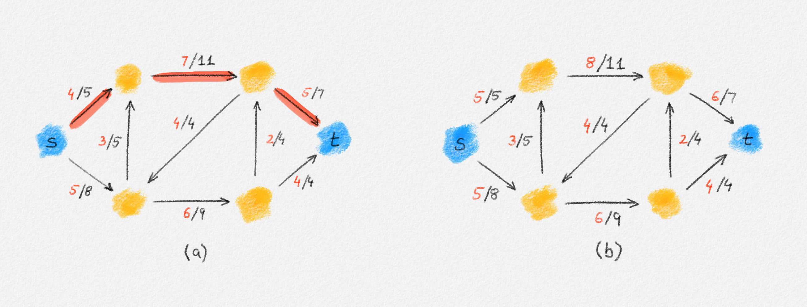
  Figure 5.2: (a) An augmenting path for the flow in Figure 5.1 that uses only edges in \(G\). (b) The flow obtained by sending one unit of flow along the path in (a).

  ---

• An augmenting path can also push flow from \(y\) to \(x\) (!) along an edge \((x,y)\) if \(f_{x,y} > 0\). Indeed, this amounts to sending some of the flow currently flowing from \(x\) to \(y\) back to \(x\), that is, reducing the flow \(f_{x,y}\) along the edge \((x,y)\) and diverting the sent-back flow to a different out-neighbour of \(x\). See Figure 5.3.

  ---

  

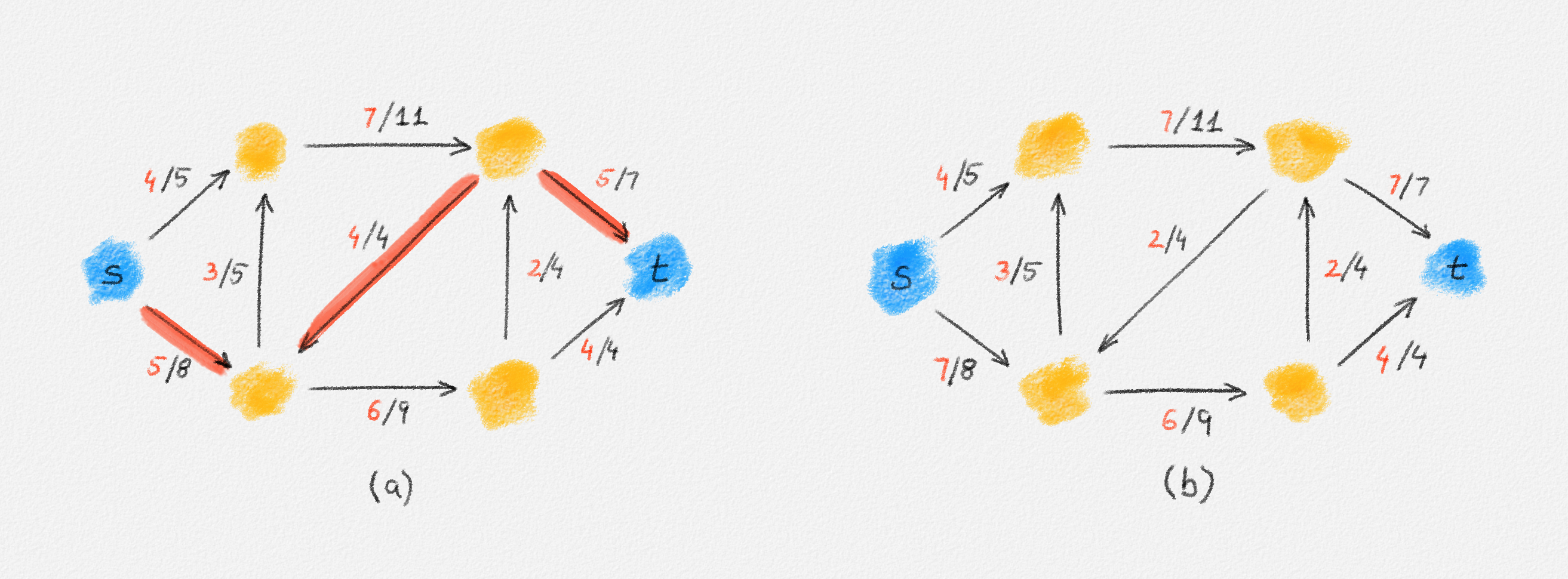
  Figure 5.3: (a) An augmenting path for the flow in Figure 5.1 that uses an edge of \(G\) in reverse. (b) The flow obtained by sending two units of flow along the path in (a).

  ---

The set of edges along which we can try to move more flow from \(s\) to \(t\) is the edge set \(E^f\) of the residual network \(G^f = \bigl(V, E^f\bigr)\) corresponding to \(f\):

The residual network of a graph \(G = (V, E)\) is the network \(G^f = \bigl(V, E^f\bigr)\), where

\[E^f = \{(x,y) \in E \mid f_{x,y} < u_e\} \cup \{(y, x) \mid (x, y) \in E \text{ and } f_{x,y} > 0\}.\]

The residual capacity of an edge \((x, y) \in E^f\) is

\[u^f_{x,y} = f_{y,x} + u_{x,y} - f_{x,y}.\]

This is illustrated in Figure 5.4.

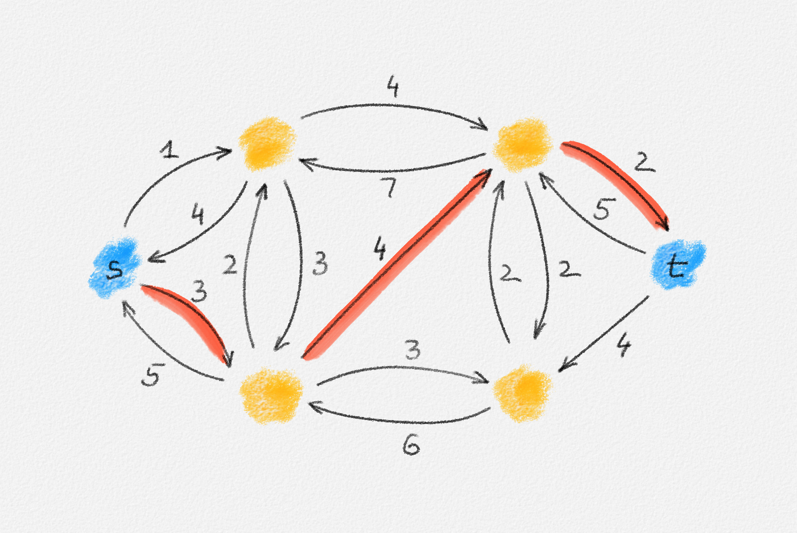
Figure 5.4: The residual network \(G^f\) corresponding to the flow in Figure 5.1. The augmenting path in Figure 5.3(a) is a directed path in \(G^f\) (red).

If \((x, y) \in E^f\) because \(f_{x,y} < u_{x,y}\), then this means that the edge \((x, y) \in E\) is not used to its full capacity and we can move up to \(u_{x,y} - f_{x,y}\) units of flow along this edge in an attempt to increase the flow from \(s\) to \(t\).

If \((x, y) \in E^f\) because \(f_{y,x} > 0\), then this means that we can move up to \(f_{y,x}\) units of flow from \(y\) back to \(x\).

It is possible that the network \(G\) contains both edges \((x, y)\) and \((y, x)\). In this case, we can move up to \(u_{x,y} - f_{x,y}\) additional units of flow from \(x\) to \(y\) along the edge \((x, y)\), and we can move up to \(f_{y,x}\) units of flow from \(x\) to \(y\) by pushing flow back along the edge \((y, x)\). This is captured by the residual capacity of the edge \((x, y)\) in \(G^f\), which is the sum of these two quantities.

With this definition of the residual network in place, we can define an augmenting path formally:

Given a feasible \(st\)-flow \(f\) in \(G\), an augmenting path \(P\) is a path from \(s\) to \(t\) in the residual network \(G^f\).

Every augmenting path algorithm starts with the trivial flow \(f_e = 0\) for all \(e \in G\) and then repeatedly finds augmenting paths along which to move more flow from \(s\) to \(t\) until there are no augmenting paths left. This is the strategy of the Ford-Fulkerson algorithm, which we discuss in Section 5.1.1. As we will see, the Ford-Fulkerson algorithm may not terminate on certain inputs. However, we will prove that it computes a maximum \(st\)-flow if it does terminate. Since all other augmenting path algorithms are variations of the Ford-Fulkerson algorithm, their correctness follows from that of the Ford-Fulkerson algorithm.

The remainder of this section is organized as follows:

• In Section 5.1.1, we discuss the Ford-Fulkerson algorithm.

• The first variation of the Ford-Fulkerson algorithm we discuss, in Section 5.1.2, is the Edmonds-Karp algorithm. Its only difference from the basic Ford-Fulkerson algorithm is that it always finds a shortest augmenting path along which to send more flow from \(s\) to \(t\). We will show that this choice of an augmenting path guarentees that the algorithm terminates, in \(O\bigl(nm^2\bigr)\) time, where \(n\) is the number of vertices and \(m\) is the number of edges in the network.

• Dinitz's algorithm is a further improvement over the Edmonds-Karp algorithm, with running time \(O\bigl(n^2m\bigr)\). We discuss this algorithm in Section 5.1.3. For dense graphs—ones where \(m = \Omega\bigl(n^2\bigr)\)—this is faster than the Edmonds-Karp algorithm by a factor of \(\Theta(n)\). One way to summarize the main idea of Dinitz's algorithm is that it finds many augmenting paths and sends flow along all of these paths simultaneously. Thus, it approaches a maximum flow faster.

5.1.1. The Ford-Fulkerson Algorithm

Every augmenting path algorithm follows the template in the following MaxFlow procedure, known as the Ford-Fulkerson algorithm. The algorithm starts with a feasible \(st\)-flow \(f\) that sends no flow along any edge. Then, as long as there exists an \(st\)-path \(P\) in \(G^f\), the algorithm sends more flow from \(s\) to \(t\) along this path \(P\). We prove below that once there is no \(st\)-path in \(G^f\), \(f\) is a maximum \(st\)-flow in \(G\). So the algorithm terminates and reports \(f\).

PROCEDURE \(\boldsymbol{\textbf{MaxFlow}(G, u, s, t)}\):

---

INPUT:

• A directed graph \(G = (V, E)\)
• A capacity labelling \(u : E \rightarrow \mathbb{R}^+\) of the edges of \(G\)
• A source vertex \(s\)
• A sink vertex \(t\)

OUTPUT:

• A maximum \(st\)-flow \(f : E \rightarrow \mathbb{R}^+\)

---

1.     Set \(f_e = 0\) for all \(e \in E\)
2.     DO FOREVER
3.         \(G^f = {}\)residual network with respect to \(f\)
4.         IF there exists an \(st\)-path \(P\) in \(G^f\) THEN
5.             \(f = \text{Augment}(G, u, f, P)\)
6.         ELSE
7.             RETURN \(f\)

The details of sending flow along an augmenting path \(P\) are implemented as a separate procedure Augment. This procedure initializes the augmented flow \(f'\) to be the same as the current flow \(f\). Then it inspects all edges in \(P\) and finds the minimum residual capacity \(\delta\) of all edges in \(P\). This is the maximum amount of flow we can send along \(P\) without violating the capacity constraint of any edge. Finally, Augment sends \(\delta\) units of flow along \(P\), by reducing the flow of any edge \((y, x)\) such that \((x, y) \in P\) by \(\min\bigl(\delta, f_{y,x}\bigr)\) and increasing the flow along any edge \((x, y)\) such that \((x, y) \in P\) by \(\max\bigl(0, \delta - f_{y,x}\bigr)\). The resulting flow \(f'\) is the new flow to be used in the next iteration of MaxFlow.

PROCEDURE \(\textbf{Augment}(G, u, f, P)\):

---

INPUT:

• A directed graph \(G = (V, E)\)
• A capacity labelling \(u : E \rightarrow \mathbb{R}^+\) of its edges
• A feasible \(st\)-flow \(f\)
• A path \(P\) in the residual network \(G^f\)

OUTPUT:

• An augmented \(st\)-flow \(f'\)

---

1.     Set \(f'_e = f_e\) for all \(e \in E\)
2.     \(\delta = \infty\)
3.     FOR ALL \((x, y) \in P\) DO
4.         \(\delta = \min\left(\delta, u^f_{x,y}\right)\)
5.     FOR ALL \((x, y) \in P\) DO
6.         \(f'_{y,x} = f_{y,x} - \min\bigl(\delta, f_{x,y}\bigr)\)
7.         \(f'_{x,y} = f_{x,y} + \max\bigl(0, \delta - f_{y,x}\bigr)\)
8.     RETURN \(f'\)

Where different augmenting path algorithms differ is in how they find augmenting paths, and this choice can have a significant impact on their running times or in fact on whether the algorithm terminates at all.

For the sake of clarity, the MaxFlow procedure constructs the residual network \(G^f\) from \(G\) and \(f\) in each iteration of the loop. An actual implementation of the algorithm initializes \(G^f = G\) at the beginning of the algorithm (because the flow is zero initially) and then, in each iteration, updates only the edges in \(G^f\) involved in the augmenting path \(P\) found in the current iteration: These are the only edges whose residual capacities or presence or absence in \(G^f\) are affected by changing the flow along the edges in \(P\).

5.1.1.1. Ford-Fulkerson May Not Terminate

The following example shows that, if the augmenting path is not chosen carefully in each iteration, then the MaxFlow procedure may not terminate and the flow value it converges to may be far from the value of a maximum flow:

Consider the network in Figure 5.5, where \(\rho = \frac{\sqrt{5}- 1}{2}\) and \(X > 2\).

Figure 5.5

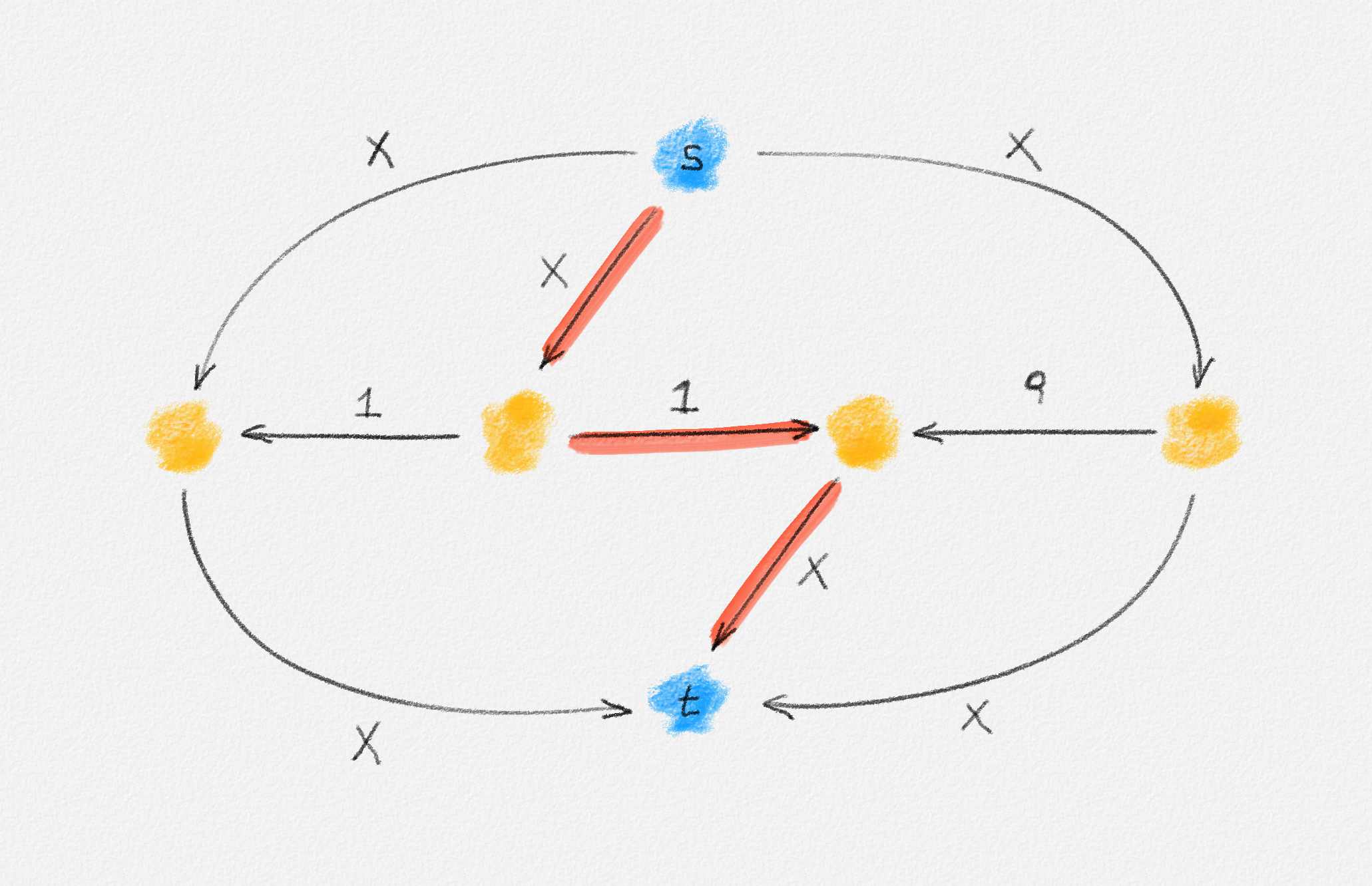
In the first augmentation, the algorithm may push one unit of flow along the red path, which leaves the residual network shown in Figure 5.6, for \(i = 1\).

Figure 5.6

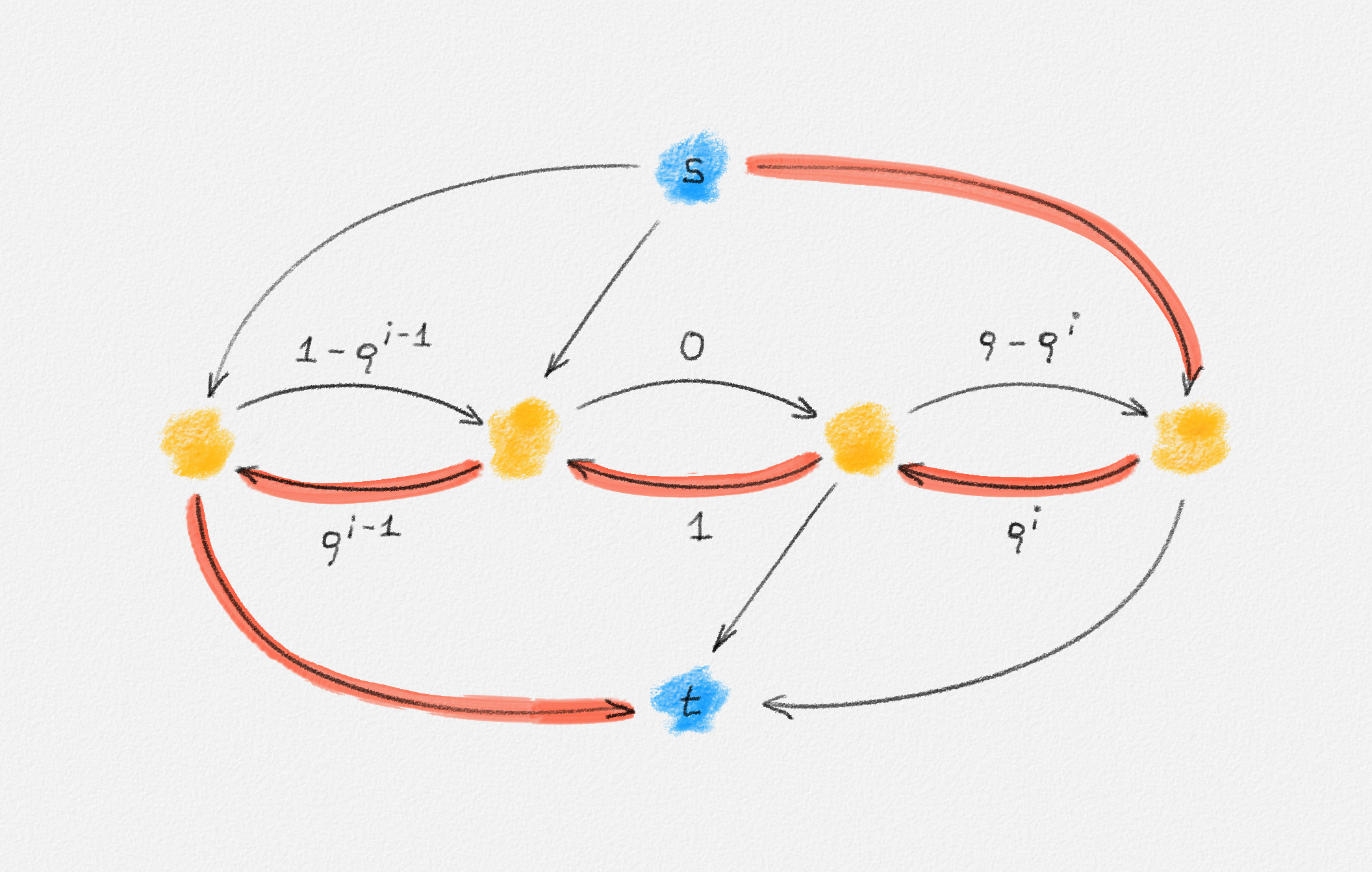
The capacities of the edges incident to \(s\) or \(t\) are not shown because \(X\) is large enough that these edges do not determine the capacity of any augmenting path used in this example.

Given the residual network in Figure 5.6 for some value \(i\), the following four augmentations return to the same residual network but with the value of \(i\) increased by \(2\):

• First, we push \(\rho^i\) units of flow along the red path in Figure 5.6. This produces the residual network in Figure 5.7.

  ---

  

  Figure 5.7

  ---

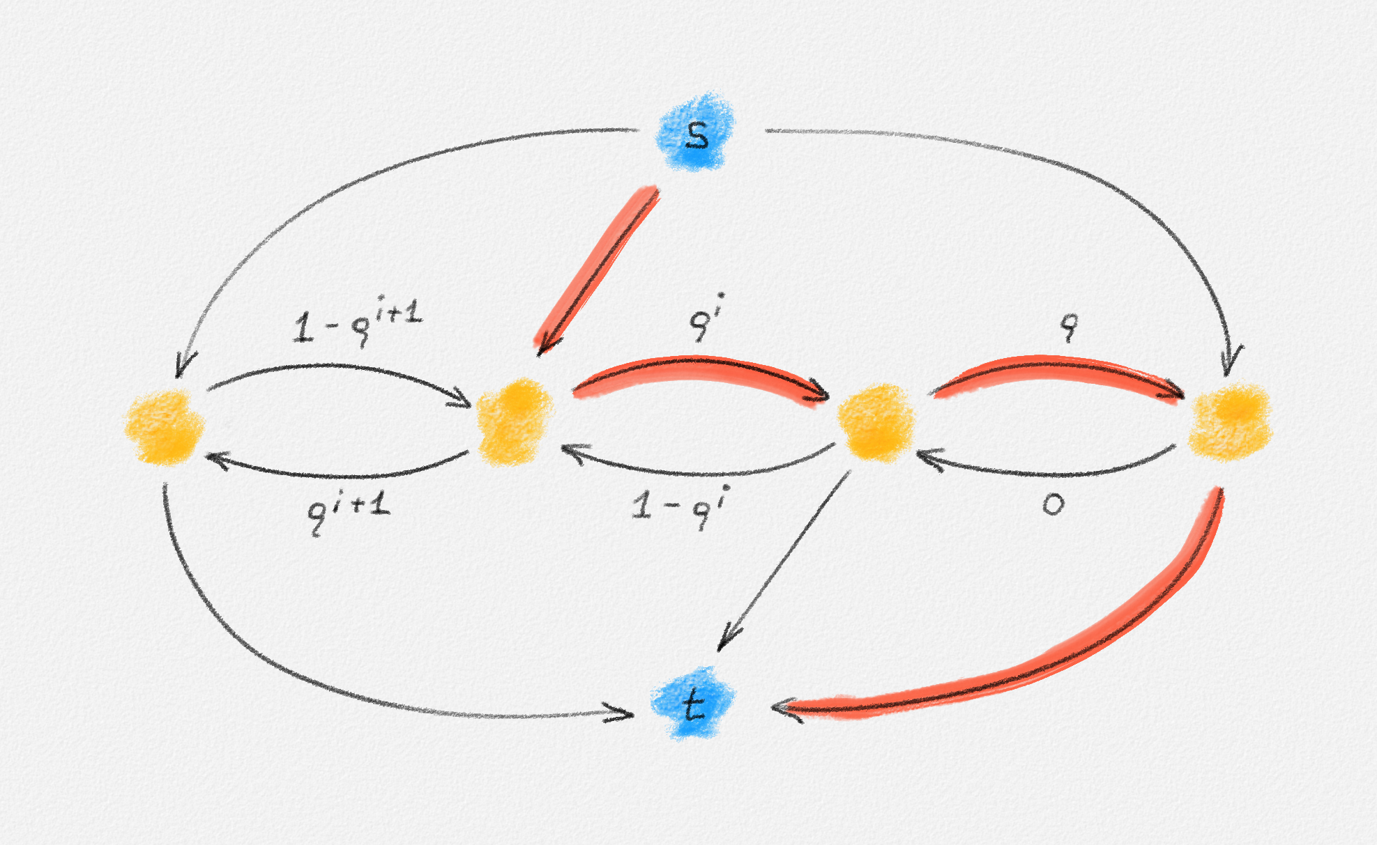
• Next, we push \(\rho^i\) units of flow along the red path in Figure 5.7. This produces the residual network in Figure 5.8.

  ---

  

  Figure 5.8

  ---

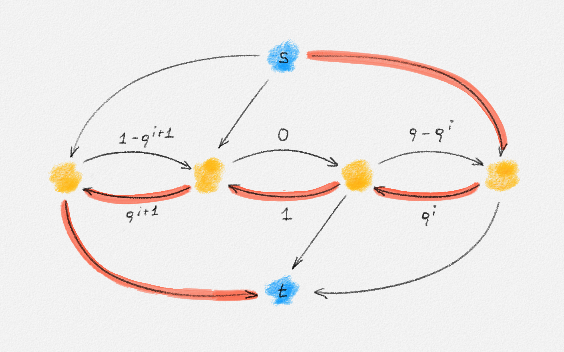
• Next, we push \(\rho^{i+1}\) units of flow along the red path in Figure 5.8. This produces the residual network in Figure 5.9.

  ---

  

  Figure 5.9

  ---

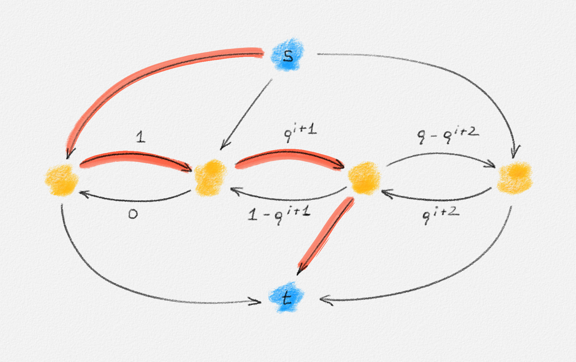
• Finally, we push \(\rho^{i+1}\) units of flow along the red path in Figure 5.9. This produces the residual network in Figure 5.6 with \(i\) increased by \(2\).

The consequence is that there always exists an augmenting path from \(s\) to \(t\), so the algorithm does not terminate. The total amount of flow pushed from \(s\) to \(t\) converges to

\[1 + \sum_{i=1}^\infty 2\rho^i = \sum_{i=0}^\infty 2\rho^i - 1 = \frac{4}{3 \sqrt{5}} - 1 < 5\]

while the maximum \(st\)-flow clearly has value \(2X + 1 > 5\). By using a large value of \(X\), the gap between the maximum \(st\)-flow and the limit of the \(st\)-flows produced by the algorithm can be made arbitrarily large.

5.1.1.2. Correctness of Ford-Fulkerson

Assume for now that the algorithm chooses augmenting paths so that its termination is guaranteed. Then the first step towards establishing the correctness of the MaxFlow procedure is to prove that each application of the Augment procedure maintains that the current flow is a feasible \(st\)-flow. Since the initial flow chosen by the MaxFlow procedure is feasible and we update the flow only by calling Augment, this ensures that the final flow returned by MaxFlow is a feasible \(st\)-flow.

Lemma 5.1: If \(f\) is a feasible \(st\)-flow in \(G\), then so is the flow \(f'\) returned by \(\boldsymbol{\textbf{Augment}(G, u, f, P)}\).

Proof: Let \(f^\delta = f' - f\), that is, for every pair of vertices \(x, y \in V\), we have

\[f^\delta_{x,y} = f'_{x,y} - f_{x,y}.\]

It's okay if theses values are negative; there is no expectation that \(f^\delta\) is a valid flow. Then

\[f^\delta_{x,y} = \begin{cases} \max\bigl(0, \delta - f_{y,x}\bigr) & \text{if } (x, y) \in P\\ -\min\bigl(\delta, f_{x, y}\bigr) & \text{if } (y, x) \in P\\ 0 & \text{otherwise.} \end{cases}\]

Since \(f\) is a valid flow, and thus satisfies flow conservation, and \(f' = f + f^\delta\), it suffices to prove that \(f^\delta\) satisfies flow conservation, in order to prove that \(f'\) satisfies flow conservation. In other words, we need to prove that

\[\sum_{y \in V} \left(f^\delta_{x,y} - f^\delta_{y,x}\right) = 0 \quad \forall x \in V \setminus \{s, t\}.\tag{5.1}\]

To prove (5.1) for all \(x \notin P\), observe that \(f^\delta_{x,y} = f^\delta_{y,x} = 0\) for all \(x \notin P\) and all \(y \in V\) because \((x, y), (y, x) \notin P\) if \(x \notin P\).

To prove (5.1) for all \(x \in P \setminus \{s, t\}\), let \(y\) be \(x\)'s predecessor in \(P\) and let \(z\) be \(x\)'s successor in \(P\). Then

\[\begin{aligned} f^\delta_{y,x} &= \max\bigl(0, \delta - f_{x, y}\bigr),\\ f^\delta_{x,y} &= -\min\bigl(\delta, f_{x, y}\bigr),\\ f^\delta_{x,z} &= \max\bigl(0, \delta - f_{z, x}\bigr),\\ f^\delta_{z,x} &= -\min\bigl(\delta, f_{z, x}\bigr),\text{ and}\\ f^\delta_{x,v} &= f^\delta_{v,x} = 0 \quad \forall v \notin \{y, z\}. \end{aligned}\]

Thus,

\[\begin{aligned} \sum_{v \in V} \left(f^\delta_{x,v} - f^\delta_{v,x}\right) &= f^\delta_{x,y} + f^\delta_{x,z} - f^\delta_{y,x} - f^\delta_{z,x}\\ &= -\min\bigl(\delta, f_{x,y}\bigr) - \max\bigl(0, \delta - f_{x,y}\bigr) + \max\bigl(0, \delta - f_{z,x}\bigr) + \min\bigl(\delta, f_{z,x}\bigr)\\ &= -\delta + \delta\\ &= 0. \end{aligned}\]

To prove that \(f'\) respects the capacity constraints, consider any pair of vertices \((x, y)\).

If \((x,y) \notin P\) and \((y,x) \notin P\), then \(0 \le f'_{x,y} = f_{x,y} \le u_{x,y}\) because \(f\) is a feasible \(st\)-flow.

If \((x,y) \in P\), then

\[0 \le \rlap{f_{y,x} - \min\bigl(\delta, f_{y,x}\bigr) \le f_{y,x} \le u_{y,x}}\phantom{\max\bigl(f_{x,y}, f_{x,y} + u_{x,y} - f_{x,y} + f_{y,x} - f_{y,x}\bigr)}\]

and

\[\begin{aligned} 0 &\le f_{x,y} \le f_{x,y} + \max\bigl(0, \delta - f_{y,x}\bigr)\\ &\le \max\bigl(f_{x,y}, f_{x,y} + u_{x,y} - f_{x,y} + f_{y,x} - f_{y,x}\bigr)\\ &= \max\bigl(f_{x,y}, u_{x,y}\bigr)\\ &= u_{x,y} \end{aligned}\]

because \(f\) is a feasible \(st\)-flow and \(\delta > 0\). Since \(f'_{x,y} = f_{x,y} + \max\bigl(0, \delta - f_{y,x}\bigr)\) and \(f'_{y,x} = f_{y,x} - \min\bigl(\delta,f_{y,x}\bigr)\), this shows that \(0 \le f'_{x,y} \le u_{x,y}\) and \(0 \le f'_{y,x} \le u_{y,x}\). Thus, \(f'\) satisfies the capacity constraints. Since it also satisfies flow conservation, \(f'\) is a feasible \(st\)-flow. ▨

Since the \(st\)-flow \(f'\) returned by Augment is feasible and sends more flow from \(s\) to \(t\) than \(f\)—\(F'_s > F_s\)—we conclude that as long as there exists an augmenting path in \(G^f\), \(f\) cannot be a maximum flow. Here is the contrapositive of this statement:

Observation 5.2: If \(f\) is a maximum \(st\)-flow in \(G\), then there exists no augmenting path from \(s\) to \(t\).

Since MaxFlow returns once there is no augmenting path in \(G^f\), to complete the correctness proof of MaxFlow, we need to prove the converse of this corollary: If there exists no augmenting path from \(s\) to \(t\) in \(G^f\), then \(f\) is a maximum \(st\)-flow. Our tool to do this is the Max-Flow Min-Cut Theorem, discussed next.

5.1.1.3. The Max-Flow Min-Cut Theorem

Recall the definition of a cut in a graph.

An \(\boldsymbol{st}\)-cut is a cut \(S\) with \(s \in S\) and \(t \notin S\). Its capacity is

\[U_S = \sum_{x \in S, y \notin S} u_{x,y}.\]

Similarly, the flow across \(S\) is

\[F_S = \sum_{x \in S, y \notin S} \bigl(f_{x,y} - f_{y,x}\bigr).\]

These definitions are illustrated in Figure 5.10.

Figure 5.10: An \(st\)-flow in a network \(G\) and an \(st\)-cut \(S\) consisting of the vertices in the shaded region. This cut has capacity \(U_S = 16\). the flow across this cut is \(F_S = 9\).

A minimum \(\boldsymbol{st}\)-cut is an \(st\)-cut of minimum capacity.

First, it is helpful to understand how \(st\)-cuts interact with flows from \(s\) to \(t\).

Lemma 5.3: Let \(S\) be an \(st\)-cut of \(G\) and let \(f\) be a feasible \(st\)-flow in \(G\). Then \(F_s = F_S\).

Proof: The lemma follows directly from flow conservation:

\[\begin{aligned} F_s &= \sum_{y \in V} \bigl(f_{s,y} - f_{y,s}\bigr)\\ &= \sum_{y \in V} \bigl(f_{s,y} - f_{y,s}\bigr) + \sum_{x \in S \setminus \{s\}}\sum_{y \in V} \bigl(f_{x,y} - f_{y,x}\bigr) \end{aligned}\]

because \(\sum_{y \in V} \bigl(f_{x,y} - f_{y,x}\bigr) = 0\) for all \(x \in S \setminus \{s\}\) due to flow conservation (\(x\) is neither \(s\), because \(x \in S \setminus \{s\}\), nor \(t\), because \(t \notin S\)). Thus,

\begin{align} F_s &= \sum_{x \in S} \sum_{y \in V} \bigl(f_{x,y} - f_{y,x}\bigr)\\ &= \sum_{x \in S} \sum_{y \in S} \bigl(f_{x,y} - f_{y,x}\bigr) + \sum_{x \in S} \sum_{y \notin S} \bigl(f_{x,y} - f_{y,x}\bigr).\tag{5.2} \end{align}

The first sum in (5.2) is \(0\) because every edge flow \(f_{x,y}\) with \(x, y \in S\) occurs twice in this sum, once with positive sign and once with negative sign. The second sum is \(F_S\). Thus, \(F_s = F_S\). ▨

The next theorem is a classical result that can be seen as the network flow equivalent of LP duality. Recall that Theorem 4.3 states that a feasible solution of an LP and a feasible solution of its dual LP are optimal solutions if and only if they have the same objective function value. The following theorem establishes an analogous relationship between maximum flows and minimum cuts.

Theorem 5.4 (Max-Flow Min-Cut Theorem): Let \(f\) be a feasible \(st\)-flow in \(G\) and let \(S\) be an \(st\)-cut of \(G\). Then \(f\) is a maximum \(st\)-flow and \(S\) is a minimum \(st\)-cut if and only if \(F_s = U_S\).

This result follows immediately from LP duality after observing that the LP formulation of the minimum \(st\)-cut problem is exactly the dual of the LP formulation of the maximum flow problem.

Exercise 5.1: Prove the Max-Flow Min-Cut Theorem by constructing the dual of the LP formulation of the maximum flow problem and showing that any feasible solution of this dual is an \(st\)-cut, and vice versa.

Here, we opt for a direct graph-theoretic proof.

Proof (Theorem 5.4): Let \(f^*\) be a maximum \(st\)-flow and let \(S^*\) be a minimum \(st\)-cut. By Lemma 5.3, we have

\[F_s \le F^*_s = F^*_{S^*} = \sum_{x \in S^*, y \notin S^*} \bigl(f^*_{x,y} - f^*_{y,x}\bigr) \le \sum_{x \in S^*, y \notin S^*} f^*_{x,y} \le \sum_{x \in S^*, y \notin S^*} u_{x,y} = U_{S^*} \le U_S.\]

Thus, if \(F_s = U_S\), then \(F_s = F^*_s = U_{S^*} = U_S\), that is, \(f\) is a maximum \(st\)-flow (\(F_s = F^*_s\)) and \(S\) is a minimum \(st\)-cut (\(U_{S^*} = U_S\)).

Conversely, assume that \(f\) is a maximum \(st\)-flow and \(S\) is a minimum \(st\)-cut. By Observation 5.2, there exists no augmenting \(st\)-path in \(G^f\). Thus, if we choose \(S'\) to be the set of all vertices reachable from \(s\) in \(G^f\), then \(s \in S'\) and \(t \notin S'\), that is, \(S'\) is an \(st\)-cut. See Figure 5.11.

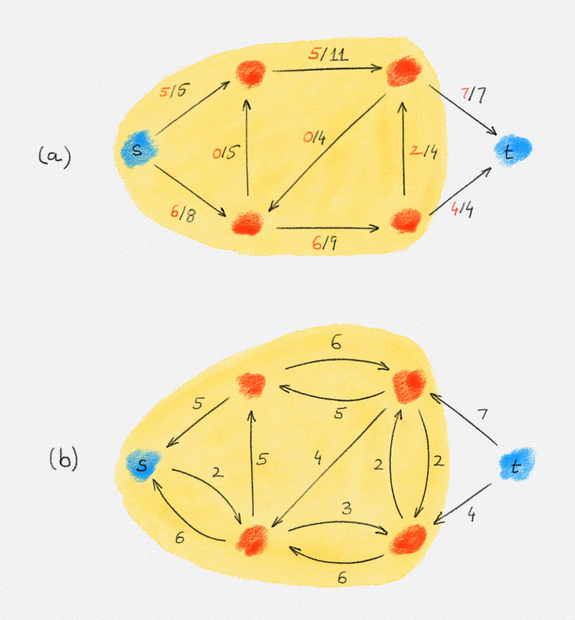
Figure 5.11: (a) A maximum flow \(f\) and a minimum cut \(S\) (shaded) that satisfy \(F_s = F_S = U_S = 11\). (b) The residual network \(G^f\). \(S\) is the set of vertices reachable from \(s\) in \(G^f\).

Since \(S\) is a minimum \(st\)-cut, we have \(F_s \le U_S \le U_{S'}\). We prove that \(F_s = U_{S'}\). Thus, \(F_s = U_S = U_{S'}\).

For every edge \((x,y) \in E\) with \(x \in S'\) and \(y \notin S'\), \(f_{x,y} = u_{x,y}\) because otherwise, the edge \((x,y)\) would be an edge of \(G^f\) and thus, since \(x \in S'\), \(y\) would also be in \(S'\). Similarly, if \(x \notin S'\) and \(y \in S'\), then \(f_{x,y} = 0\) because otherwise, the edge \((y,x)\) would belong to \(G^f\) and thus \(x \in S'\). Thus,

\[F_s = F_{S'} = \sum_{x \in S', y \notin S'} \bigl(f_{x,y} - f_{y,x}\bigr) = \sum_{x \in S', y \notin S'} u_{x,y} = U_{S'}. \text{▨}\]

The correctness of the Ford-Fulkerson algorithm now follows from the following argument: By Lemma 5.1, each iteration of the algorithm maintains that \(f\) is a feasible flow. Once the algorithm terminates, there is no more augmenting path. As in the proof of the Theorem 5.4, this implies that there exists an \(st\)-cut in \(G\) whose capacity equals \(F_s\) and, hence, \(f\) is a maximum \(st\)-flow.

What is left is to figure out an appropriate strategy to find augmenting paths that guarantees that the algorithm terminates, and hopefully quickly.

5.1.2. The Edmonds-Karp Algorithm

The Edmonds-Karp algorithm is a variation of the Ford-Fulkerson algorithm that uses what can be considered a fairly natural greedy strategy for finding an augmenting path: Run BFS from \(s\) in \(G^f\) to find a shortest \(st\)-path \(P\) in \(G^f\). An example of running the Edmonds-Karp algorithm is shown in Figure 5.12.

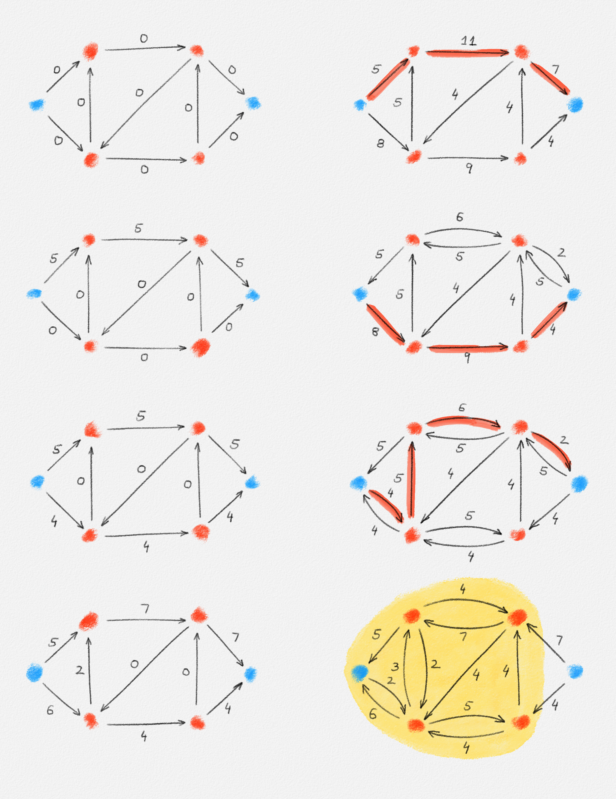
Figure 5.12: Illustration of an application of the Edmonds-Karp algorithm to the network in Figure 5.1. The edge labels in the left column show the current flow. The right column shows the corresponding residual networks and a possible path in the residual network used to augment the flow. Edge labels are residual capacities. The last residual network contains no \(st\)-path, as illustrated by the shaded cut. The corresponding flow in the bottom-left figure is thus a maximum flow in \(G\).

Since the Edmonds-Karp algorithm is a variant of the Ford-Fulkerson algorithm, it returns a maximum \(st\)-flow if it terminates. The remainder of this section is focused on proving that it does, in \(O\bigl(nm^2\bigr)\) time. The proof makes use of the following lemma:

Lemma 5.5: Let \(f\) be some \(st\)-flow in \(G\), let \(P\) be a shortest path from \(s\) to \(t\) in \(G^f\), and let \(f'\) be the \(st\)-flow obtained by applying the Augment procedure to \(f\) and \(P\). Then \(\mathrm{dist}_{G^{f'}}(s,x) \ge \mathrm{dist}_{G^f}(s,x)\) for all \(x \in V\).

In other words, as the Edmonds-Karp algorithm sends flow along augmenting paths, the shortest paths from \(s\) to all vertices in the residual network \(G^f\) become longer and longer (or at least not shorter).

Proof: Assume for the sake of contradiction that there exists a vertex \(x\) such that \(\mathrm{dist}_{G^{f'}}(s,x) < \mathrm{dist}_{G^f}(s,x)\) and choose such a vertex \(x\) with minimum distance \(\mathrm{dist}_{G^{f'}}(s,x)\). Since distances are integral, \(\mathrm{dist}_{G^{f'}}(s,x) < \mathrm{dist}_{G^f}(s,x)\) implies that

\[\mathrm{dist}_{G^{f'}}(s,v) \le \mathrm{dist}_{G^f}(s,x) - 1.\]

Let \(\Pi_{G^{f'}}(s,x)\) be a shortest path from \(s\) to \(x\) in \(G^{f'}\). Since \(\mathrm{dist}_{G^{f'}}(s,s) = 0 = \mathrm{dist}_{G^f}(s,s)\), \(x \ne s\), that is, \(x\) has a predecessor \(y\) in \(\Pi_{G^{f'}}(s,x)\). This predecessor satisfies

\[\mathrm{dist}_{G^{f'}}(s,y) = \mathrm{dist}_{G^{f'}}(s,x) - 1.\]

Thus, by the choice of \(x\),

\[\mathrm{dist}_{G^f}(s,y) \le \mathrm{dist}_{G^{f'}}(s,y) = \mathrm{dist}_{G^{f'}}(s,x) - 1 \le \mathrm{dist}_{G^f}(s,x) - 2.\tag{5.3}\]

Since every edge \((w,z) \in P\) satisfies

\[\mathrm{dist}_{G^f}(s,z) = \mathrm{dist}_{G^f}(s,w) + 1,\]

this implies that \((x,y) \notin P\) and \((y,x) \notin P\). In particular, \(f'_{x,y} = f_{x,y}\) and \(f'_{y,x} = f_{y,x}\). Thus, since \((y,x) \in G^{f'}\), \((y,x)\) is also an edge in \(G^f\), a contradiction because this would imply that

\[\mathrm{dist}_{G^f}(s,x) \le \mathrm{dist}_{G^f}(s,y) + 1,\]

but we observed in (5.3) that

\[\mathrm{dist}_{G^f}(s,x) \ge \mathrm{dist}_{G^f}(s,y) + 2.\ \text{▨}\]

Theorem 5.6: The Edmonds-Karp algorithm computes a maximum flow in \(O\bigl(nm^2\bigr)\) time.

Proof: As already observed, the correctness of the Edmonds-Karp algorithm follows because it is a variant of the Ford-Fulkerson algorithm. Next, we analyze its running time.

Constructing \(G^f\), running BFS in \(G^f\), and applying the Augment procedure to the path \(P\) found by the BFS takes \(O(m)\) time. Thus, it suffices to show that the algorithm terminates after at most \(nm\) iterations.

Let \(f^{(0)}, \ldots, f^{(r)}\) be the sequence of flows constructed by the algorithm. For \(0 \le i < r\), let \(P^{(i)}\) be the augmenting path used to produce \(f^{(i+1)}\) from \(f^{(i)}\) and let \(\delta^{(i)} = F^{(i+1)}_s - F^{(i)}_s\) be the amount of flow sent along this path. An edge \((x,y) \in E^{f^{(i)}}\) is critical for the augmenting path \(P^{(i)}\) if \((x,y) \in P^{(i)}\) and \(u^{f^{(i)}}_{x,y} = \delta^{(i)}\). In other words, the edge \((x,y)\) is one of the edges that limit the amount of flow sent along \(P^{(i)}\) to be no more than \(\delta^{(i)}\). Let \(E' = \{(x, y), (y, x) \mid (x, y) \in E\}\) be the set of edges in \(G\) and their reversals. We have \(|E'| \le 2m\) and every residual network \(G^{f^{(i)}} = \bigl(V, E^{f^{(i)}}\bigr)\) satisfies \(E^{f^{(i)}} \subseteq E'\). Thus, it suffices to show that every edge in \(E'\) is critical for at most \(\frac{n}{2}\) paths. Since every augmenting path \(P^{(i)}\) has at least one critical edge, this implies that \(r \le nm\), that is, the algorithm runs for at most \(nm\) iterations.

Consider an edge \((x, y) \in E'\) and two indices \(i < j\) such that \((x,y)\) is critical for \(P^{(i)}\) and \(P^{(j)}\) but not for any path \(P^{(h)}\) with \(i < h < j\). Then

\[\delta^{(i)} = u^{f^{(i)}}_{x,y} = u_{x,y} - f^{(i)}_{x,y} + f^{(i)}_{y,x} \ge f^{(i)}_{y,x}.\]

Thus,

\[f^{(i+1)}_{y,x} = f^{(i)}_{y,x} - \min\Bigl(\delta^{(i)},f^{(i)}_{y,x}\Bigr) = 0\]

and

\[\begin{aligned} f^{(i+1)}_{x,y} &= f^{(i)}_{x,y} + \max\Bigl(0, \delta^{(i)} - f^{(i)}_{y,x}\Bigr)\\ &= f^{(i)}_{x,y} + u_{x,y} - f^{(i)}_{x,y} + f^{(i)}_{y,x} - f^{(i)}_{y,x}\\ &= u_{x,y}. \end{aligned}\]

Therefore, \((x,y) \notin G^{f^{(i+1)}}\). Since \((x,y) \in P^{(j)}\), it does belong to \(G^{f^{(j)}}\). Thus, there exists a minimum index \(k > i + 1\) such that \((x,y) \in G^{f^{(k)}}\). Since \((x,y) \in G^{f^{(k)}}\) and \((x,y) \notin G^{f^{(k-1)}}\), the augmentation of \(f^{(k-1)}\) to produce \(f^{(k)}\) must push some flow from \(y\) to \(x\), that is, \((y,x) \in P^{(k-1)}\).

By Lemma 5.5,

\[\mathrm{dist}_{G^{f^{(k-1)}}}(s,y) \ge \mathrm{dist}_{G^{f^{(i)}}}(s,y).\tag{5.4}\]

Since \((y,x) \in P^{(k-1)}\) and \(P^{(k-1)}\) is a shortest path from \(s\) to \(t\) in \(G^{f^{(k-1)}}\),

\[\mathrm{dist}_{G^{f^{(k-1)}}}(s,x) = \mathrm{dist}_{G^{f^{(k-1)}}}(s,y) + 1.\tag{5.5}\]

By Lemma 5.5 again,

\[\mathrm{dist}_{G^{f^{(j)}}}(s,x) \ge \mathrm{dist}_{G^{f^{(k-1)}}}(s,x).\tag{5.6}\]

Since \((x,y) \in P^{(j)}\) and \(P^{(j)}\) is a shortest path from \(s\) to \(t\) in \(G^{f^{(j)}}\),

\[\mathrm{dist}_{G^{f^{(j)}}}(s,y) = \mathrm{dist}_{G^{f^{(j)}}}(s,x) + 1.\tag{5.7}\]

The combination of (5.4)–(5.7) shows that

\[\mathrm{dist}_{G^{f^{(j)}}}(s,y) \ge \mathrm{dist}_{G^{f^{(i)}}}(s,y) + 2.\]

Since every vertex \(y\) reachable from \(s\) in \(G^{f^{(h)}}\) satisfies \(\mathrm{dist}_{G^{f^{(h)}}}(s,y) \le n\), for all \(0 \le h < r\), this implies that the edge \((x,y)\) is critical for at most \(\frac{n}{2}\) of the paths \(P^{(0)}, \ldots, P^{(r-1)}\). ▨

5.1.3. Dinitz's Algorithm*

What prevents the Edmonds-Karp algorithm from achieving a better running time is that it constructs \(G^f\) and uses a full BFS of \(G^f\) to find the augmenting path in each iteration. Dinitz's algorithm follows the same basic idea of increasing the current flow by pushing more flow along augmenting paths, but it uses a single BFS to find potentially many augmenting paths. As we will see, this reduces its running time to \(O\bigl(n^2m\bigr)\).

Running BFS in \(G^f\) labels every vertex \(x\) in \(G^f\) with its distance \(\mathrm{dist}_{G^f}(s,x)\).

The level graph \(L^f \subseteq G^f\) (see Figure 5.13) is obtained from \(G^f\) by deleting all edges \((x,y)\) such that \(\mathrm{dist}_{G^f}(s,y) \le \mathrm{dist}_{G^f}(s,x)\).

It is easy to see that \(\mathrm{dist}_{G^f}(s,x) = \mathrm{dist}_{L^f}(s,x)\) for all \(x \in V\). This distance is called the level of \(x\) in \(G^f\).

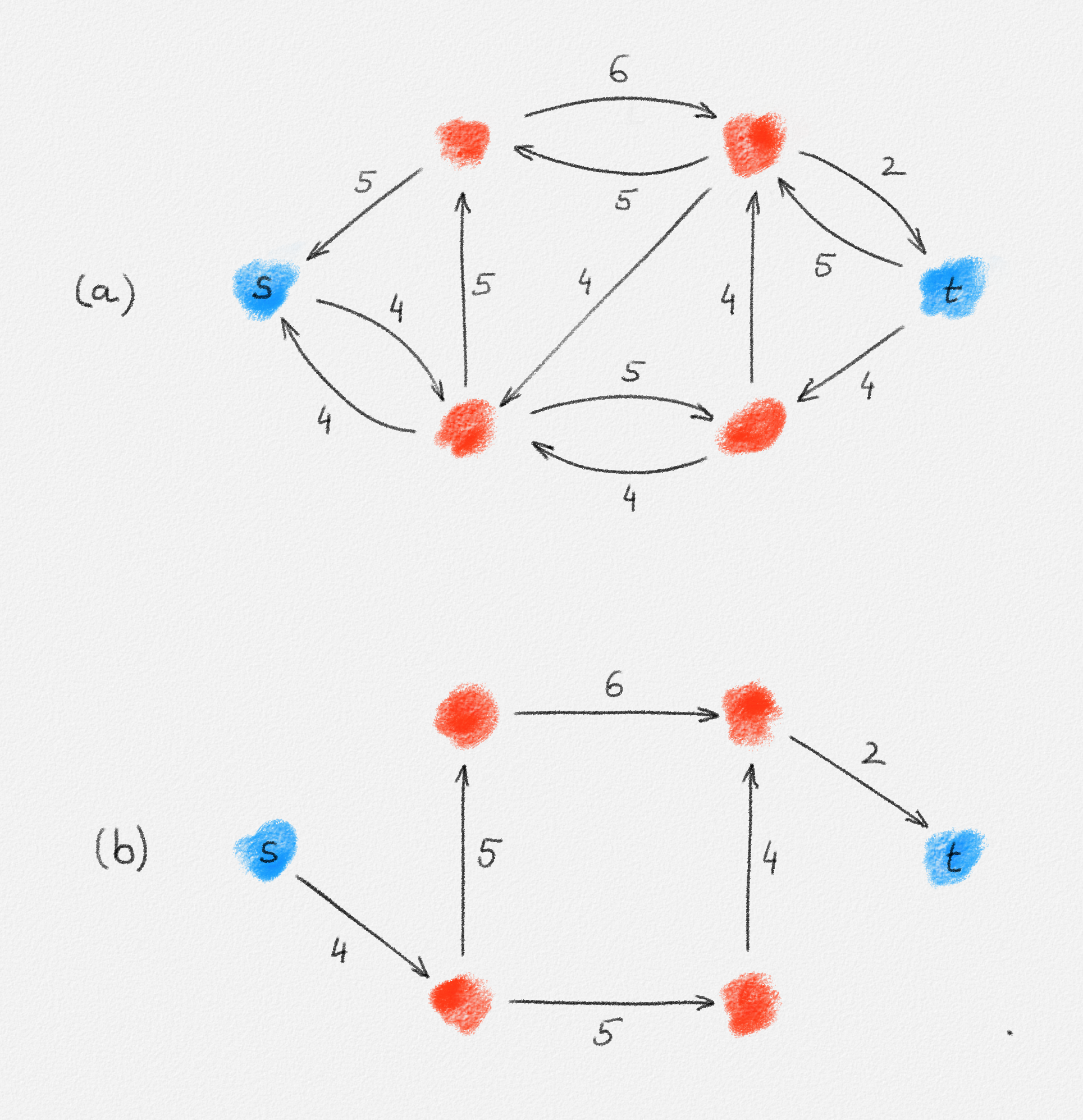
Figure 5.13: (a) A residual network. (b) The corresponding level graph.

Let \(\ell^f\) be \(t\)'s level in \(G^f\). The idea of Dinitz's algorithm is to spend \(O(nm)\) time to find a new \(st\)-flow \(f'\) with \(\ell^{f'} > \ell^f\) in each iteration. As long as there exists an augmenting path from \(s\) to \(t\) in the current residual network \(G^f\), \(\ell^f \le n\). Thus, the algorithm runs for at most \(n\) iterations, each with cost \(O(nm)\), giving a running time of \(O\bigl(n^2 m\bigr)\), which is better than \(O\bigl(nm^2\bigr)\) unless \(G\) is sparse. An illustration of Dinitz's algorithm is given in Figure 5.15.

Let \(b\) be a feasible \(st\)-flow in \(L^f\). Any such flow \(b\) defines a new \(st\)-flow \(f'\) in \(G\) as

\[f'_{x,y} = \begin{cases} f_{x,y} - \min\bigl(b_{y,x},f_{x,y}\bigr) & \text{if } (y,x) \in L^f\\ f_{x,y} + \max\bigl(0,b_{x,y} - f_{y,x}\bigr) & \text{if } (x,y) \in L^f\\ f_{x,y} & \text{otherwise.} \end{cases}\tag{5.8}\]

The next lemma shows that \(f'\) is once again a feasible \(st\)-flow in \(G\).

Lemma 5.7: If \(f\) is a feasible \(st\)-flow in \(G\) and \(b\) is a feasible \(st\)-flow in \(L^f\), then the flow \(f'\) defined in (5.8) is also a feasible \(st\)-flow in \(G\).

Proof: The proof is very similar to the proof of Lemma 5.1. Let \(f^\delta = f' - f\). Then

\[f^\delta_{x, y} = \begin{cases} \max\bigl(0, b_{x, y} - f_{y, x}\bigr) & \text{if } (x, y) \in L^f\\ -\min\bigl(b_{y, x}, f_{x, y}\bigr) & \text{if } (y, x) \in L^f\\ 0 & \text{otherwise.} \end{cases}\]

If \((x, y) \in L^f\), this implies that

\[\begin{aligned} f^\delta_{x, y} - f^\delta_{y, x} &= \max\bigl(0, b_{x, y} - f_{y, x}\bigr) + \min\bigl(b_{x, y}, f_{y, x}\bigr)\\ &= b_{x, y}\\ &= b_{x, y} - b_{y, x} \end{aligned}\]

because \(b_{y, x} = 0\). If both \((x, y), (y, x) \notin L^f\), then

\[f^\delta_{x, y} = f^\delta_{y, x} = b_{x, y} = b_{y, x} = 0,\]

so once again

\[f^\delta_{x, y} - f^\delta_{y, x} = b_{x, y} - b_{y, x}.\]

Thus,

\[\begin{aligned} \sum_{y \in V} \bigl(f'_{x, y} - f'_{y, x}\bigr) &= \sum_{y \in V} \bigl(f_{x, y} - f_{y, x}\bigr) + \sum_{y \in V} \Bigl(f^\delta_{x, y} - f^\delta_{y, x}\Bigr)\\ &= \sum_{y \in V} \bigl(f_{x, y} - f_{y, x}\bigr) + \sum_{y \in V} \bigl(b_{x, y} - b_{y, x}\bigr) = 0 \quad \forall x \in V \setminus \{s, t\} \end{aligned}\]

because both \(f\) and \(b\) are feasible \(st\)-flows. This shows that \(f'\) satisfies flow conservation.

To prove that \(f'\) satisfies the capacity constraints, consider any pair of vertices \((x,y)\).

If \((x,y) \notin L^f\) and \((y,x) \notin L^f\), then

\[0 \le f'_{x,y} = f_{x,y} \le u_{x,y}\]

because \(f\) is a feasible flow.

If \((x,y) \in L^f\), then

\[0 \le f_{y,x} - \min\bigl(b_{x,y}, f_{y,x}\bigr) \le f_{y,x} \le u_{y,x}\]

and

\[\begin{aligned} 0 &\le f_{x,y} \le f_{x,y} + \max\bigl(0, b_{x,y} - f_{y,x}\bigr)\\ &\le \max\left(f_{x,y}, f_{x,y} + u^f_{x,y} - f_{y,x}\right)\\ &= \max\bigl(f_{x,y}, f_{x,y} + u_{x,y} - f_{x,y} + f_{y,x} - f_{y,x}\bigr)\\ &= \max\bigl(f_{x,y}, u_{x,y}\bigr)\\ &= u_{x,y} \end{aligned}\]

because \(f\) and \(b\) are feasible \(st\)-flows in \(G\) and \(L^f\), respectively. Since \(f'_{x,y} = f_{x,y} + \max\bigl(0, b_{x,y} - f_{y,x}\bigr)\) and \(f'_{y,x} = f_{y,x} - \min\bigl(b_{x,y}, f_{y,x}\bigr)\), this shows that \(0 \le f'_{x,y} \le u_{x,y}\) and \(0 \le f'_{y,x} \le u_{y,x}\). Thus, \(f'\) satisfies the capacity constraints. Since it also satisfies flow conservation, it is a feasible \(st\)-flow. ▨

The key to guaranteeing that Dinitz's algorithm terminates after at most \(n\) iterations is to find the right kind of flow in \(L^f\), one that ensures that \(\ell^{f'} > \ell^f\). Next we define such a flow and show how to find it efficiently.

5.1.3.1. Blocking Flows

Let \(L^{f,b}\) be the residual network of \(L^f\) w.r.t. some flow \(b\) in \(L^f\).

A path \(P\) in \(L^{f,b}\) is called monotone if every edge \((x,y) \in P\) satisfies \(\mathrm{dist}_{G^f}(s,x) < \mathrm{dist}_{G^f}(s,y)\), that is, if it is an edge of \(L^f\).

A feasible \(st\)-flow \(b\) in \(L^f\) is called a blocking flow if \(L^{f,b}\) has no monotone path. See Figure 5.14.

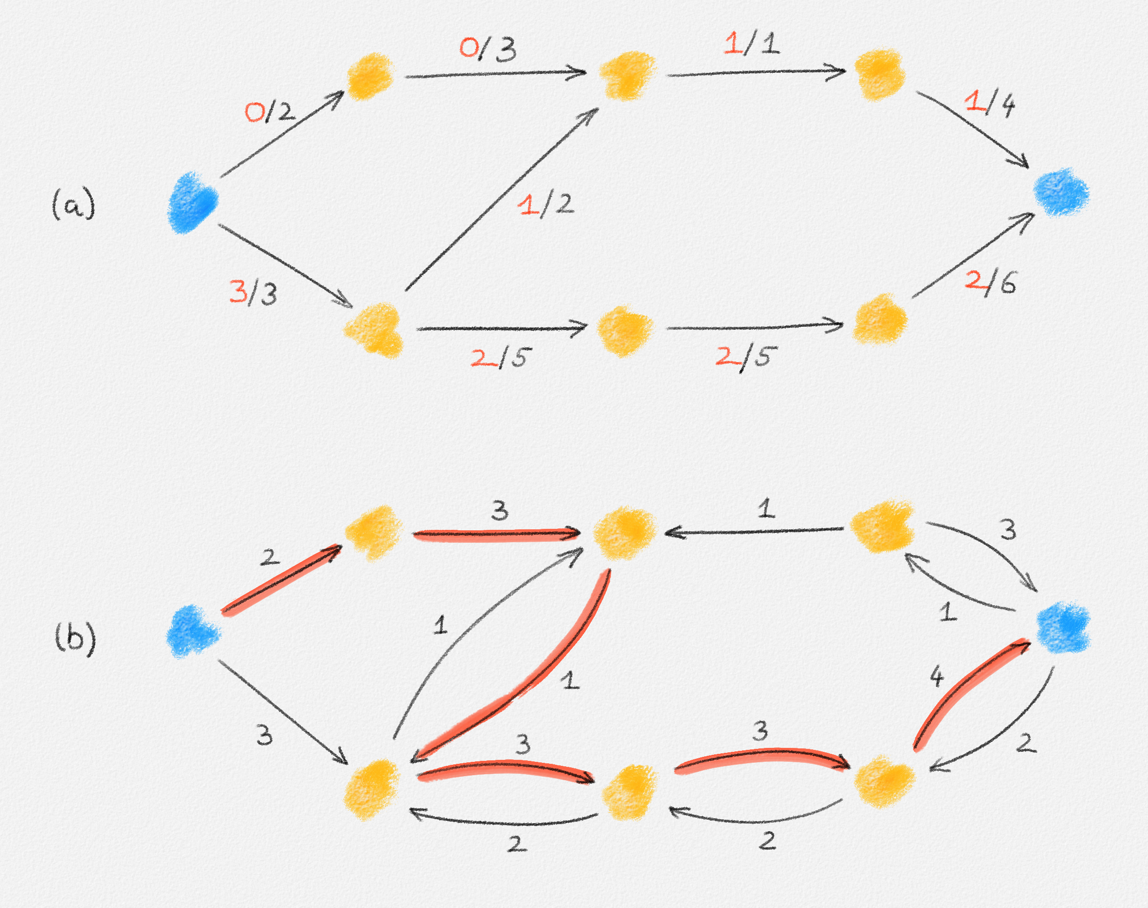
Figure 5.14: The flow represented by the red edge labels in (a) is a blocking flow. Black edge labels are capacities. While there exists an augmenting path in the residual network (b), shown in red, that path is not monotone.

Figure 5.15: Illustration of an application of Dinitz's algorithm to the network in Figure 5.1. The edge labels in the left column show the current flow. The middle column shows the corresponding residual networks. Edge labels are residual capacities. The right column shows the level graph and a blocking flow used to augment the current flow to obtain the next flow. The red edge labels represent the blocking flow, the black edge labels the residual capacities. The last residual network contains no \(st\)-path, as illustrated by the shaded cut. This is even more visible in the level graph, which is disconnected. The corresponding flow in the bottom-left figure is thus a maximum flow in \(G\).

Lemma 5.8: Let \(b\) be a blocking flow in \(L^f\). Then the \(st\)-flow \(f'\) defined in (5.8) satisfies \(\ell^{f'} > \ell^f\).

Proof: Assume the contrary and let \(P = \langle s = x_0, \ldots, x_{\ell^{f'}} = t \rangle\) be a shortest path from \(s\) to \(t\) in \(G^{f'}\). First observe that

\[\mathrm{dist}_{G^f}(s,x_i) \le \mathrm{dist}_{G^f}(s,x_{i-1}) + 1\]

for all \(1 \le i \le \ell^{f'}\). Indeed, if there existed an index \(i\) such that

\[\mathrm{dist}_{G^f}(s,x_i) > \mathrm{dist}_{G^f}(s,x_{i-1}) + 1,\]

then this would imply that \((x_{i-1},x_i) \notin L^f\) and \((x_i,x_{i-1}) \notin L^f\). Since \(f'_{x,y} \ne f_{x,y}\) only for edges \((x,y)\) such that \((x,y) \in L^f\) or \((y,x) \in L^f\), this would imply that \(f'_{x_{i-1},x_i} = f_{x_{i-1},x_i}\) and \(f'_{x_i,x_{i-1}} = f_{x_i, x_{i-1}}\). Since \((x_{i-1},x_i) \in G^{f'}\), this would imply that \((x_{i-1},x_i) \in G^f\) and, therefore,

\[\mathrm{dist}_{G^f}(s,x_i) \le \mathrm{dist}_{G^f}(s,x_{i-1}) + 1,\]

a contradiction.

Since

\[\begin{aligned} \mathrm{dist}_{G^f}(s,x_0) &= \mathrm{dist}_{G^f}(s,s) = 0,\\ \mathrm{dist}_{G^f}\bigl(s,x_{\ell^{f'}}\bigr) &= \mathrm{dist}_{G^f}(s,t) = \ell_f,\ \text{and}\\ \mathrm{dist}_{G^f}(s,x_i) &\le \mathrm{dist}_{G^f}(s,x_{i-1}) + 1 && \forall 1 \le i \le \ell^{f'}, \end{aligned}\]

the path \(P\) has length at least \(\ell^f\).

If it includes at least one edge \((x_{i-1},x_i)\) with \(\mathrm{dist}_{G^f}(s,x_i) \le \mathrm{dist}_{G^f}(s,x_{i-1})\), its length is strictly greater than \(\ell^f\), that is, \(\ell^{f'} > \ell^f\), as claimed by the lemma.

So assume that

\[\mathrm{dist}_{G^f}(s,x_i) = \mathrm{dist}_{G^f}(s,x_{i-1}) + 1 \quad \forall 1 \le i \le \ell^{f'}.\]

Since \(f'\) is obtained from \(f\) and \(b\) using (5.8) and for every edge \((x,y) \in L^f\),

\[\mathrm{dist}_{G^f}(s,y) = \mathrm{dist}_{G^f}(s,x) + 1,\]

we have

• \(f'_{x,y} \ge f_{x,y}\) for every edge \((x,y) \in G\) with \(\mathrm{dist}_{G^f}(s,y) = \mathrm{dist}_{G^f}(s,x) + 1\),
• \(f'_{x,y} \le f_{x,y}\) for every edge \((x,y) \in G\) with \(\mathrm{dist}_{G^f}(s,y) = \mathrm{dist}_{G^f}(s,x) - 1\), and
• \(f'_{x,y} = f_{x,y}\) for any other edge.

Thus, any edge \((x,y) \in G^{f'}\) with \(\mathrm{dist}_{G^f}(s,y) = \mathrm{dist}_{G^f}(s,x) + 1\) satisfies \(u^f_{x,y} \ge u^{f'}_{x,y} > 0\), that is, the edge also belongs to \(G^f\), and hence to \(L^f\). This shows that \(P\) is a path in \(L^f\).

For every edge \((x_{i-1},x_i) \in P\), \(u^{f'}_{x_{i-1},x_i} > 0\). Also,

\[\begin{aligned} f'_{x_{i-1},x_i} &= f_{x_{i-1},x_i} + \max\bigl(0, b_{x_{i-1},x_i} - f_{x_i,x_{i-1}}\bigr)\\ f'_{x_i,x_{i-1}} &= f_{x_i,x_{i-1}} - \min\bigl(b_{x_{i-1},x_i}, f_{x_i,x_{i-1}}\bigr). \end{aligned}\]

Thus,

\[\begin{aligned} 0 &< u^{f'}_{x_{i-1},x_i}\\ &= u_{x_{i-1},x_i} - f'_{x_{i-1},x_i} + f'_{x_i,x_{i-1}}\\ &= u_{x_{i-1},x_i} - f_{x_{i-1},x_i} - \max\bigl(0, b_{x_{i-1},x_i} - f_{x_i,x_{i-1}}\bigr) + f_{x_i,x_{i-1}} - \min\bigl(b_{x_{i-1},x_i}, f_{x_i,x_{i-1}}\bigr)\\ &= u^f_{x_{i-1},x_i} - b_{x_{i-1},x_i}, \end{aligned}\]

that is,

\[b_{x_{i-1},x_i} < u^f_{x_{i-1},x_i}.\]

Since this is true for every edge \((x_{i-1},x_i) \in P\), \(P\) is a path in \(L^{f,b}\). Since \(P\) is monotone, this shows that \(b\) is not a blocking flow in \(L^f\), a contradiction. ▨

By Lemma 5.8, augmenting \(f\) using a blocking flow in each iteration of the algorithm ensures that \(\ell^f\) increases in each iteration and thus, as argued before, that the algorithm runs for at most \(n\) iterations. To achieve the desired running time of \(O\bigl(n^2m\bigr)\), it thus suffices to show how to find a blocking flow in \(O(nm)\) time. This is the final piece in the puzzle, which we discuss next.

5.1.3.2. Finding a Blocking Flow

Lemma 5.9: A blocking flow in \(L^f\) can be found in \(O(nm)\) time.

Proof: To find a blocking flow \(b\) in \(L^f\), Dinitz's algorithm essentially applies the Ford-Fulkerson algorithm to \(L^f\), but with two twists:

First, instead of looking for arbitrary augmenting paths in the residual network \(L^{f,b}\), we only look for monotone augmenting paths. By definition, once we cannot find such a path, \(b\) is a blocking flow even if there exist other (non-monotone) augmenting paths in \(L^{f,b}\).

This allows us to get away with maintaining only part of \(L^{f,b}\): Since we never use backward edges in \(L^{f,b}\)—edges \((x,y)\) that satisfy \(\mathrm{dist}_{G^f}(s, x) = \mathrm{dist}_{G^f}(s, y) + 1\)—we do not need to construct them. The forward edges in \(L^{f,b}\) are edges of \(L^f\). Thus, we initialize \(L^{f,b} = L^f\) because the initial flow is \(b = 0\). As we saturate edges in \(L^{f,b}\)—we send \(u^{f,b}_e\) flow along an edge \(e \in L^{f,b}\)—we simply remove them.

Maintaining \(L^{f,b}\) as the subgraph of forward edges in the residual network of \(b\) has the advantage that a path in the residual network of \(b\) is monotone if and only if it is a path in \(L^{f,b}\). Thus, we can look for any \(st\)-path in \(L^{f,b}\). Once we do not find such a path, \(b\) is a blocking flow.

How often do we need to augment \(b\) before it becomes a blocking flow? Note that \(L^f\) has at most \(m\) edges: For every edge \((x,y)\) of \(G\), \(G^f\) may contain both edges \((x,y)\) and \((y,x)\), but at most one of them can be a forward edge. Since we initialize \(L^{f,b} = L^f\), \(L^{f,b}\) starts out with at most \(m\) edges. Each augmentation of \(b\) along some path \(P\) in \(L^{f,b}\) saturates at least one edge in \(P\). This edge is removed from \(L^{f,b}\). Thus, \(L^{f,b}\) has no edges left after at most \(m\) augmentations. At this point, \(b\) is obviously a blocking flow. Thus, it takes at most \(m\) augmentations of \(b\) to obtain a blocking flow in \(L^f\).

If we could find each monotone \(st\)-path in \(L^{f,b}\) used to augment \(b\) in \(O(n)\) time, finding a blocking flow would take \(O(nm)\) time as claimed because we just observed that we need to find at most \(m\) such paths. Finding these paths is the only hard part; given a monotone \(st\)-path \(P\) in \(L^{f,b}\), we can easily augment \(b\) in \(O(n)\) time: Since \(P\) is monotone, it has \(\ell^f \le n - 1\) edges. Inspecting all of these edges to find the one with minimum residual capacity \(u^{f,b}_e = \delta\) takes \(O(n)\) time. We can then inspect each edge in \(P\) a second time to increase the flow along it and decrease its residual capacity by \(\delta\). Any edge whose residual capacity becomes \(0\) is removed.

Unfortunately, finding a single monotone \(st\)-path in \(L^{f,b}\) may take much longer than \(O(n)\) time. Here is the second twist in the algorithm, which ensures that the algorithm nevertheless takes \(O(nm)\) time overall: We use depth-first search to find \(st\)-paths in \(L^{f,b}\), and we terminate each search as soon as we find a path from \(s\) to \(t\).

Let \(P_1, \ldots, P_r\) be the \(st\)-paths in \(L^{f,b}\) used to construct \(b\). We can divide the edges inspected to find each path \(P_i\) into two subsets: those in \(P_i\) and those not in \(P_i\). \(P_i\) has \(\ell^f \le n - 1\) edges. Let \(m_i\) be the number of inspected edges not in \(P_i\). Then finding \(P_i\) takes \(O(n + m_i)\) time. The cost of finding all paths \(P_1, \ldots, P_r\) is thus \(O\bigl(nm + \sum_{i=1}^r m_i\bigr)\) because \(r \le m\). Next we prove that we can ensure that \(\sum_{i=1}^r m_i \le m\). Thus, the overall running time of the algorithm for finding a blocking flow is \(O(nm)\), as claimed.

Consider the construction of \(P_i\). The key observation is that the \(m_i\) edges not in \(P_i\) that are inspected during the construction of \(P_i\) can be removed from \(L^{f,b}\) because they cannot belong to any \(st\)-path in \(L^{f,b}\). By removing these edges, we ensure that every edge of \(L^f\) is inspected during the construction of at most one path \(P_i\) without being part of this path. Thus, \(\sum_{i=1}^r m_i \le m\) follows immediately.

So let \(e\) be an edge not in \(P_i\) that is inspected during the construction of \(P_i\). Since we terminate the search for \(P_i\) as soon as we find the last edge of \(P_i\), that is, as soon as we reach \(t\), \(e\) is inspected before the last edge in \(P_i\). Since \(e \notin P_i\), this means that the depth-first search followed \(e\) and then backtracked across \(e\) before finding \(P_i\). In particular, the depth-first search explored all edges reachable from \(e\) without reaching \(t\). Thus, \(e\) is not part of any \(st\)-path in \(L^{f,b}\) at the time we construct \(P_i\). Since we never add any edge to \(L^{f,b}\), \(e\) cannot be part of any \(st\)-path in any subsequent iteration either, so \(e\) can safely be removed from \(L^{f,b}\). ▨

We have shown that a blocking flow can be found in \(O(nm)\) time, that augmenting a feasible \(st\)-flow with a blocking flow produces another feasible \(st\)-flow, and that at most \(n\) such augmentations are necessary to obtain a maximum \(st\)-flow. Thus, we have shown the following theorem:

Theorem 5.10: Dinitz's algorithm computes a maximum \(st\)-flow in \(O\bigl(n^2m\bigr)\) time.

5.2. Preflow-Push Algorithms

The main characteristic of augmenting path algorithms is that they maintain the invariant that the current \(st\)-flow \(f\) is feasible at any point in the algorithm. They use augmenting paths to increase the flow while maintaining feasibility. Preflow-push algorithms approach the problem from a different angle: Clearly, the maximum amount of flow that could possibly be moved from \(s\) to \(t\) is

\[\sum_{y \in V} u_{s,y},\]

the total capacity of \(s\)'s out-edges. So the algorithm is optimistic and pushes exactly \(u_{s,y}\) units of flow along every out-edge \((s,y)\) of \(s\), hoping that it will eventually be able to move all this flow to \(t\). At this point, \(s\)'s out-neighbours do not satisfy flow conservation, so the algorithm tries to re-establish flow conservation by pushing the flow each neighbour \(y\) receives from \(s\) on to its out-neighbours. If \(y\)'s out-edges have sufficient capacity, this restores flow conservation at \(y\) but now creates an excess of flow at \(y\)'s out-neighbours. By pushing flow along in this fashion, a certain amount of flow eventually reaches \(t\) while some nodes in \(G\) may still be left with an excess flow they were not able to pass on to any of their out-neighbours. This flow is sent back to \(s\) to restore flow conservation, at which point the resulting flow is feasible and, as we show below, maximum if the algorithm is implemented correctly.

The first part of the name of these algorithms stems from the following definition:

A preflow is a function \(f: E \rightarrow \mathbb{R}\) such that

\[0 \le f_e \le u_e \quad \forall e \in E\]

and

\[\sum_{y \in V} \bigl(f_{y,x} - f_{x,y}\bigr) \ge 0 \quad \forall x \in V \setminus \{ s, t \}.\]

In other words, \(f\) satisfies the capacity constraints and no vertex other than \(s\) or \(t\) generates any flow.

Every preflow-push algorithm initializes the preflow by setting

\[f_{x,y} = \begin{cases} u_{x,y} & \text{if } x = s\\ 0 & \text{if } x \ne s \end{cases}\]

for every edge \((x,y) \in G\).

The quantity

\[e_x = \sum_{y \in V} \bigl(f_{y,x} - f_{x,y}\bigr)\]

is called the excess at node \(x\). A node \(x\) is said to overflow if \(e_x > 0\).

Once every node \(x \notin \{s, t\}\) satisfies \(e_x = 0\), the current preflow is a feasible \(st\)-flow. Preflow-push algorithms turn the initial preflow into a feasible \(st\)-flow by pushing excess flow from overflowing nodes to their out-neighbours. Hence the second part of the name of these algorithms.

Preflow-push algorithms are the fastest maximum flow algorithms known today. Specifically, this section discusses three preflow-push algorithm with running times \(O\bigl(n^2m\bigr)\), \(O\bigl(n^3\bigr)\), and \(O\bigl(n^2\sqrt{m}\bigr)\). Even faster preflow-push algorithms can be obtained using efficient data structures called link-cut trees, an enhancement I decided not to discuss in this course.

5.2.1. The Generic Preflow-Push Algorithm

Here is another useful metaphor that can be used to understand preflow-push algorithms and which translates directly into how these algorithms operate: Assume that \(s\) initially holds \(\sum_{y \in V} u_{s,y}\) units of flow (litres of water). We can make this water flow to \(s\)'s neighbours by raising \(s\) so it is higher than its neighbours and the water flows downhill to \(s\)'s neighbours. We raise \(s\) and its neighbours further to make the water flow further to the vertices two hops away from \(s\), and so on. At some point, \(t\) is the lowest vertex and some of the water reaches \(t\) while some water may be stuck at intermediate vertices (because their out-edges are at capacity). By lifting up vertices so they are higher than \(s\), we make this excess water flow back to \(s\).

Formally, every vertex is given a height \(h_x\). The height of \(s\) is fixed at \(h_s = n\) while the algorithm runs. Similarly, the height of \(t\) is held constant at \(h_t = 0\). For every other vertex \(x \notin \{s, t\}\), \(h_x = 0\) initially; over the course of the algorithm, \(h_x\) increases but never exceeds \(2n-1\).

A height function \(h : V \rightarrow \mathbb{N}\) satisfies the following conditions with respect to the current preflow \(f\):

• \(h_s = n\),
• \(h_t = 0\), and
• For every edge \((x, y) \in G^f\), \(h_x \le h_y + 1\). (Water never flows downhill too quickly.)

If \(f_{x,y} = u_{x,y}\) and \(f_{y,x} = 0\), then \((x,y) \notin G^f\). Thus, the initial height function \(h\) and preflow \(f\) satisfy this condition:

\[\begin{aligned} f_{x,y} &= \begin{cases} u_{x,y} & \text{if } x = s\\ 0 & \text{if } x \ne s. \end{cases}\\ h_x &= \begin{cases} n & \text{if } x = s\\ 0 & \text{if } x \ne s. \end{cases} \end{aligned}\]

The generic preflow-push algorithm now repeatedly applies the following operations until \(f\) is a feasible flow (see Figure 5.16):

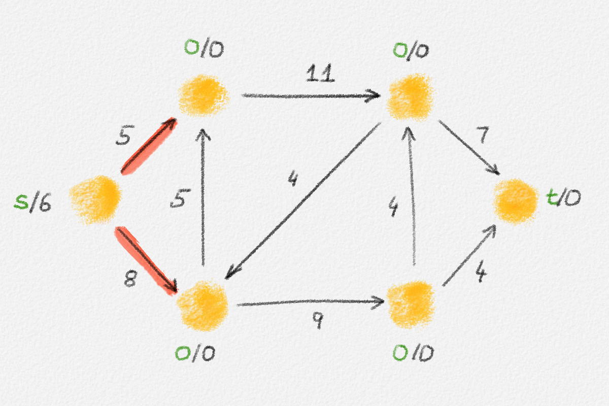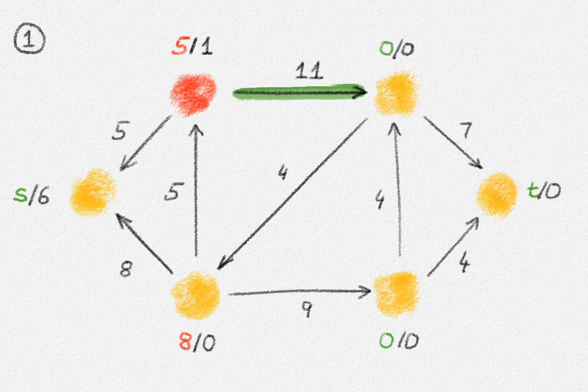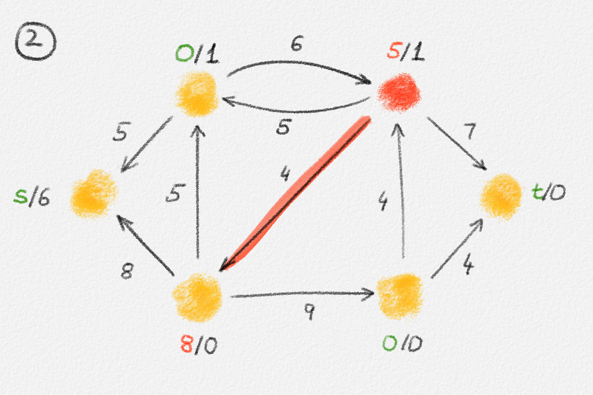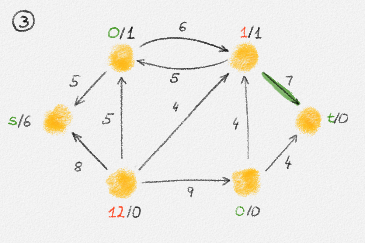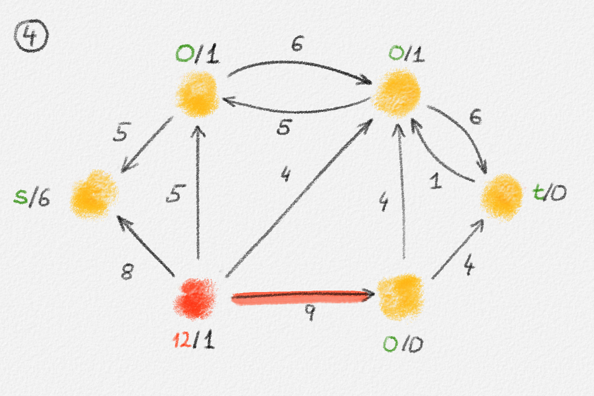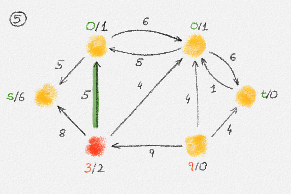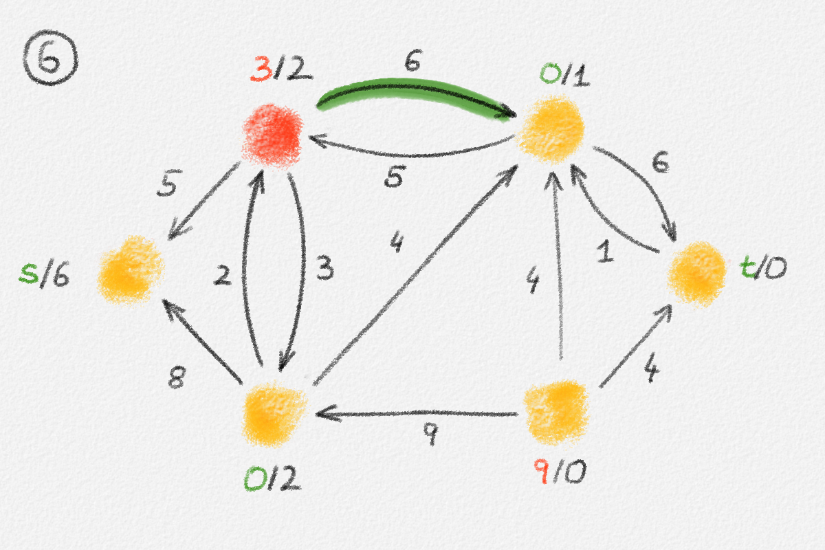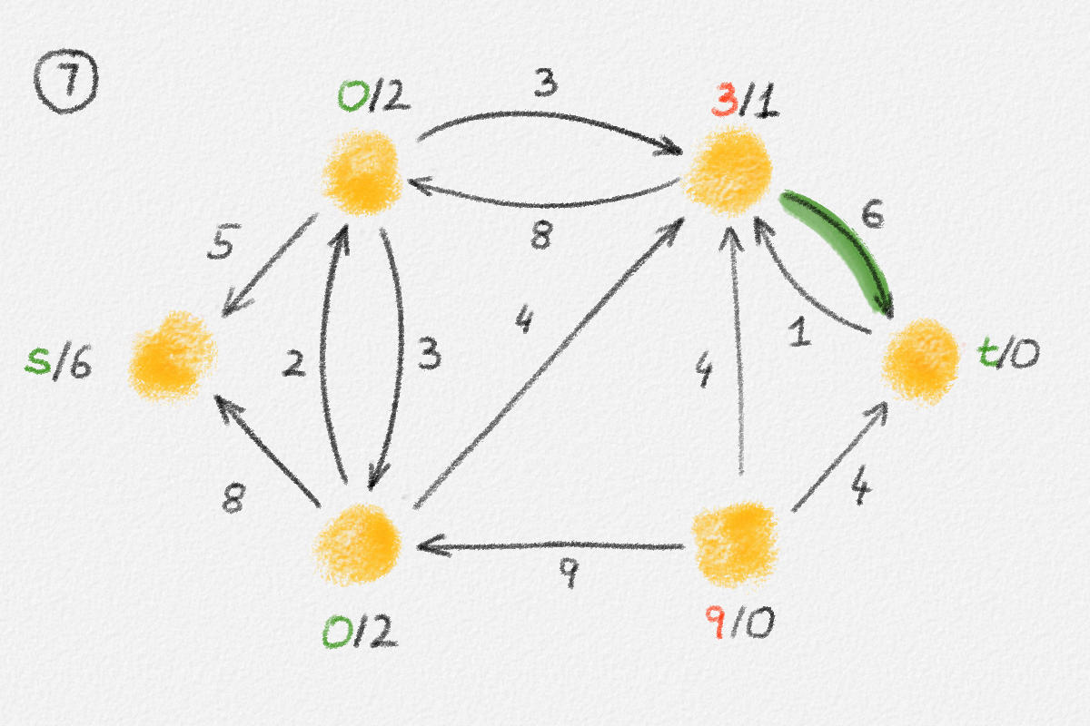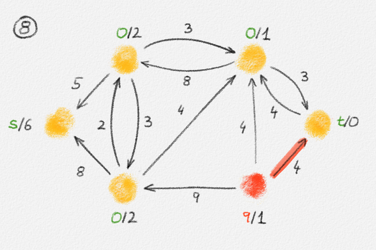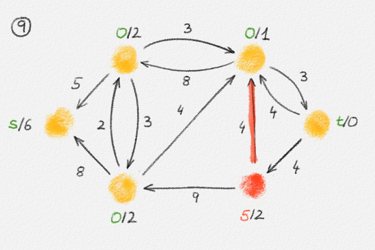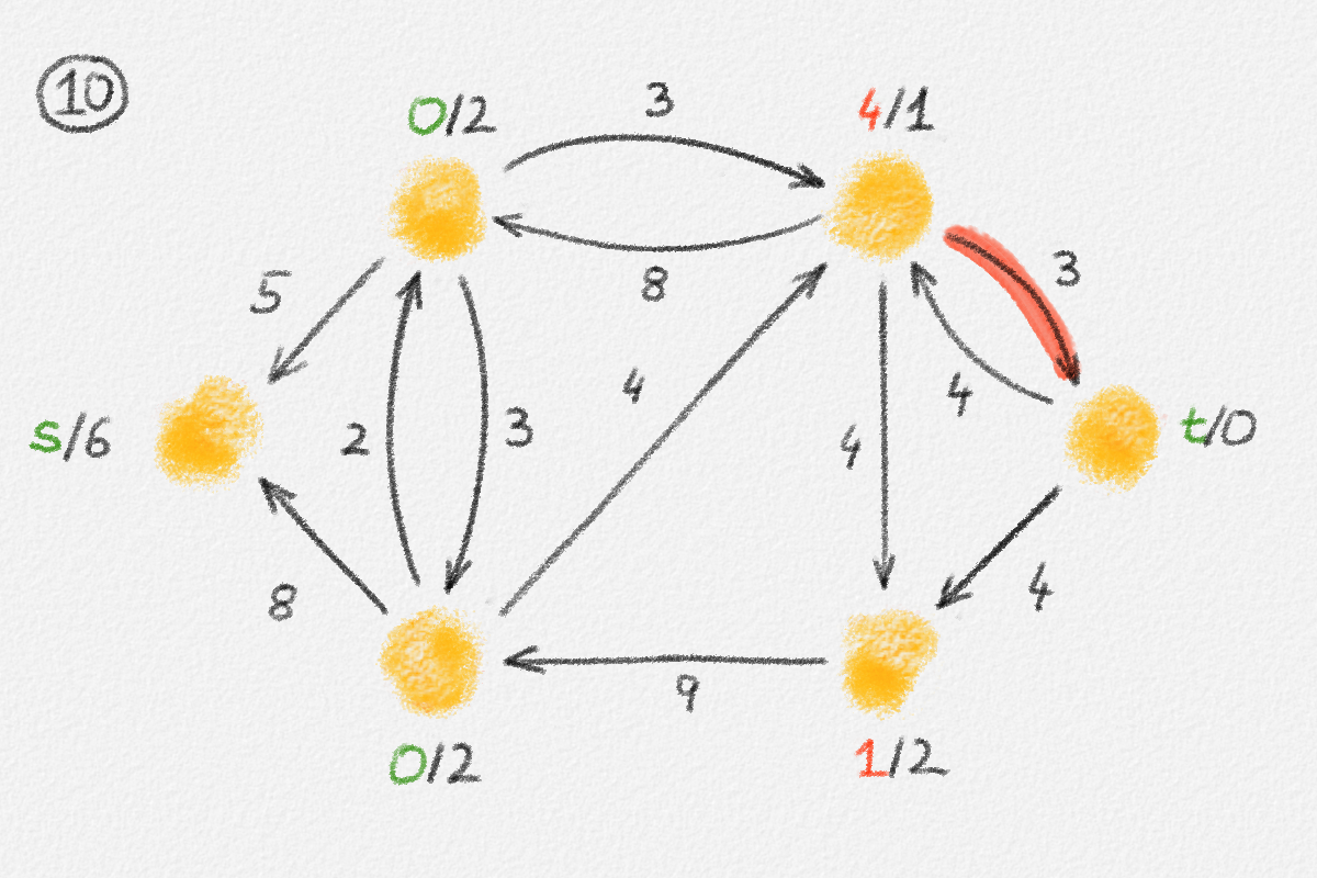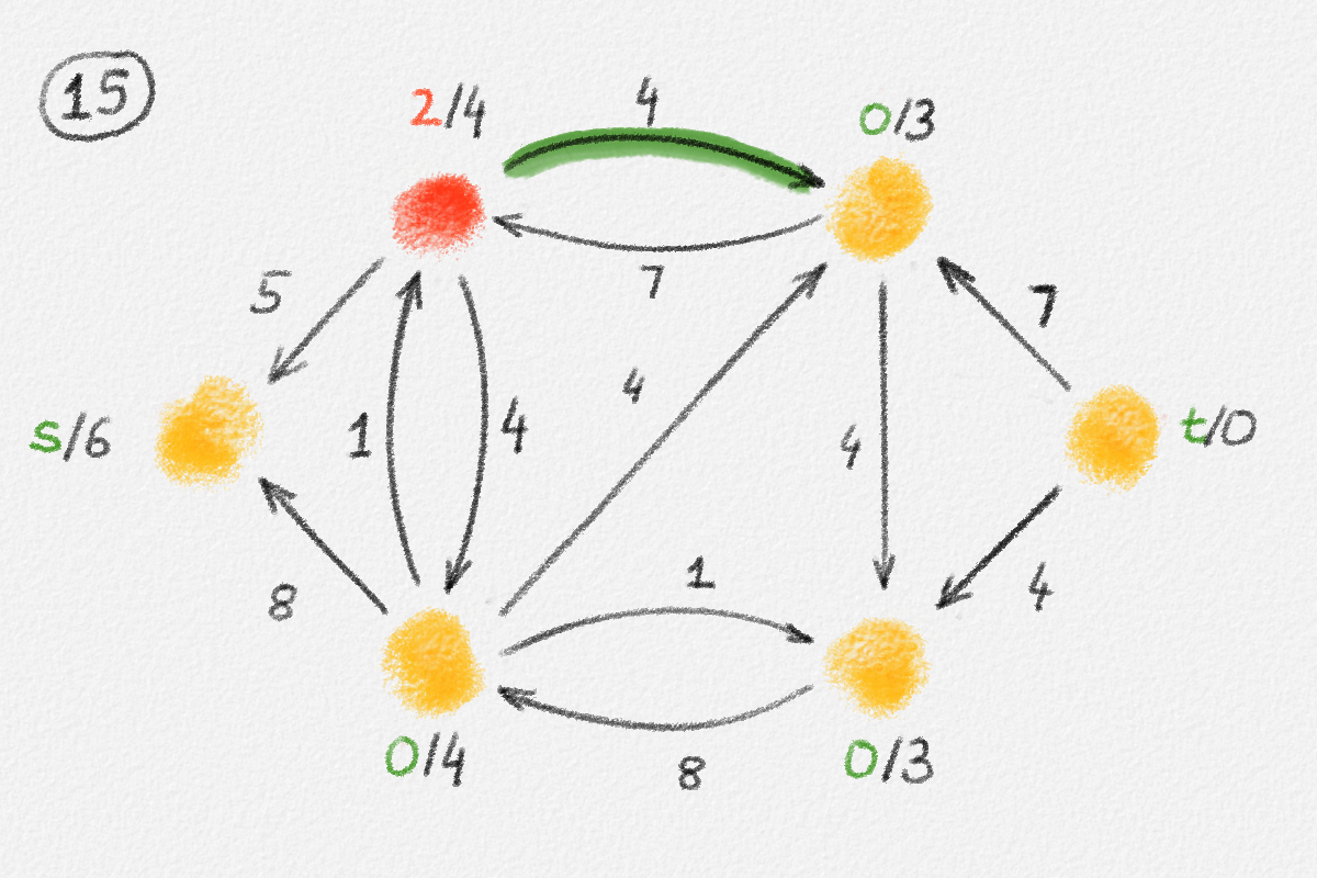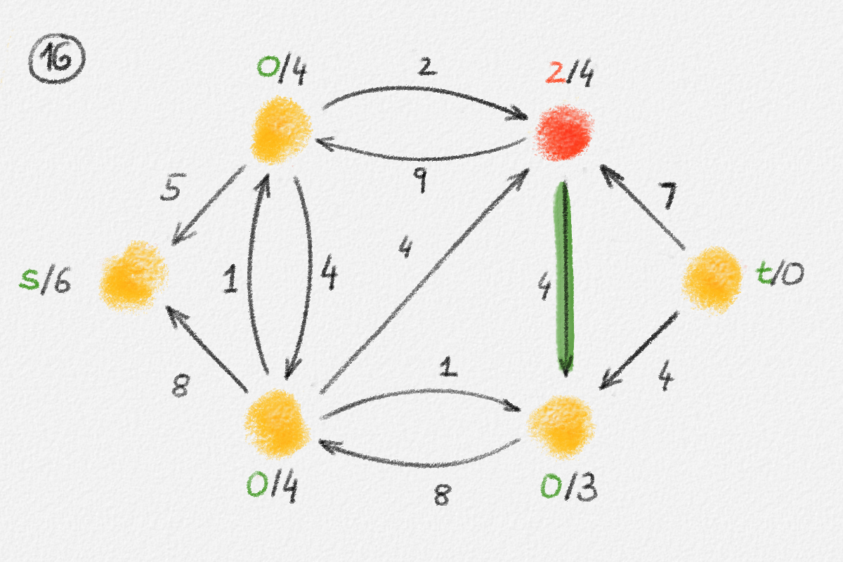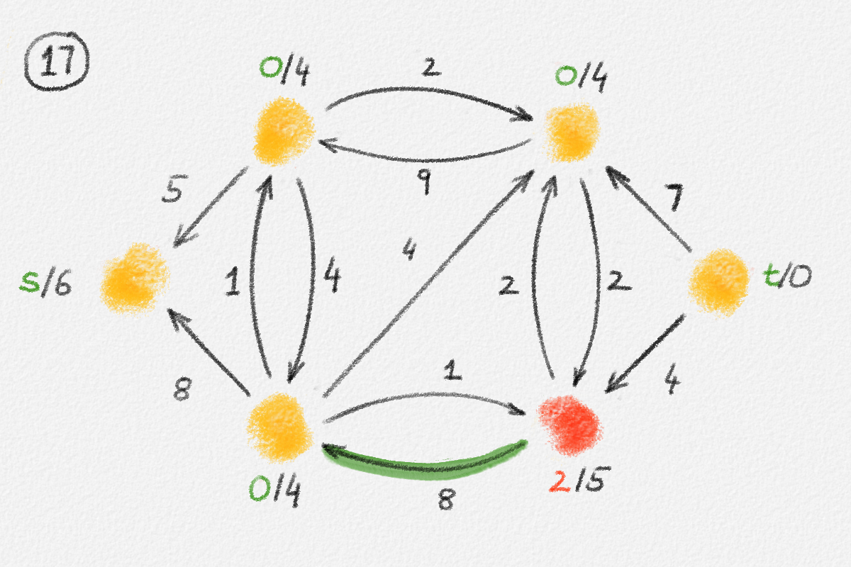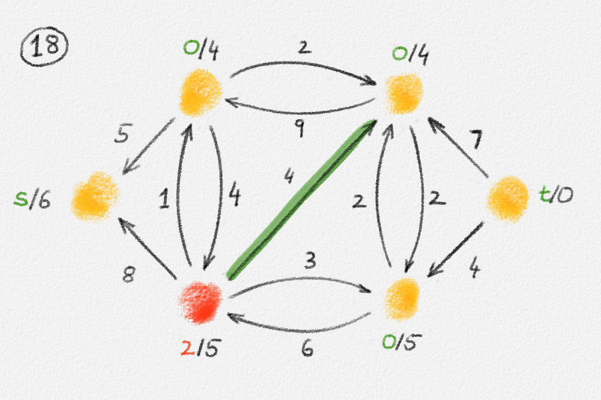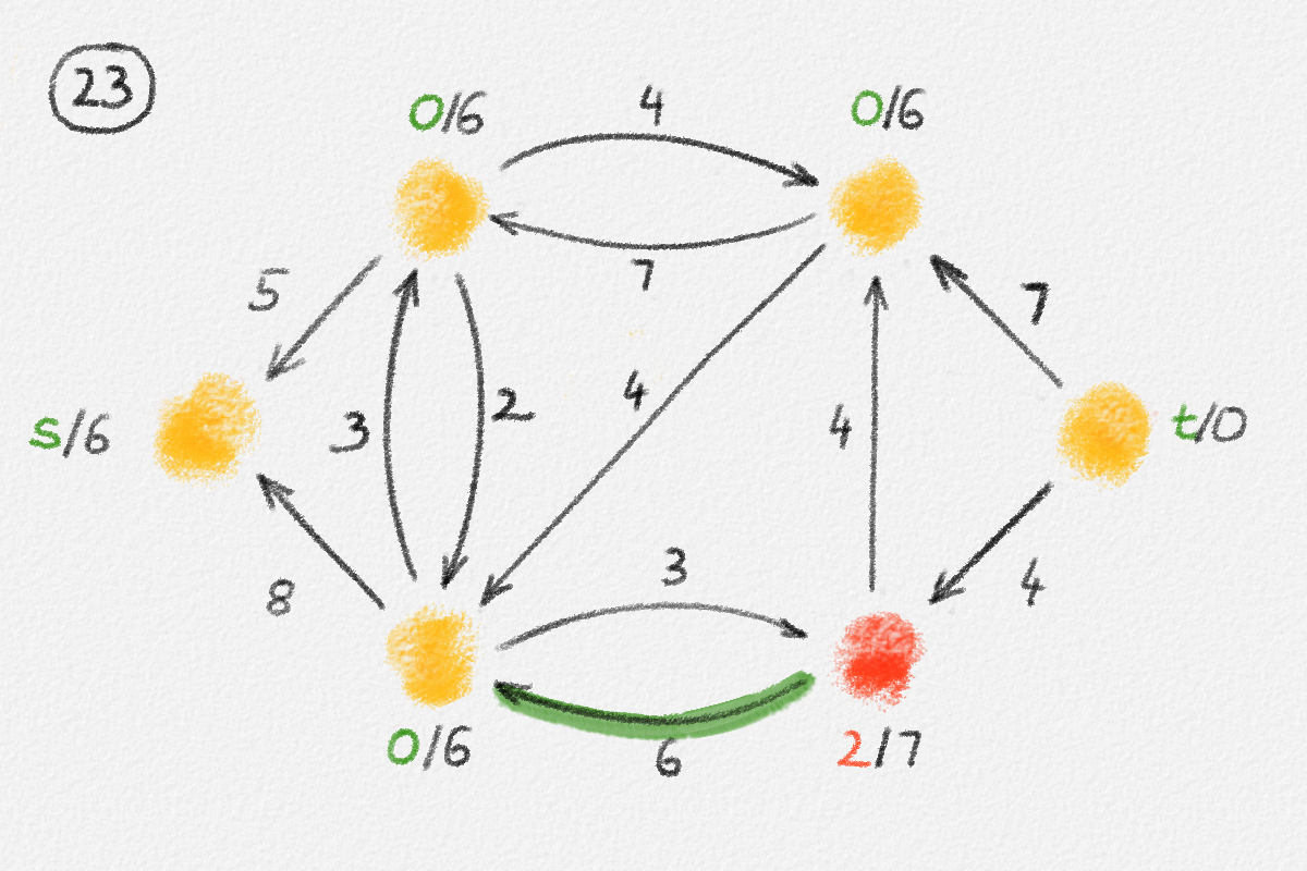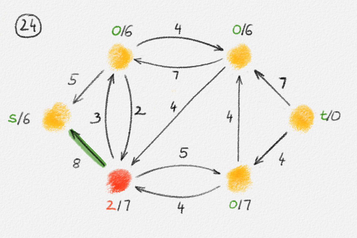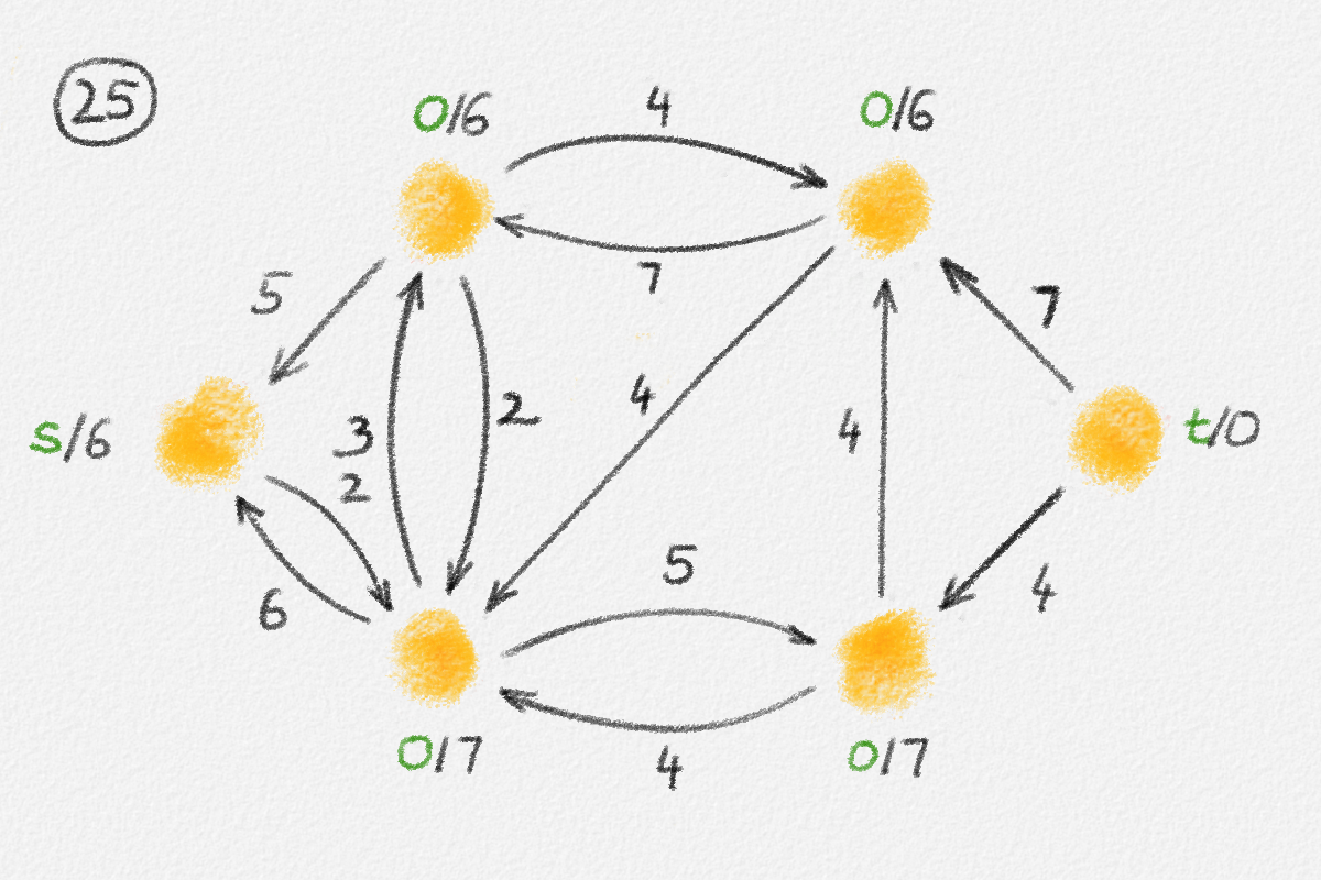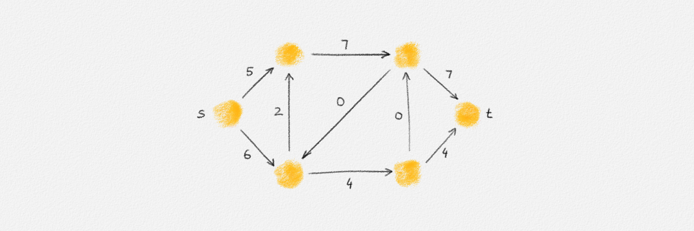Figure 5.16: Illustration of an application of the generic preflow-push algorithm to the network in Figure 5.1. The circled numbers indicate the iteration number. Only the residual network is shown. Edge labels are edge capacities. Black node labels are node heights. Coloured node labels are node excesses, shown in red if positive and in green if zero. \(s\) and \(t\) are labelled with their names instead, to make them recognizable; they never overflow. In each figure, the edge used to push flow to a neighbour is shown in red if it is a saturating push or in green if it is a non-saturating push. If the tail of the edge was relabelled to allow this push to happen, this tail node is shown in red. The final network in the bottom row shows the computed flow.

Termination: If there is no vertex \(x \notin \{s, t\}\) with positive excess, then \(f\) is a feasible \(st\)-flow. Exit the algorithm and return \(f\). We prove below that \(f\) is not only a feasible \(st\)-flow but a maximum \(st\)-flow at this point.

Push: If there exist an overflowing vertex \(x \notin \{s, t\}\) and an edge \((x,y) \in G^f\) with \(h_y = h_x - 1\), then push

\[\delta = \min\Bigl(e_x, u^f_{x,y}\Bigr)\]

units of flow "downhill" from \(x\) to \(y\). Formally, set

\[\begin{aligned} f_{y,x} &= f_{y,x} - \min\bigl(\delta, f_{y,x}\bigr)\\ f_{x,y} &= f_{x,y} + \max\bigl(0, \delta - f_{y,x}\bigr)\\ e_x &= e_x - \delta\\ e_y &= e_y + \delta. \end{aligned}\]

Clearly, this does not decrease \(e_y\) and does not make \(e_x\) negative. Similar to the analysis of augmenting path algorithms, it also maintains the capacity constraint for the edge \((x,y)\). Thus, \(f\) remains a valid preflow. The operation also maintains the validity of the height function \(h\):

Observation 5.11: After a Push operation, \(h\) remains a valid height function.

Proof: A Push operation does not change \(h_z\) for any vertex \(z \in V\). Thus, the validity of \(h\) can only be affected by changes in the edge set of \(G^f\). Pushing flow from \(x\) to \(y\) can only make \((x,y)\) disappear from \(G^f\) and \((y,x)\) appear in \(G^f\). The former cannot invalidate \(h\). The latter does not invalidate \(h\) because \(h_x = h_y + 1\), so \(h_y \le h_x + 1\). ▨

A Push operation is called saturating if \(u^f_{x,y} = 0\) after the Push operation, that is, if \(f_{y,x} = 0\) and \(f_{x,y} = u_{x,y}\). Otherwise, it is non-saturating.

The only reason why a non-saturating Push operation chooses not to push more flow from \(x\) to \(y\), in an attempt to make it saturating, is because \(e_x < u^f_{x,y}\). This gives the following observation:

Observation 5.12: After a non-saturating Push operation along an edge \((x,y)\), \(e_x = 0\).

Relabel: If no overflowing vertex \(x \notin \{s, t\}\) has an out-edge \((x,y)\) in \(G^f\) that satisfies \(h_y = h_x - 1\), then pick an overflowing vertex \(x \notin \{s, t\}\) and set

\[h_x = 1 + \min \bigl\{ h_y \mid (x,y) \in G^f \bigr\}.\]

Note that this value is well defined because \(e_x > 0\) means that some amount of flow enters \(x\) through some in-edge \((y,x) \in E\) and thus the edge \((x,y)\) is in \(G^f\).

Observation 5.13: Relabelling \(x\) increases \(h_x\).

Proof: Since \(x\) is being relabelled, every out-neighbour \(y\) of \(x\) in \(G^f\) satisfies \(h_y \ge h_x\). Thus, setting \(h_x = 1 + \min \bigl\{ h_y \mid (x,y) \in G^f \bigr\}\) increases \(h_x\) by at least one. ▨

Observation 5.14: After relabelling \(x\), \(h\) remains a valid height function.

Proof: Increasing \(h_x\) can only lead out-edges \((x,y)\) of \(x\) in \(G^f\) to violate the condition that \(h_x \le h_y + 1\). Since a relabel operation sets \(h_x = 1 + \min \bigl\{ h_y \mid (x,y) \in G^f \bigr\}\), none of \(x\)'s out-edges violates this condition. ▨

The following lemma states that, as long as \(f\) is not a feasible \(st\)-flow, either a Push or a Relabel operation is applicable. Thus, the behaviour of the algorithm is well defined.

Lemma 5.15: As long as \(f\) is not a feasible \(st\)-flow, either a Push or a Relabel operation is applicable.

Proof: If \(f\) is not a feasible \(st\)-flow, then there exists an overflowing vertex \(x \notin \{s, t\}\). As observed above, \(x\) has at least one out-neighbour in \(G^f\). If one of these out-neighbours, \(y\), satisfies \(h_x = h_y + 1\), then we can push flow from \(x\) to \(y\). Otherwise, \(x\) can be relabelled. ▨

To summarize the preflow-push algorithm so far: We initialize \(f\) so that all out-edges of \(s\) are saturated while any other edge \((x, y)\) satisfies \(f_{x,y} = 0\). The height function \(h\) sets \(h_s = n\) and \(h_x = 0\) for all \(x \ne s\). Then we repeatedly pick a vertex \(x \notin \{s, t\}\) with positive excess \(e_x\) and we either move some of this excess to an out-neighbour \(y\) of \(x\) in \(G^f\) with \(h_y = h_x - 1\) (a Push operation) or we increase \(x\)'s height to one more than the minimum height of \(x\)'s out-neighbours in \(G^f\) (a Relabel operation). Note that after a Relabel operation, \(x\) is able to push some of its excess to at least one of its out-neighbours because at least one out-neighbour \(y\) satisfies \(h_y = h_x - 1\) now. We keep applying Push and Relabel operations until every vertex \(x \notin \{s, t\}\) has excess \(0\). At this point, \(f\) is a feasible \(st\)-flow, which the algorithm returns.

Next we prove that the preflow-push algorithm, if it terminates, returns a maximum \(st\)-flow.

5.2.1.1. Correctness of the Generic Preflow-Push Algorithm

The next lemma will be crucial for showing that the preflow-push algorithm does indeed compute a maximum flow.

Lemma 5.16: At any point during the course of the preflow-push algorithm, there is no path from \(s\) to \(t\) in the residual network \(G^f\).

Proof: Assume for the sake of contradiction that the residual network \(G^f\) does contain a path \(P = \langle s=x_0, \ldots, x_k=t \rangle\) from \(s\) to \(t\) at some point during the course of the algorithm. We can assume w.l.o.g. that \(P\) is a simple path, that is, that it visits every vertex at most once. Thus, it has \(k \le n-1\) edges. By Observations 5.11 and 5.14, \(h\) is a valid height function at all times. Thus, \(P\) satisfies \[h_{x_{i-1}} \le h_{x_i} + 1 \quad \forall1 \le i \le k.\]

In particular,

\[n = h_s \le h_t + k \le h_t + n - 1 = n - 1,\]

a contradiction. ▨

The following theorem now establishes the correctness of the preflow-push algorithm under the assumption that the algorithm terminates:

Theorem 5.17: If the generic preflow-push algorithm terminates, then the edge labelling \(f\) it returns is a maximum \(st\)-flow.

Proof: At any point during the algorithm's execution, \(f\) is a valid preflow, that is, it satisfies all capacity constraints. Once the algorithm terminates, \(f\) also satisfies flow conservation. Thus, \(f\) is a feasible \(st\)-flow.

By Lemma 5.16, there is no path from \(s\) to \(t\) in \(G^f\). As shown in the proof of Theorem 5.4, this implies that \(f_s\) equals the capacity of some \(st\)-cut in \(G\) and is thus a maximum \(st\)-flow. ▨

5.2.1.2. Running Time Analysis of the Generic Preflow-Push Algorithm

It remains to show that the preflow-push algorithm always terminates, quickly. The following lemma will be used to bound the maximum height a node can have:

Lemma 5.18: If \(f\) is a preflow, then there exists a path in \(G^f\) from every overflowing vertex \(x\) to \(s\).

Proof: Let \(W\) be the set of vertices other than \(t\) reachable from \(x\) in \(G^f\) and assume for the sake of contradiction that \(s \notin W\). Since \(e_y \ge 0\) for all \(y \in W\) and \(e_x > 0\), we have

\begin{align} 0 &< \sum_{y \in W} e_z\\ &= \sum_{y \in W} \sum_{z \in V} \bigl(f_{z,y} - f_{y,z}\bigr)\\ &= \sum_{y \in W} \sum_{z \in W} \bigl(f_{z,y} - f_{y,z}\bigr) + \sum_{y \in W} \sum_{z \notin W} \bigl(f_{z,y} - f_{y,z}\bigr)\tag{5.9}\\ &= \sum_{y \in W} \sum_{z \notin W} \bigl(f_{z,y} - f_{y,z}\bigr)\tag{5.10}\\ &\le \sum_{y \in W} \sum_{z \notin W} f_{z,y}.\tag{5.11} \end{align}

(5.10) follows from (5.9) because the first sum in (5.9) counts every edge between vertices in \(W\) twice, once with positive sign and once with negative sign, so this sum is zero. (5.11) follows from (5.10) because \(f_{y,z} \ge 0\) for every edge \((y,z)\).

Now \(0 < \sum_{y \in W} \sum_{z \notin W} f_{z,y}\) implies that there exists an edge \((z, y)\) with \(z \notin W\), \(y \in W\), and \(f_{z,y} > 0\). Thus, \(G^f\) contains the edge \((y, z)\), a contradiction because \(y \in W\) and \(z \notin W\). ▨

Corollary 5.19: Every vertex \(x \in V \setminus \{ s, t \}\) satisfies \(h_x \le 2n - 1\).

Proof: Initially, every vertex \(x \in V \setminus \{ s, t \}\) satisfies \(h_x = 0\). The height of \(x\) changes only as a result of relabelling \(x\), which happens only when \(e_x > 0\). By Lemma 5.18, there exists a path \(P = \langle x = x_0, \ldots, x_k = s \rangle\) from \(x\) to \(s\) in \(G^f\) at this time. By Observations 5.11 and 5.14, \(h\) is a valid height function at all times. Thus, immediately after relabelling \(x\), we have \(h_{x_{i-1}} \le h_{x_i} + 1\) for all \(1 \le i \le k\). Since \(h_{x_k} = h_s = n\) and \(k \le n - 1\), this shows that \(h_x = h_{x_0} \le h_s + n - 1 = 2n - 1\). ▨

Corollary 5.19 provides the tool to bound the number of Relabel operations and the number of saturating Push operations the algorithm performs.

Lemma 5.20: The generic preflow-push algorithm performs at most \(2n(n-1)\) Relabel operations.

Proof: For every vertex \(x \in V \setminus \{ s, t \}\), \(h_x = 0\) initially and \(h_x \le 2n - 1\) at all times. By Observation 5.13, \(h_x\) increases every time \(x\) is relabelled. Thus, \(x\) is relabelled at most \(2n - 1\) times. By summing over all vertices in \(V \setminus \{ s, t \}\) (\(s\) and \(t\) are never relabelled), we obtain a bound of \((2n - 1)(n - 2) \le 2n(n-1)\) on the number of Relabel operations. ▨

Lemma 5.21: The generic preflow-push algorithm performs at most \(2nm\) saturating Push operations.

Proof: It suffices to prove that every edge \((x, y)\) is used for at most \(2n\) saturating Push operations, counting both Push operations from \(x\) to \(y\) and from \(y\) to \(x\). Since there are \(m\) edges, this shows that the total number of saturating Push operations is at most \(2nm\).

Consider a saturating Push operation from \(x\) to \(y\) and let \(\ell\) be the height of \(x\) at the time of this Push operation. Since the Push operation is saturating, we have \(u^f_{x,y} = 0\) after this Push operation. In order to push more flow from \(x\) to \(y\) after this Push operation, we need to increase \(u^f_{x,y}\) so it becomes positive again, which is possible only by pushing flow from \(y\) to \(x\).

At the time we push flow from \(y\) to \(x\), we must have \(\ell' = h_y = h_x + 1 \ge \ell + 1\), where the last inequality holds because, by Observation 5.13, vertex heights do not decrease over the course of the algorithm.

At the time of the next Push operation from \(x\) to \(y\), we must have \(h_x = h_y + 1 \ge \ell' + 1 \ge \ell + 2\), by the same argument. Thus, between any two saturating Push operations from \(x\) to \(y\), \(h_x\) increases by at least two.

Since \(h_x = 0\) initially and \(h_x \le 2n - 1\) at all times, this shows that we perform at most \(n\) saturating Push operations from \(x\) to \(y\). By an analogous argument, the number of saturating Push operations from \(y\) to \(x\) is also bounded by \(n\). Thus, at most \(2n\) saturating Push operations use the edge \((x, y)\), as claimed. ▨

The most difficult part of the analysis is bounding the number of non-saturating Push operations because an edge can be used for several non-saturating Push operations in the same direction without relabelling the endpoints.

Lemma 5.22: The generic preflow-push algorithm performs at most \(8n^2m\) non-saturating Push operations.

Proof: To prove this, we define a potential function

\[\Phi = \sum_{e_x > 0} h_x.\]

Initially, \(\Phi = 0\) because every vertex other than \(s\) has height zero and \(e_s = 0\). Moreover, since every vertex has a non-negative height, \(\Phi\) is never negative.

The proof idea now is to bound the increase in potential resulting from every Relabel and saturating Push operation and to show that every non-saturating Push operation decreases the potential by at least one. Specifically, we show that Relabel and saturating Push operations do not add more than \(8n^2m\) in total to the potential. Since every non-saturating Push operation decreases the potential by at least one and the potential is never negative, this shows that there are at most \(8n^2m\) non-saturating Push operations.

Relabel operations: A Relabel operation does not change the excess of any vertex and changes the height of a single vertex. Since \(h_x \ge 0\) before the Relabel operation and \(h_x \le 2n - 1\) after the Relabel operation, this increases \(\Phi\) by at most \(2n - 1\).

Saturating Push operations: A saturating Push operation along an edge \((x, y)\) does not alter the height of any vertex, may or may not reduce \(x\)'s excess to \(0\), and results in \(y\) having positive excess after the Push operation. Thus, the greatest increase in potential is achieved if \(e_x > 0\) before and after the Push operation—so \(x\)'s contribution to \(\Phi\) does not change—and \(e_y = 0\) before the Push operation and \(e_y > 0\) after the Push operation—so \(y\)'s contribution to \(\Phi\) increases by \(h_y\). Since \(h_y \le 2n - 1\), this shows that a saturating Push operation increases \(\Phi\) by at most \(2n - 1\).

Total increase in potential: By Lemmas 5.20 and 5.21, the total number of Relabel and saturating Push operations is at most \(2n(n-1) + 2nm \le 4nm\) because we can assume that \(G\) is connected and, hence, \(m \ge n - 1\). As just observed, each such operation increases \(\Phi\) by at most \(2n - 1\). Thus, the total increase in potential due to Relabel and saturating Push operations is less than \(8n^2 m\).

Non-saturating Push operations: A non-saturating Push operation along an edge \((x, y)\) does not alter the height of any vertex, decreases \(e_x\) from \(e_x > 0\) to \(e_x = 0\) and may change \(e_y\) from \(e_y = 0\) to \(e_y > 0\). Thus, the decrease in potential is at least \(h_x - h_y\).

Since we push flow from \((x, y)\), we have \(h_x = h_y + 1\) at the time of the Push operation. Thus, \(\Phi\) decreases by at least one.

Since Relabel and saturating Push operations increase the potential by at most \(8n^2 m\) and every non-saturating Push operation decreases the potential by at least one, we obtain a bound of \(8n^2 m\) on the total number of non-saturating Push operations. ▨

Theorem 5.23: The generic preflow-push algorithm runs in \(O\bigl(n^2m\bigr)\) time.

Proof: By Lemmas 5.20, 5.21, and 5.22, the preflow-push algorithm performs \(O\bigl(n^2\bigr)\) Relabel and \(O\bigl(n^2m\bigr)\) Push operations. The following exercise asks you to show how to implement every Relabel operation in \(O(n)\) time and every Push operation in constant time, and to show how to implement a data structure that can be used to pick the next vertex to be relabelled or the next edge along which to push flow in constant time. Thus, the total cost of the algorithm is \(O\bigl(n^2 \cdot n + n^2m\bigr) = O\bigl(n^2m\bigr)\). ▨

Exercise 5.2:

• Prove that every Relabel operation can be implemented in \(O(n)\) time and that every Push operation can be implemented in \(O(1)\) time.

• Provide a data structure that supports a NextOp operation, which returns either an edge \((x, y)\) that can be used for a Push operation (i.e., \(e_x > 0\), \(u^f_{x,y} > 0\), and \(h_x = h_y + 1\)) or a vertex \(x\) with \(e_x > 0\) to be relabelled if no such edge \((x, y)\) exists.

  • This NextOp operation should take constant time.
  • Updating the data structure after a Relabel operation should take \(O(n)\) time.
  • Updating it after a Push operation should take constant time.

5.2.2. The Relabel-To-Front Algorithm*

One characteristic of the generic preflow-push algorithm is that it delays Relabel operations for as long as possible: As long as there exists an overflowing vertex \(x\) with an admissible out-edge \((x, y)\), it prefers to push flow from \(x\) to \(y\) along this edge over relabelling a vertex.

We call an edge \((x, y)\) admissible if \(u^f_{x,y} > 0\) and \(h_x = h_y + 1\), that is, if we can push flow along this edge.

This is a natural strategy because the main goal of the algorithm is to push flow along edges, not to relabel vertices. In addition, as discussed in Exercise 5.2, Push operations are cheaper than Relabel operations. Nevertheless, it turns out that once we decide to reduce the excess at some vertex \(x\) by pushing flow from \(x\) to its neighbours, it is beneficial to completely eliminate \(x\)'s excess, if necessary by relabelling \(x\) even though there may still exist admissible edges elsewhere in the graph. This idea leads to the relabel-to-front algorithm, which achieves a running time of \(O\bigl(n^3\bigr)\). The relabel-to-front algorithm is a variant of the generic preflow-push algorithm: It simply chooses the order in which to perform Push and Relabel operations more carefully (and chooses the right data structures to maintain its state). Thus, it is a correct maximum flow algorithm.

Note that the generic preflow-push algorithm almost achieves an \(O\bigl(n^3\bigr)\) running time already. The only reason its running time may be as high as \(O\bigl(n^2m\bigr)\) is because this is the number of non-saturating Push operations it may perform. The goal of the relabel-to-front algorithm is thus to reduce the number of these operations to \(O\bigl(n^3\bigr)\).

5.2.2.1. The Discharge Operation

The heart of the relabel-to-front algorithm is the following Discharge operation, which takes a single vertex \(x\) as its argument and ensures that \(e_x = 0\) at the time this operation returns. This procedure relies on a linked list \(\textrm{NBR}(x)\) and a pointer \(\textrm{CUR}(x)\) into this list. \(\textrm{NBR}(x)\) stores all neighbours of \(x\), that is, all vertices \(y\) such that \\(x,y)\) or \((y,x)\) is an edge of \(G\). The elements in this list are not stored in any particular order. \(\textrm{CUR}(x)\) is the next neighbour to which the operation tries to push excess flow from \(x\) if the edge \((x,y)\) is admissible.

PROCEDURE \(\boldsymbol{\textbf{Discharge}(G, u, f, h, x)}\):

---

INPUT:

• A directed graph \(G = (V, E)\)
• A capacity labelinng \(u : E \rightarrow \mathbb{R}^+\) of its edges
• A preflow \(f : E \rightarrow \mathbb{R}^+\)
• A height function \(h : V \rightarrow [0, 2n - 1]\)
• A vertex \(x \in V\)

OUTPUT:

• An updated preflow \(f' : E \rightarrow \mathbb{R}^+\) such that \(x\)'s excess \(e_x = 0\)
• An updated height function \(h' : V \rightarrow [0, 2n - 1]\)

---

1.     WHILE \(e_x > 0\) DO
2.         IF \(\textrm{CUR}(x) = \textrm{NULL}\) THEN
3.             \(\textrm{Relabel}(G, f, h, x)\)
4.             \(\textrm{CUR}(x) = \textrm{HEAD}(\textrm{NBR}(x))\)
5.         ELSIF the edge \((x, \textrm{CUR}(x))\) is admissible THEN
6.             \(\textrm{Push}(G, f, (x, \textrm{CUR}(x)))\)
7.         ELSE
8.             \(\textrm{CUR}(x) = \textrm{NEXT}(\textrm{CUR}(x))\)
9.     RETURN \((f, h)\)

The while-loop relabels \(x\) and pushes flow from \(x\) to its neighbours until \(x\)'s excess is zero.

Lines 5–8 hold no mystery: As long as \(e_x > 0\) and the current edge \((x, \textrm{CUR}(x))\) is admissible, the algorithm pushes excess from \(x\) to \(\textrm{CUR}(x)\) along this edge. If \((x, \textrm{CUR}(x))\) is not admissible, line 8 advances \(\textrm{CUR}(x)\) to the next neighbour \(y\) in the hope that the edge \((x, y)\) is admissible.

A more interesting aspect of the Discharge operation is that it relabels \(x\) and then resets \(\textrm{CUR}(x)\) to point to the head of \(\textrm{NBR}(x)\) if \(\textrm{CUR}(x) = \textrm{NULL}\), that is, once it has reached the end of the list of \(x\)'s neighbours. Since a Relabel operation is applicable only if none of x's out-edges is admissible, we need to prove that indeed \(x\) has no admissible out-edges once \(\textrm{CUR}(x) = \textrm{NULL}\). This follows immediately from the following invariant:

Invariant 5.24: There is no neighbour \(y\) of \(x\) that precedes \(\textrm{CUR}(x)\) in \(\textrm{NBR}(x)\) and such that the edge \((x, y)\) is admissible.

Proof: Initially, \(\textrm{CUR}(x) = \textrm{HEAD}(\textrm{NBR}(x))\), so the invariant holds. The invariant may be violated by changing \(\textrm{CUR}(x)\) or by creating admissible edges. First we prove that changing \(\textrm{CUR}(x)\) does not invalidate the invariant.

When we advance \(\textrm{CUR}(x)\) from some vertex \(y\) to its successor \(z \in \textrm{NBR}(x)\), then \(\textrm{CUR}(x)\) has the same predecessors in \(\textrm{NBR}(x)\) as before, plus \(y\). By the invariant, the edge \((x, w)\) is inadmissible for every predecessor \(w\) of \(y\) in \(\textrm{NBR}(x)\). Since advancing \(\textrm{CUR}(x)\) from \(y\) to \(z\) does not create any admissible edges, these edges remain inadmissible. The edge \((x, y)\) is inadmissible because this is the condition for advancing \(\textrm{CUR}(x)\) from \(y\) to \(z\) in line 8 of the Discharge procedure. Thus, the invariant continues to hold.

After setting \(\textrm{CUR}(x) = \textrm{HEAD}(\textrm{NBR}(x))\) in line 4 of the Discharge procedure, \(\textrm{CUR}(x)\) has no predecessors in \(\textrm{NBR}(x)\), so this cannot invalidate the invariant either.

Next consider the creation of admissible edges using Push Relabel operations.

By Lemma 5.25 below, a Push operation does not create any admissible edges. Thus, every edge \((x, w)\) such that \(w\) precedes \(\textrm{CUR}(x)\) in \(\textrm{NBR}(x)\) remains inadmissible after a Push operation.

By Lemma 5.26 below, all edges that become admissible as a result of a \(\boldsymbol{\textbf{Relabel}(w)}\) operation are out-edges of \(w\). Thus, if \(w \ne x\), all edges \((x, v)\) such that \(v\) precedes \(\textrm{CUR}(x)\) in \(\textrm{NBR}(x)\) remain inadmissible after any \(\boldsymbol{\textbf{Relabel}(w)}\) operation with \(w \ne x\).

A \(\boldsymbol{\textbf{Relabel}(x)}\) operation may create admissible out-edges of \(x\), but the only place in algorithm where this operation is called is in line 3 of a \(\boldsymbol{\textbf{Discharge}(x)}\) operation; line 4 then sets \(\textrm{CUR}(x) = \textrm{HEAD}(\textrm{NBR}(x))\), so there is no neighbour \(v\) of \(x\) that precedes \(\textrm{CUR}(x)\) in \(\textrm{NBR}(x)\) at all.

As we will see shortly, the relabel-to-front algorithm makes no changes to \(\textrm{CUR}(x)\), the preflow or the height function outside the Discharge procedure. Thus, the invariant is maintained at all times. ▨

Lemma 5.25: A Push operation does not create any admissible edges.

Proof: Consider an edge \((x, y)\) that is inadmissible, which means that \(h_x \ne h_y + 1\) or \(u^f_{x,y} = 0\).

A \(\boldsymbol{\textbf{Push}(w, z)}\) operation does not alter the height function \(h\). Thus, if \((x, y)\) is inadmissible because \(h_x \ne h_y + 1\), it remains inadmissible after the \(\textbf{Push}(w, z)\) operation.

If \(u^f_{x,y} = 0\) before the \(\boldsymbol{\textbf{Push}(w, z)}\) operation, then the edge remains inadmissible after the \(\boldsymbol{\textbf{Push}(w, z)}\) operation unless \(u^f_{x,y} > 0\) after the Push operation. This is possible only if \(x = z\) and \(y = w\) because \(u^f_{w,z}\) decreases as a result of a \(\boldsymbol{\textbf{Push}(w, z)}\) operation, \(u^f_{z,w}\) increases as a result of such an operation, and all other residual capacities remain unchanged. However, since we call \(\boldsymbol{\textbf{Push}(w, z)}\) only if the edge \((w, z)\) is admissible, that is, if \(h_w = h_z + 1\), this implies that \(h_x = h_y - 1\), that is, the edge \((x, y)\) remains inadmissible even if \(u^f_{x,y} > 0\) after the \(\boldsymbol{\textbf{Push}(w,z)}\) operation. ▨

Lemma 5.26: If an edge \((x, y)\) becomes admissible as a result of a \(\boldsymbol{\textbf{Relabel}(z)}\) operation, then \(x = z\). Moreover, \(z\) has no admissible in-edges after a \(\boldsymbol{\textbf{Relabel}(z)}\) operation.

Proof: Consider an edge \((x, y)\) that is inadmissible and such that \(x \ne z\). This means that \(h_x \ne h_y + 1\) or \(u^f_{x,y} = 0\). A \(\boldsymbol{\textbf{Relabel}(z)}\) operation does not alter the flow function \(f\) and thus neither the residual capacities of the edges. Thus, if \(u^f_{x,y} = 0\) before a \(\boldsymbol{\textbf{Relabel}(z)}\) operation, then \(u^f_{x,y} = 0\) after it, and the edge \((x, y)\) remains inadmissible.

If \(u^f_{x,y} > 0\), then \(h_x \ne h_y + 1\) before the Relabel operation. If \(y \ne z\), \(\boldsymbol{\textbf{Relabel}(z)}\) does not change \(h_x\) or \(h_y\) because we assumed above that \(x \ne z\), so the edge \((x, z)\) remains inadmissible.

If \(y = z\), then observe that before the \(\boldsymbol{\textbf{Relabel}(z)}\) operation, \(h_x \le h_y + 1\). This follows because the algorithm starts with a valid height function and Observations 5.11 and 5.14 show that Push and Relabel operations don't invalidate the height function. By Observation 5.13, a \(\boldsymbol{\textbf{Relabel}(z)}\) operation increases \(h_z = h_y\). Thus, \(h_x \le h_y\) after the \(\boldsymbol{\textbf{Relabel}(z)}\) operation, that is, the edge \((x, y)\) remains inadmissible. This finishes the proof that any inadmissible edge \((x,y)\) remains inadmissible after a \(\boldsymbol{\textrm{Relabel}(z)}\) operation unless \(x = z\).

Finally, consider an in-edge \((x, z)\) of \(z\). If this edge is admissible after relabelling \(z\), then \(h_x = h_z + 1\) after the \(\boldsymbol{\textbf{Relabel}(z)}\) operation and \(u^f_{x,z} > 0\) before and after the operation. By Observation 5.13, \(h_z\) increases as a result of relabelling \(z\). Thus, \(h_x > h_z + 1\) before the \(\boldsymbol{\textbf{Relabel}(z)}\) operation. By Observations 5.11 and 5.14, however, \(h\) is a valid height function at all times, that is, there exists no edge \((x,z)\) with \(u^f_{x,z} > 0\) and \(h_x > h_z + 1\) at any time during the algorithm. Thus, \(z\) has no admissible in-edge after relabelling \(z\). ▨

We have shown that Discharge operations apply Push and Relabel operations only when they are applicable. As we will see next, the relabel-to-front algorithm updates the flow and height function only via Discharge operations. Thus, it maintains a valid preflow and a valid height function.

5.2.2.2. The Algorithm

The relabel-to-front algorithm (procedure RelabelToFront below) derives its name from the manner in which it maintains the list of vertices to be discharged. An illustration of this algorithm is given in Figure 5.17.

PROCEDURE \(\boldsymbol{\textbf{RelabelToFront}(G, u, s, t)}\):

---

INPUT:

• A directed graph \(G = (V, E)\)
• A capacity labeling \(u : E \rightarrow \mathbb{R}^+\) of its edges
• A source vertex \(s\)
• A sink vertex \(t\)

OUTPUT:

• A maximum \(st\)-flow \(f : E \rightarrow \mathbb{R}^+\)

---

1.     FOR every vertex \(x \in V\) DO
2.         \(h_x = 0\)
3.     \(h_s = n\)
4.     FOR every edge \(e \in E\) DO
5.         \(f_e = 0\)
6.     FOR every out-neighbour \(y\) of \(s\) in \(G\) DO
7.         \(f_{s,y} = u_{s,y}\)
8.     \(L = V\)
9.     \(x = \textrm{HEAD}(L)\)
10.     WHILE \(x \ne \textrm{NULL}\) DO
11.         \(h_x' = h_x\)
12.         \((f, h) = \textbf{Discharge}(G, u, f, h, x)\)
13.         IF \(h_x > h_x'\) THEN
14.             Move \(x\) to the front of \(L\)
15.         \(x = \textrm{NEXT}(x)\)
16.     RETURN \(f\)

The algorithm maintains the vertices of \(G\) in a doubly-linked list \(L\), initially stored in no particular order, and initializes \(x\) to be the first vertex in \(L\). Then, as long as \(x \ne \textrm{NULL}\), it calls \(\boldsymbol{\textbf{Discharge}(x)}\) to ensure that \(x\)'s excess is zero and then advances \(x\) to the next vertex in \(L\). If \(\boldsymbol{\textbf{Discharge}(x)}\) relabels \(x\), which can be detected by observing an increase in \(x\)'s height \(h_x\), then the algorithm moves \(x\) to the front of the list \(L\) before advancing to \(x\)'s successor, that is, the new current vertex \(x\) after the current operation is the second vertex in \(L\) even if \(x\) was fairly close to the end of \(L\) before the \(\boldsymbol{\textbf{Discharge}(x)}\) operation. Thus, the algorithm may iterate over the vertices in \(L\) several times. Can this process continue forever or will the algorithm eventually reach a state when \(x \ne \textrm{NULL}\), so the algorithm terminates? This is the question we answer in the next section.

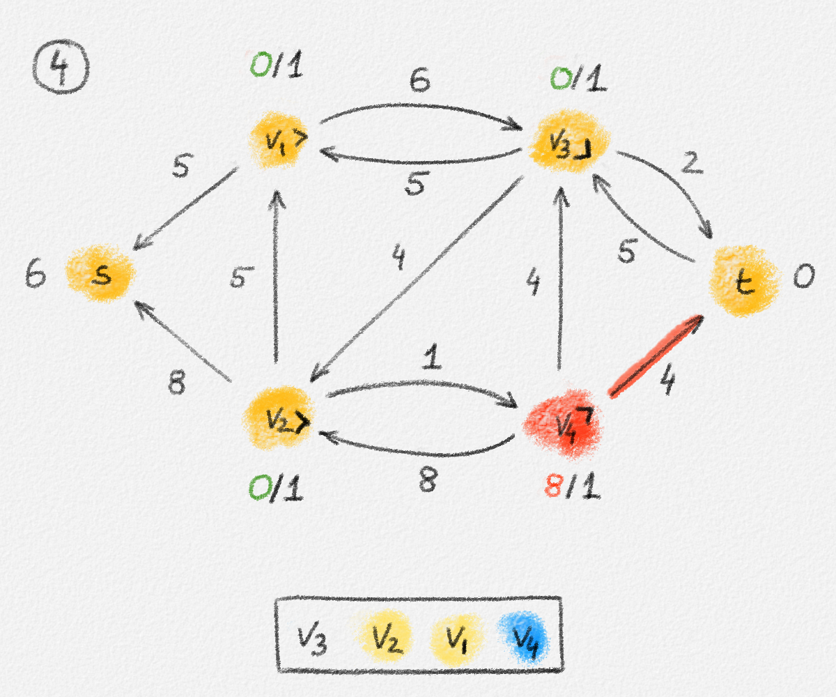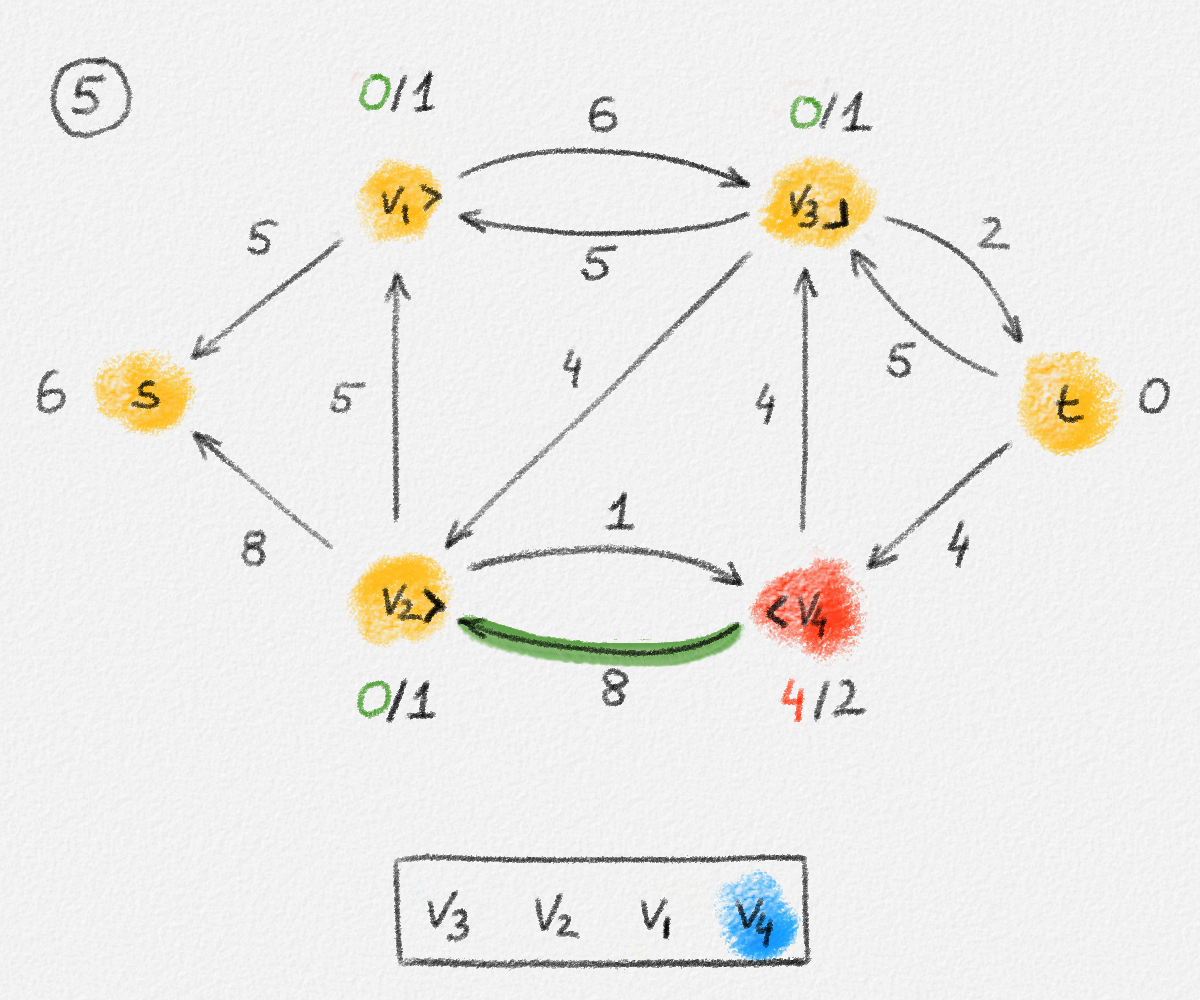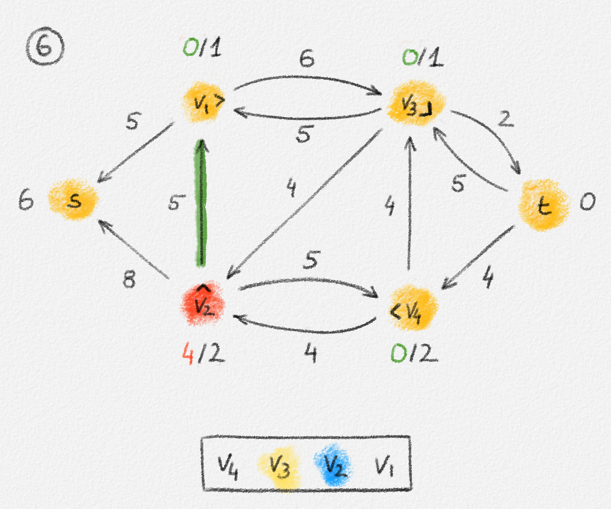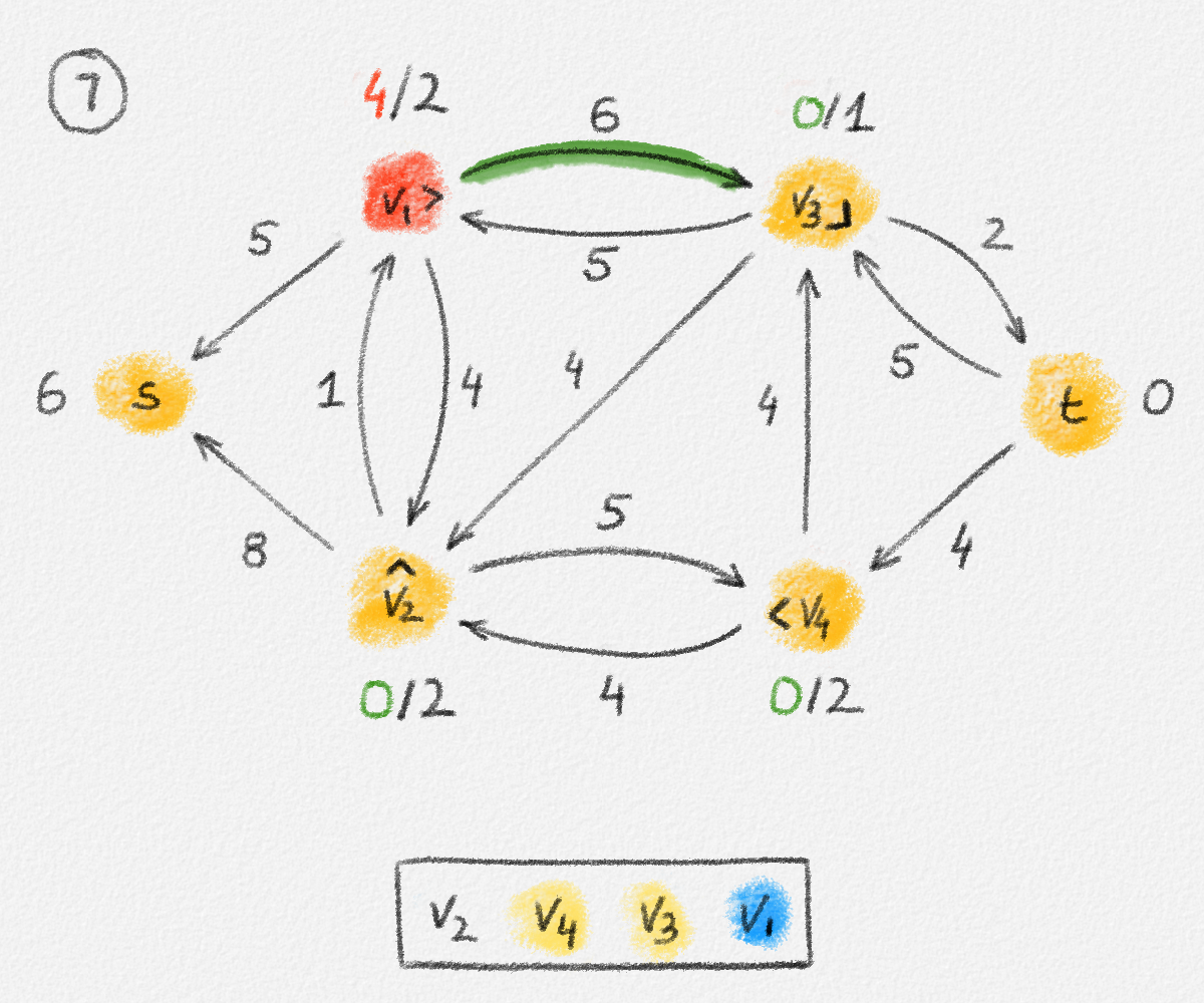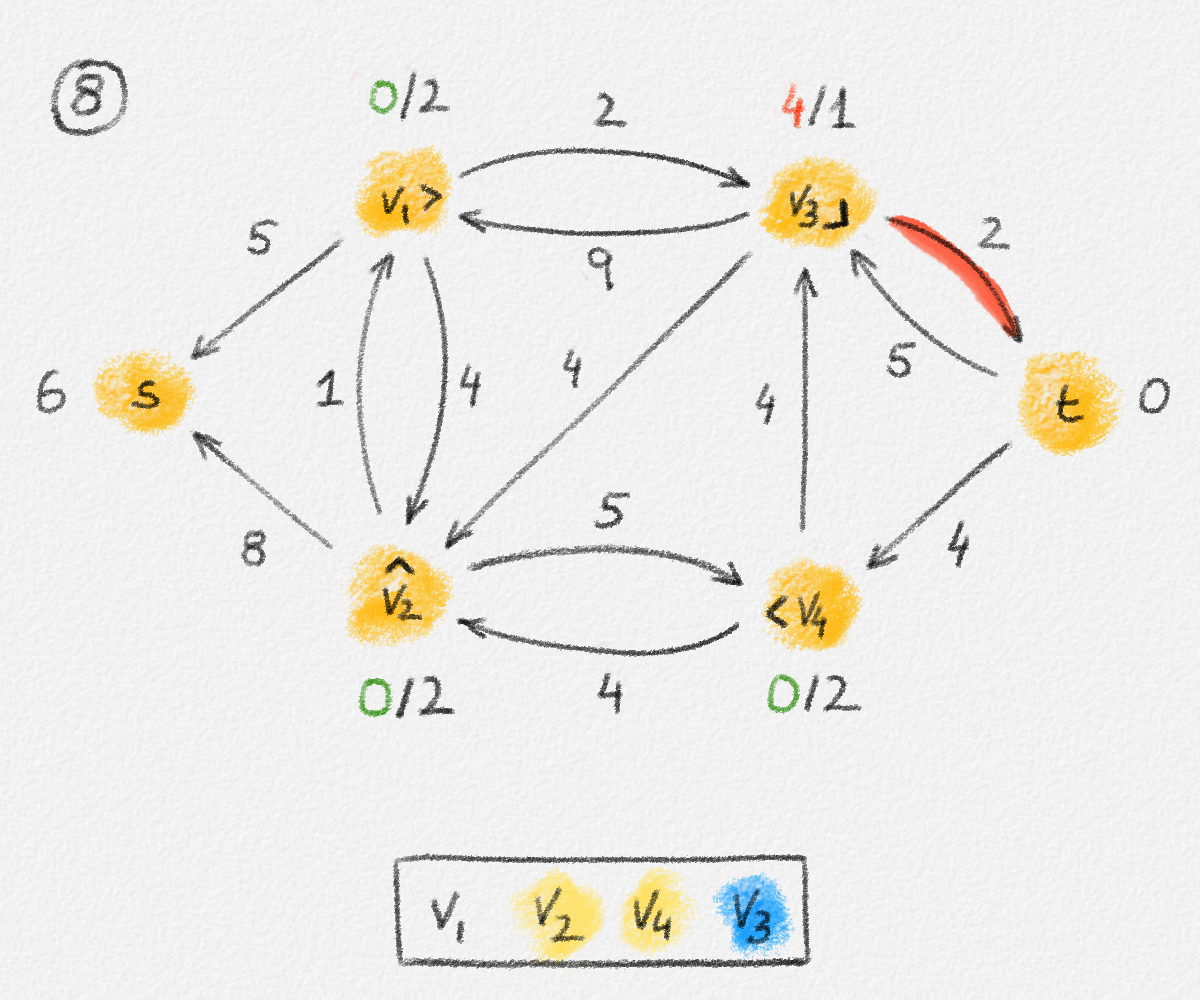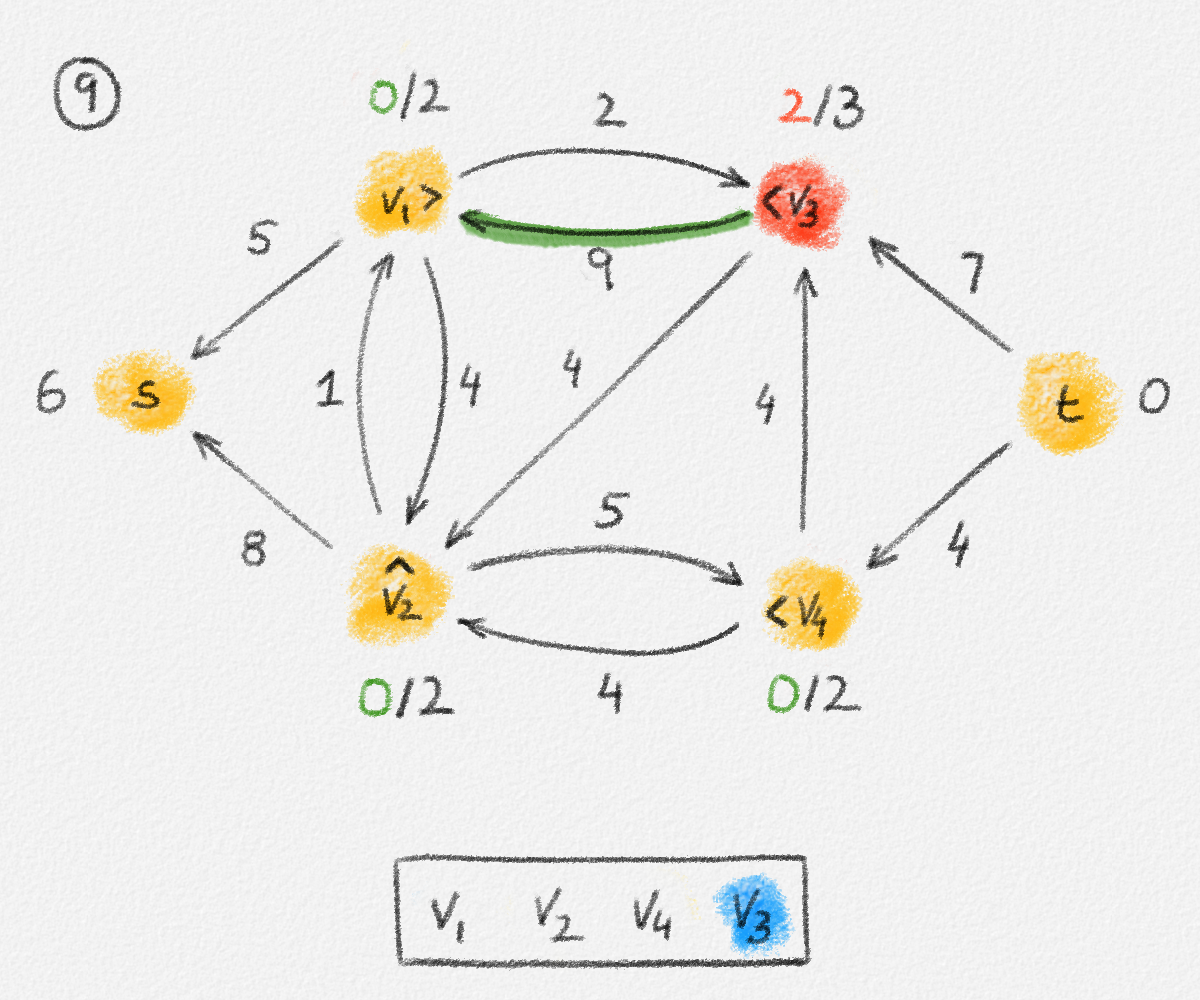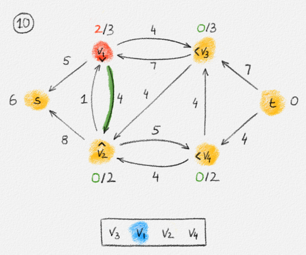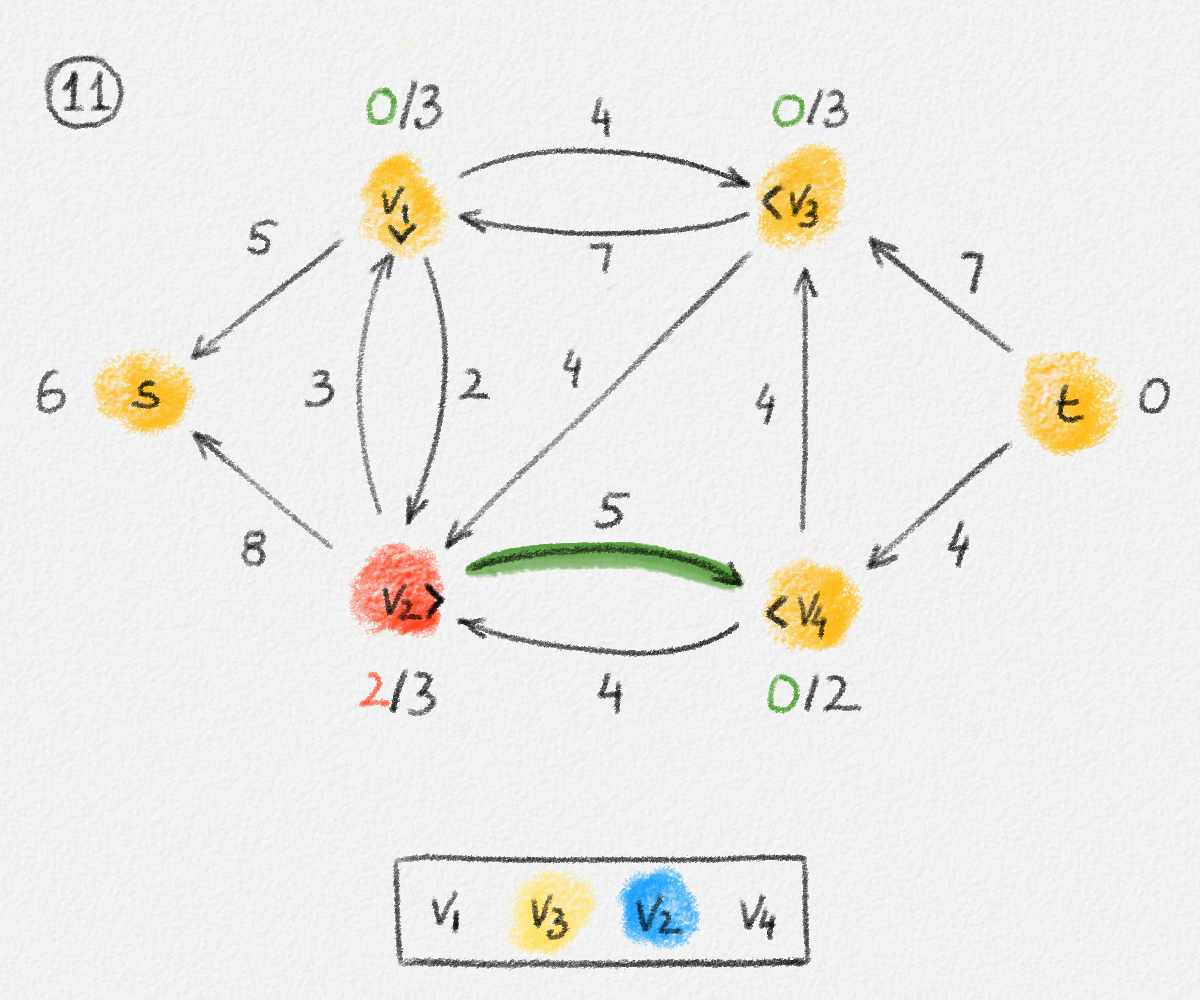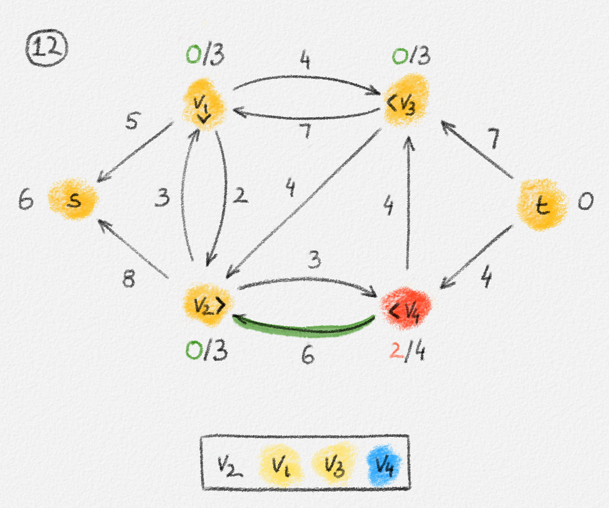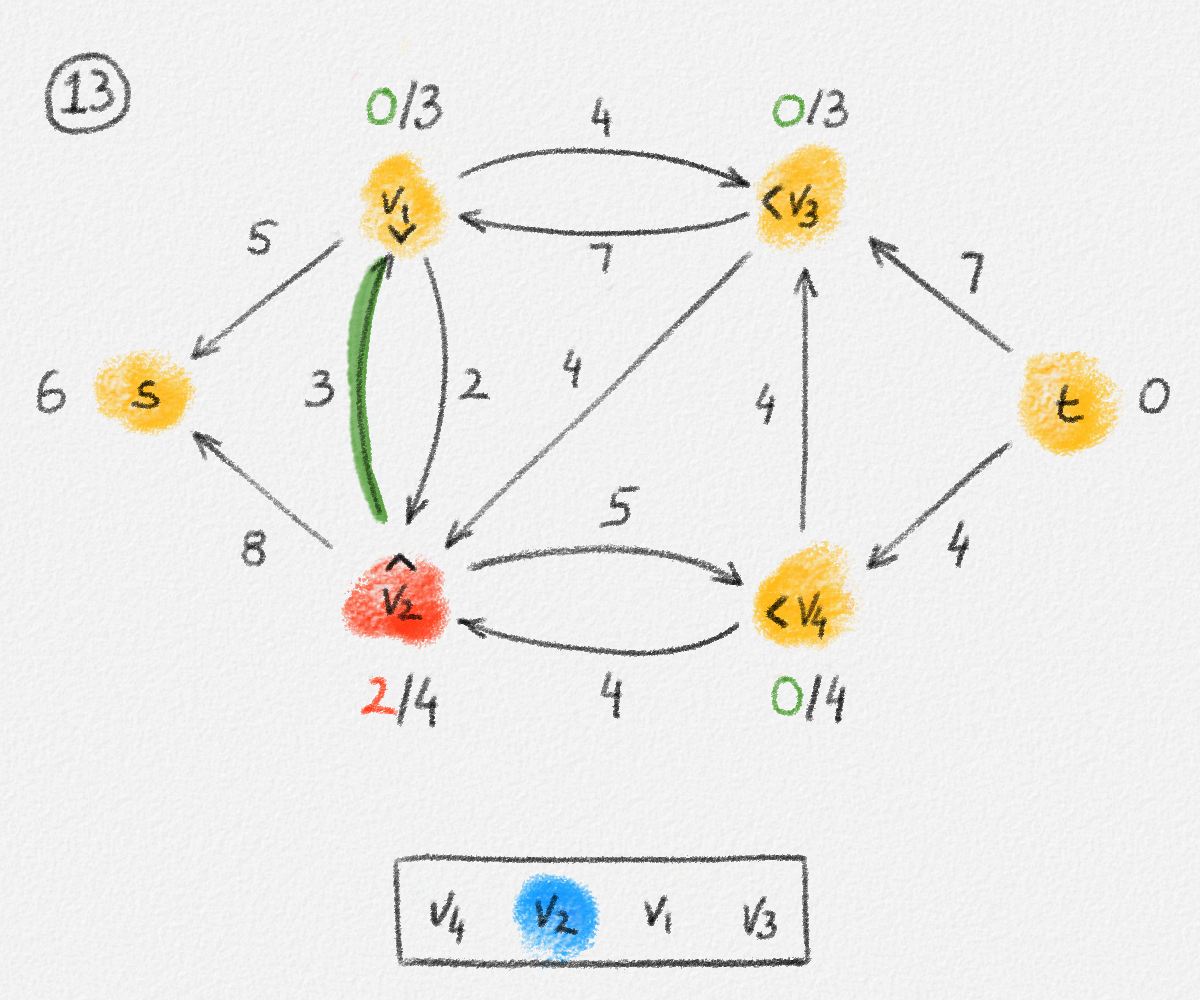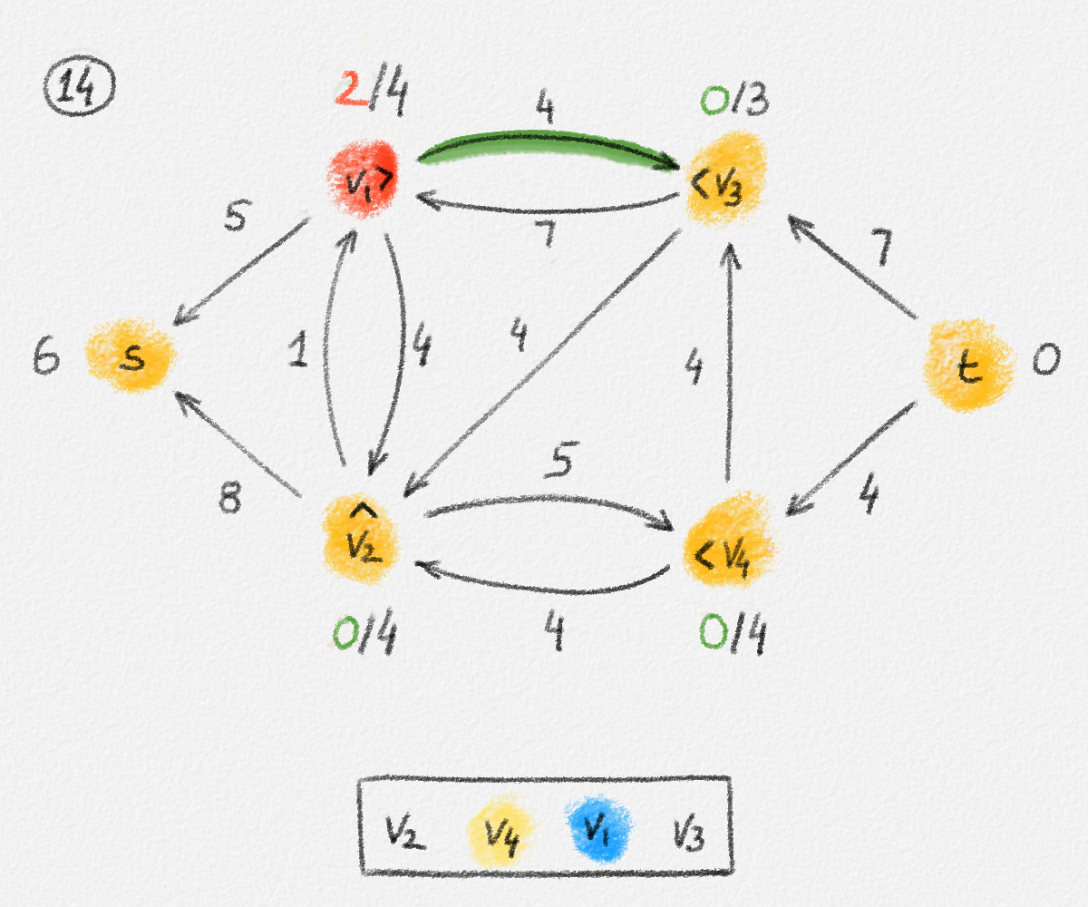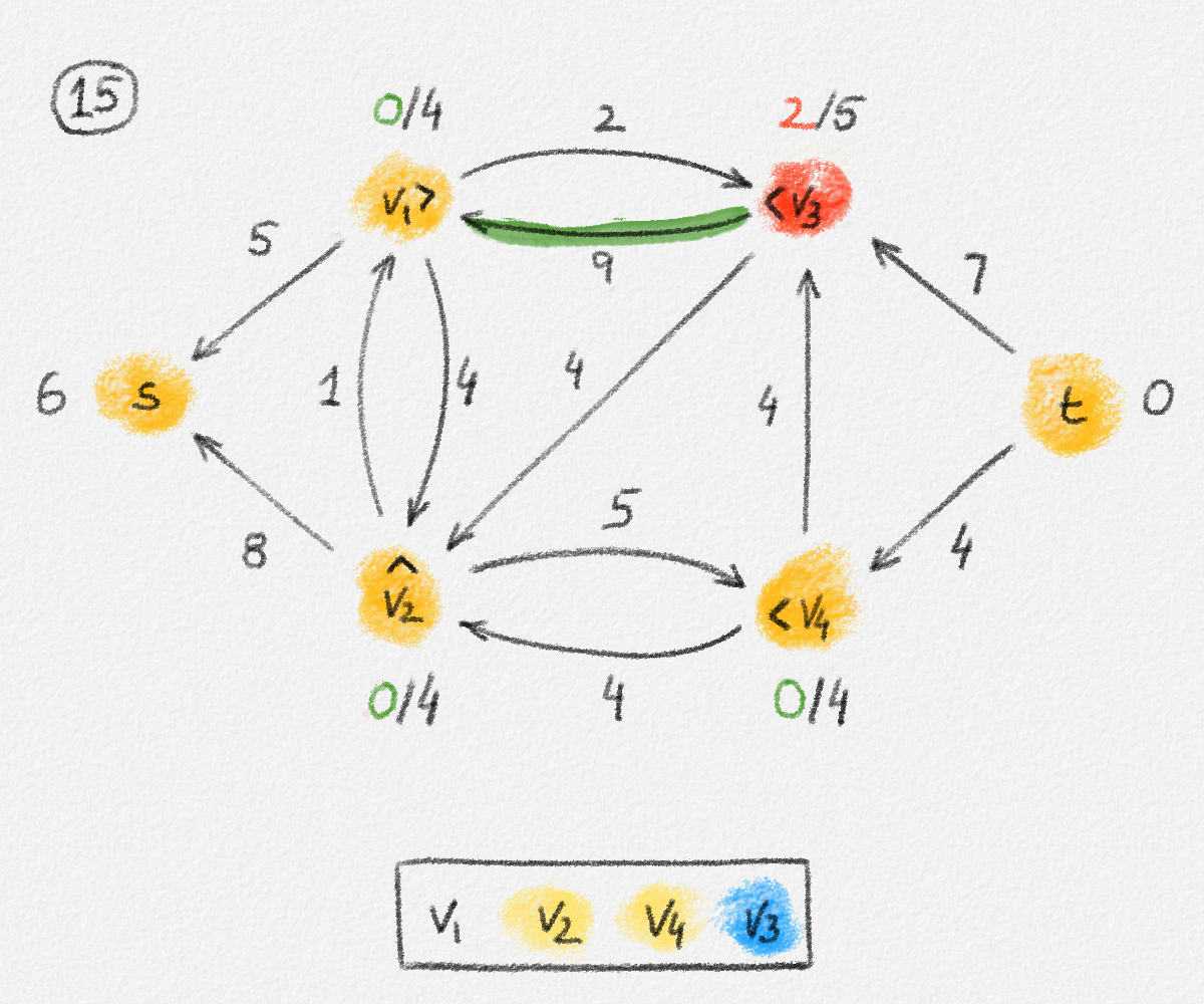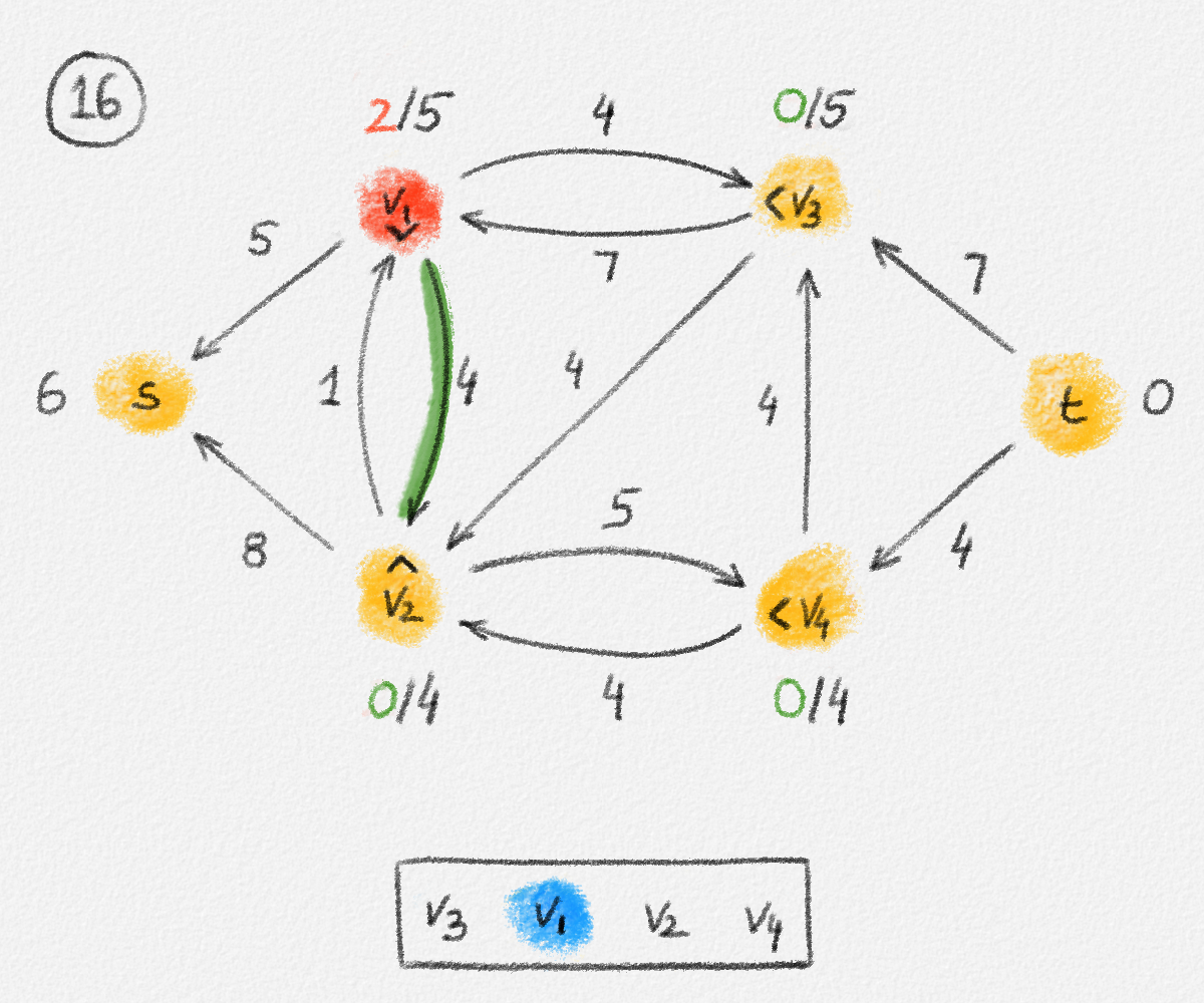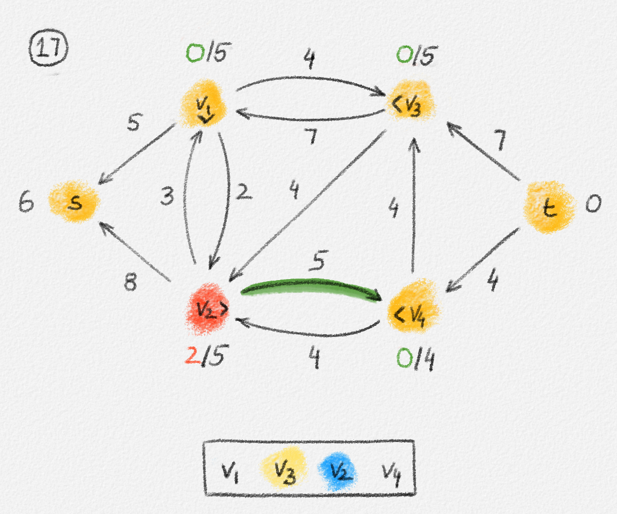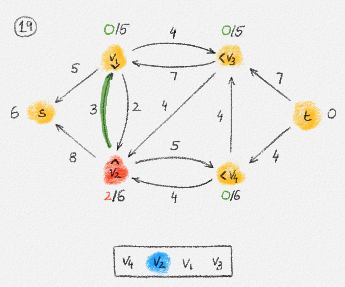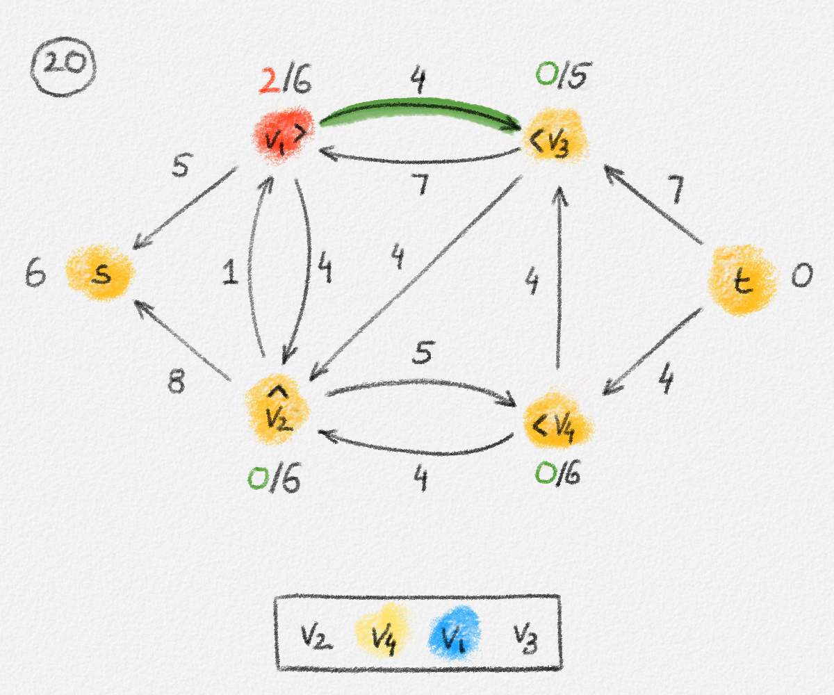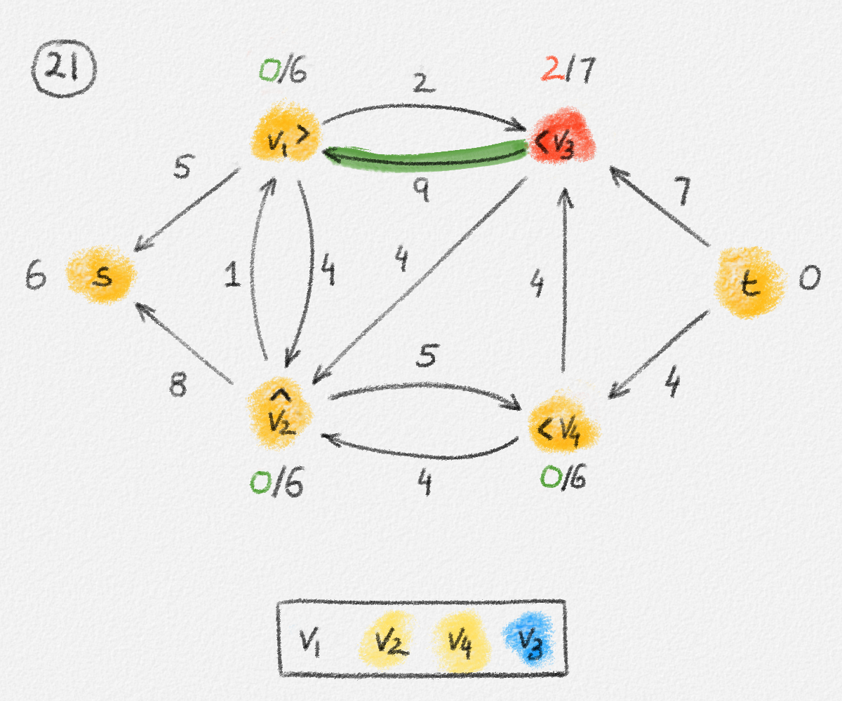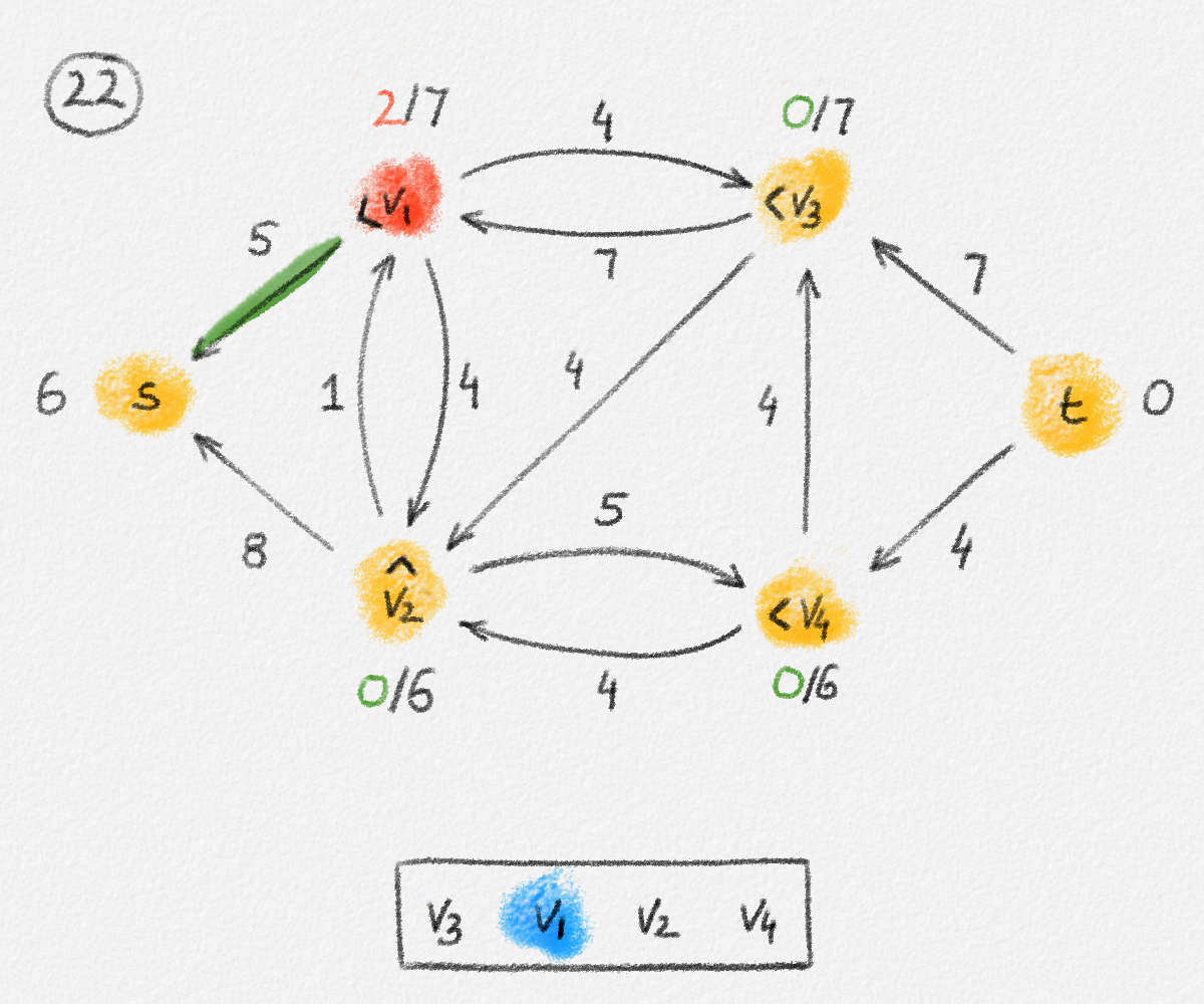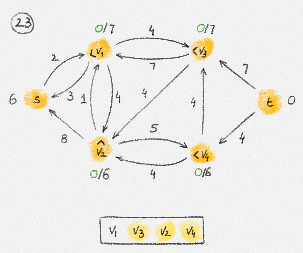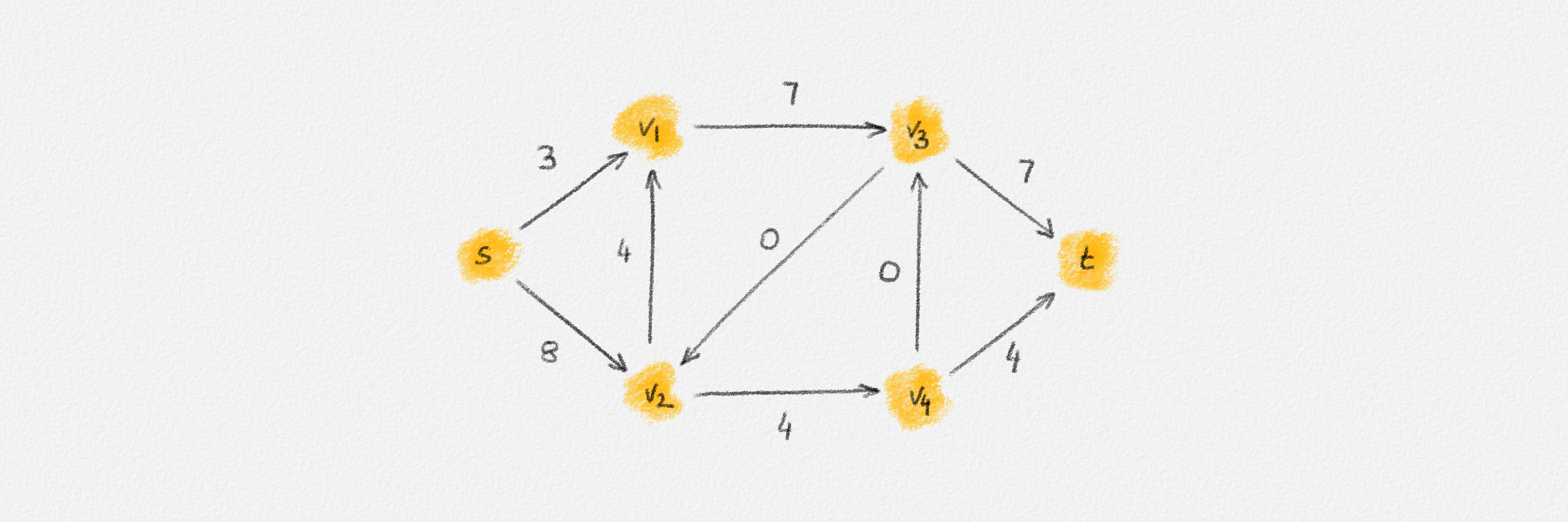Figure 5.17: Illustration of an application of the relabel-to-front algortihm to the network in Figure 5.1. The circled numbers indicate the iteration number. We assume that initially, \(L = \langle v_1, v_2, v_3, v_4\rangle\) and that the vertices in each vertex's neighbour list are sorted by the relation \(s < v_1 < v_2 < v_3 < v_4 < t\). For the different iterations of the algorithm, only the residual network is shown. Edge labels are edge capacities. Black node labels are node heights. Coloured node labels are node excesses, shown in red if positive, and in green if zero. In each figure, the edge used to push flow to a neighbour is shown in red if it is a saturating push, and in green if it is a non-saturating push. If the tail of the edge was relabelled to allow this push to happen, this tail node is shown in red. Every node \(u\) points to its current neighbour \(\textrm{CUR}(u)\) using a small chevron. Finally, for each iteration, the current state of the list \(L\) is shown below the network. The current node is shaded blue. Nodes that were skipped to reach this current node because they have no excess are shaded yellow. The final network on the last row shows the computed flow.

5.2.2.3. Running Time Analysis

Next, let us prove that the algorithm runs in \(O\bigl(n^3\bigr)\) time, as claimed at the beginning of Section 5.2.2. We start by proving that the algorithm performs at most \(O\bigl(n^3\bigr)\) Discharge operations. Since each iteration of the while-loop in the RelabelToFront executes one Discharge operation, this implies that this while-loop runs for at most \(O\bigl(n^3\bigr)\) iterations.

Lemma 5.27: The relabel-to-front algorithm calls Discharge \(O\bigl(n^3\bigr)\) times.

Proof: Let us divide the sequence of calls to the Discharge procedure into phases. The last \(\boldsymbol{\textbf{Discharge}(x)}\) operation in each phase relabels \(x\). All other Discharge operations in a phase do not relabel any vertex. The Discharge operations in the last phase do not relabel any vertex.

Each phase consists of at most \(n\) calls to Discharge. Indeed, no \(\boldsymbol{\textbf{Discharge}(x)}\) operation in this phase, except possibly the last, relabels \(x\). Thus, the vertex \(x\) discharged by this operation is not moved to the front of \(L\) after the \(\boldsymbol{\textbf{Discharge}(x)}\) operation finishes and the distance of the current vertex \(x\) from the head of the list \(L\) increases after each call to \(\boldsymbol{\textbf{Discharge}(x)}\). This can happen at most \(n - 1\) times before \(x = \textrm{NULL}\).

Since the relabel-to-front algorithm is a variant of the generic preflow-push algorithm, Lemma 5.20 shows that the algorithm performs at most \(2n(n-1)\) Relabel operations. Since the last Discharge operation in each phase except the last relabels its argument, this implies that the sequence of calls to Discharge has at most \(2n(n-1) + 1 < 2n^2\) phases. Since each such phase consists of at most \(n\) calls to Discharge, this shows that there are less than \(2n^3\) calls to Discharge. ▨

Using this lemma, we can immediately bound the running time of the relabel-to-front algorithm.

Lemma 5.28: The running time of the relabel-to-front algorithm is \(O\bigl(n^3\bigr)\).

Proof: Excluding the work performed by Discharge operations, the RelabelToFront procedure takes \(O\bigl(n^3\bigr)\) time. Indeed, lines 1–3 take \(O(n)\) time, lines 4–9 take \(O(m) = O\bigl(n^2\bigr)\) time, and each iteration of the while-loop in lines 10–15 takes constant time (excluding the cost of Discharge). Since each iteration of the while-loop performs one Discharge operation, Lemma 5.27 shows that the while-loop runs for \(O\bigl(n^3\bigr)\) iteration, so the cost of lines 10–15 excluding Discharge operations is \(O\bigl(n^3\bigr)\).

A Discharge operation spends all its time in the while-loop in lines 1–8. Each iteration performs one of three actions, so it suffices to bound the total cost of each action summed over all iterations of the while-loop for all vertices.

The first possibility is that the current vertex \(x\) is relabelled in line 3, followed by resetting \(\textrm{CUR}(x)\) to the head of \(\textrm{NBR}(x)\) in line 4. By Exercise 5.2, this takes \(O(n)\) time. By Lemma 5.20, the total number of Relabel operations any preflow-push algorithm performs is \(O\bigl(n^2\bigr)\). Thus, the total cost of lines 3–4 summed over all invocations of Discharge is \(O\bigl(n^3\bigr)\).

The second possible action is to push flow along the current edge \((x, \textrm{CUR}(x))\). By Exercise 5.2, this takes constant time. By Lemma 5.21, there are only \(O(nm) = O\bigl(n^3\bigr)\) saturating Push operations in total. By Observation 5.12, we have \(e_x = 0\) after a non-saturating Push operation, so the Discharge operation returns and we can have at most one non-saturating Push operation per invocation of Discharge. Since Discharge is called \(O\bigl(n^3\bigr)\) times, by Lemma 5.27, this shows that the algorithm performs \(O\bigl(n^3\bigr)\) non-saturating Push operations. The total number of Push operations summed over all invocations of Discharge is thus \(O\bigl(n^3\bigr)\), and the total cost of line 6 summed over all invocations of Discharge is \(O\bigl(n^3\bigr)\).

Finally, consider the cost of line 8. Note that each invocation of line 8 moves \(\textrm{CUR}(x)\) one step closer to the end of \(\textrm{NBR}(x)\). Since \(\textrm{NBR}(x)\) has length at most \(n\), this can happen at most \(n\) times between two consecutive \(\boldsymbol{\textbf{Relabel}(x)}\) operations. Since Lemma 5.20 shows that there are only \(O\bigl(n^2\bigr)\) Relabel operations in total, the cost of line 8 for all invocations of Discharge is thus \(O\bigl(n^3\bigr)\). ▨

5.2.2.4. Correctness of the Algorithm

The last thing to prove is that the relabel-to-front algorithm correctly computes a maximum \(st\)-flow. To this end, we show that the algorithm maintains the following invariant. Let the admissible subgraph \(G^{f,h} = \bigl(V, E^{f,h}\bigr)\) of the residual network \(G^f\) be the subgraph of \(G^f\) whose edge set \(E^{f,h}\) consists of all admissible edges in \(G^f\).

Invariant 5.29: The list \(L\) is a topological ordering of \(G^{f,h}\) and there is no overflowing vertex that precedes the current vertex \(x\) in \(L\).

At the end of the algorithm, \(x\) points one position beyond the end of \(L\), so the invariant states that, at this time, no vertex in \(L\) is overflowing. As shown in the proof of Theorem 5.17, this implies that the edge labelling \(f\) returned by the algorithm is a maximum \(st\)-flow. It remains to prove the invariant.

Proof: Initially, \(h_s = n\) and \(h_x = 0\) for all \(x \ne s\). Since \(n \ge 2\) (\(G\) contains at least \(s\) and \(t\)), there is no edge whose endpoints have heights that differ by exactly one, that is, \(E^{f,h} = \emptyset\). Thus, the arbitrary ordering of the vertices in \(L\) chosen initially is a topological ordering of \(G^{f,h}\). Since \(x\) is the first vertex in \(L\), there is no vertex that precedes \(x\) in \(L\). In particular, no overflowing vertex precedes \(x\) in \(L\).

Next consider the effect of discharging a vertex \(x\) and advancing \(x\) to the next vertex in \(L\). For the sake of clarity, we refer to the value of \(x\) at the beginning of the current iteration as \(x_{\textrm{old}}\) and to the value of \(x\) after the current iteration as \(x_{\textrm{new}}\). We distinguish two cases:

• If \(\boldsymbol{\textbf{Discharge}(x_{\textbf{old}})}\) relabels \(x_{\textrm{old}}\), then \(x_{\textrm{old}}\) is moved to the front of \(L\), so there is no overflowing vertex that precedes \(x_{\textrm{old}}\) in \(L\). Since \(\boldsymbol{\textbf{Discharge}(x_{\textbf{old}})}\) leaves \(x_{\textrm{old}}\) without excess flow, advancing \(x\) from \(x_{\textrm{old}}\) to \(x_{\textrm{new}}\) after the \(\boldsymbol{\textbf{Discharge}(x_{\textbf{old}})}\) operation returns maintains the invariant that there is no overflowing vertex that precedes \(x\) in \(L\).

  By Lemma 5.25, Push operations performed by \(\boldsymbol{\textbf{Discharge}(x_{\textbf{old}})}\) do not create any admissible edges. By Lemma 5.26, the only admissible edges created by relabelling \(x_{\textrm{old}}\) are out-edges of \(x_{\textrm{old}}\). Thus, since \(L\) was a topological ordering of \(G^{f,h}\) before calling \(\boldsymbol{\textbf{Discharge}(x_{\textbf{old}})}\), it remains a topological ordering of \(G^{f,h}\) immediately after \(\boldsymbol{\textbf{Discharge}(x_{\textbf{old}})}\) returns but before moving \(x_{\textrm{old}}\) to the front of \(L\), except that the ordering may violate some out-edges of \(x_{\textrm{old}}\).

  By moving \(x_{\textrm{old}}\) to the front of \(L\), we ensure that the out-edges of \(x_{\textrm{old}}\) are respected by \(L\). By Lemma 5.26, \(x_{\textrm{old}}\) has no admissible in-edges immediately after relabelling \(x_{\textrm{old}}\). By Lemma 5.25, the Push operations performed by \(\boldsymbol{\textbf{Discharge}(x_{\textbf{old}})}\) between the last \(\boldsymbol{\textbf{Relabel}(x_{\textbf{old}})}\) operation and the return of \(\boldsymbol{\textbf{Discharge}(x_{\textbf{old}})}\) cannot make any in-edges of \(x_{\textrm{old}}\) admissible. Thus, \(x_{\textrm{old}}\) has no admissible in-edges after \(\boldsymbol{\textbf{Discharge}(x_{\textbf{old}})}\) returns and \(L\) is a topological ordering of \(G^{f,h}\) after moving \(x_{\textrm{old}}\) to the front of \(L\).

• If \(\boldsymbol{\textbf{Discharge}(x_{\textbf{old}})}\) does not relabel \(x_{\textrm{old}}\), then the ordering of \(L\) is not changed and \(\boldsymbol{\textbf{Discharge}(x_{\textbf{old}})}\) performs only Push operations. By Lemma 5.25, Push operations do not create any admissible edges. Thus, \(L\) remains a topological ordering of \(G^{f,h}\).

  After advancing \(x\) to \(x_{\textrm{new}}\), the vertices preceding \(x\) in \(L\) are \(x_{\textrm{old}}\) and the vertices that precede \(x_{\textrm{old}}\) in \(L\). Since \(\boldsymbol{\textbf{Discharge}(x_{\textbf{old}})}\) leaves \(x_{\textrm{old}}\) without excess flow, this implies that any overflowing vertex \(y\) that precedes \(x_{\textrm{new}}\) must be a vertex that precedes \(x_{\textrm{old}}\) in \(L\). Since there was no overflowing vertex that preceded \(x_{\textrm{old}}\) before the call to \(\boldsymbol{\textbf{Discharge}(x_{\textbf{old}})}\), this Discharge operation must push some flow from \(x_{\textrm{old}}\) to \(y\). Since \(\boldsymbol{\textbf{Discharge}(x_{\textbf{old}})}\) pushes flow only along admissible edges, the edge \((x_{\textrm{old}}, y)\) is thus admissible, a contradiction because \(y\) precedes \(x_{\textrm{old}}\) in \(L\) and \(L\) is a topological ordering of \(G^{f,h}\). This shows that no vertex preceding \(x_{\textrm{new}}\) in \(L\) is overflowing. ▨

As argued above, the relabel-to-front algorithm correctly computes a maximum \(st\)-flow. By Lemma 5.28, its running time is \(O\bigl(n^3\bigr)\). Thus, we obtain the following result:

Theorem 5.30: The relabel-to-front algorithm computes a maximum flow in \(O\bigl(n^3\bigr)\) time.

5.2.3. The Highest-Vertex Preflow-Push Algorithm*

The highest-vertex preflow-push algorithm is the final version of the preflow-push algorithm we discuss. It achieves a running time of \(O\bigl(n^2 \sqrt{m}\bigr)\), which improves on the relabel-to-front algorithm by a factor of up to \(O\bigl(\sqrt{n}\bigr)\). Just as the relabel-to-front algorithm, the algorithm uses Discharge operations to push flow from vertices to their neighbours.¹ While the relabel-to-front algorithm picks vertices to discharge based on the order of vertices in \(L\), the highest-vertex preflow-push algorithm always picks an overflowing vertex with maximum height to be discharged next. Hence its name.

To support picking vertices to discharge based on their heights, we organize \(L\) as an array of linked lists. The \(i\)th linked list stores all overflowing vertices of height \(i\). We also store a height bound \(h_{\textrm{max}}\) and maintain the invariant that all overflowing vertices have height at most \(h_{\textrm{max}}\). Initially, we set \(h_{\textrm{max}} = 0\), which satisfies the invariant because \(s\) does not overflow and any other vertex has height \(0\). To find the next vertex to discharge, we apply the following strategy: As long as \(h_{\textrm{max}} \ge 0\) and there is no overflowing vertex of height \(h_{\textrm{max}}\), we decrease \(h_{\textrm{max}}\) by one. Note that this maintains the property that there is no overflowing vertex of height greater than \(h_{\textrm{max}}\). Thus, if this decreases \(h_{\textrm{max}}\) below zero, then there exists no overflowing vertex and the algorithm exits.

If we stop at a value \(h_{\textrm{max}} \ge 0\), then there exists an overflowing vertex of height \(h_{\textrm{max}}\). We pick such a vertex \(x\), call \(\boldsymbol{\textbf{Discharge}(x)}\), and then repeat the above search for the next vertex to discharge until we finally reach the condition \(h_{\textrm{max}} < 0\).

When calling \(\boldsymbol{\textbf{Discharge}(x)}\) for some vertex \(x\), then \(x\) has height \(h_{\textrm{max}}\) and no overflowing vertex has height greater than \(h_{\textrm{max}}\). Every time \(\boldsymbol{\textbf{Discharge}(x)}\) relabels \(x\), we set \(h_{\textrm{max}} = h_x\) because \(x\) is still overflowing at the time it is relabelled and it is thus the highest overflowing vertex. Every time we push flow from \(x\) to a neighbour \(y\), this makes \(y\)'s excess positive. Thus, we insert \(y\) into the \(h_y\)th list in \(L\) if \(y\)'s excess was not already positive before the Push operation. Note that this does not require an update of \(h_{\textrm{max}}\) because \(x\) has height \(h_{\textrm{max}}\) at any time during the \(\boldsymbol{\textbf{Discharge}(x)}\) operation and, since we push flow from \(x\) to \(y\) only if \(h_y = h_x - 1 < h_{\textrm{max}}\), \(y\) has height less than \(h_{\textrm{max}}\).

On the input graph in Figure 5.1, the highest-vertex preflow-push algorithm performs the same sequence of Push operations as the relabel-to-front algorithm, illustrated in Figure 5.17. The correctness of the algorithm follows immediately because the algorithm returns only once \(h_{\textrm{max}} < 0\), that is, once there is no overflowing vertex left. At this point, \(f\) is a feasible \(st\)-flow. Since the highest-vertex preflow-push algorithm is a variant of the generic preflow-push algorithm, Theorem 5.17 shows that \(f\) is a maximum \(st\)-flow at this point.

5.2.3.1. Running Time Analysis

We divide the analysis of the running time of the highest-vertex preflow-push algorithm into three parts:

• The first part shows that the cost of Relabel and saturating Push operations is \(O(nm)\). (This bound in fact holds for every variant of the generic preflow-push algorithm, but a bound of \(O\bigl(n^3\bigr)\) was sufficient before.)

• The second part of the analysis shows that the highest-vertex preflow-push algorithm performs only \(O\bigl(n^2\sqrt{m}\bigr)\) non-saturating Push operations. As for the generic preflow-push algorithm and for the relabel-to-front algorithm, bounding the number of non-saturating Push operations is the hardest part of the analysis. Since the cost of each such operation is constant, by Exercise 5.2, the cost of these operations is thus \(O\bigl(n^2\sqrt{m}\bigr)\).

• The third part of the analysis shows that the cost of searching \(L\) for the next vertex to be discharged is also \(O\bigl(n^2\sqrt{m}\bigr)\).

Since \(nm \in O\bigl(n^2\sqrt{m}\bigr)\), the cost of the highest-vertex preflow-push algorithm is thus \(O\bigl(n^2\sqrt{m}\bigr)\), as claimed.

Lemma 5.31: The cost of Relabel and saturating Push operations performed by any variant of the generic preflow-push algorithm is \(O(nm)\).

Proof: By Lemma 5.21, the algorithm performs \(O(nm)\) saturating Push operations. Since each such operation takes constant time, by Exercise 5.2, their total cost is \(O(nm)\).

You proved in Exercise 5.2 that the cost of a \(\boldsymbol{\textbf{Relabel}(x)}\) operation is \(O(n)\). If you performed this analysis carefully, you observed that the cost is in fact \(O(\deg(x))\), which is \(O(n)\) because \(\deg(x) < n\). Since every vertex is relabelled at most \(2n\) times, as shown in the proof of Lemma 5.20, the total cost of Relabel operations is thus \(\sum_{x \in V} O(n\deg(x)) = O(nm)\). ▨

Lemma 5.32: The highest-vertex preflow-push algorithm performs \(O\bigl(n^2\sqrt{m}\bigr)\) non-saturating Push operations.

Proof: The analysis uses a potential function \(\Phi\). For every node \(x \in V\), let

\[\ell_x = \bigl|\bigl\{y \in V \mid h_y \le h_x\bigr\}\bigr|\]

be the number of vertices whose heights are no greater than \(x\)'s. Let

\[A = \{ x \in V \setminus \{s, t\} \mid e_x > 0 \}\]

be the set of active vertices, that is, the set of vertices other than \(s\) or \(t\) with positive excess. Then

\[\Phi = \frac{1}{k} \sum_{x \in A} \ell_x,\]

for some parameter \(k\) to be defined later.

Note that \(\Phi \le \frac{n^2}{k}\) initially. Next we consider the effect of Relabel and Push operations on \(\Phi\).

A Push operation does not change the height of any vertex, so \(\ell_x\) remains unchanged for all \(x \in V\). If the Push operation along an edge \((x, y)\) is saturating, then \(x\) remains active and \(y\) may become active if it was not active before. These are the only changes to \(A\). Thus, \(\Phi\) increases by at most \(\frac{\ell_y}{k} \le \frac{n}{k}\). If the Push operation is non-saturating, then again \(\Phi\) increases by at most \(\frac{\ell_y}{k}\) and decreases by \(\frac{\ell_x}{k}\) because \(e_x = 0\) after a saturating \(\boldsymbol{\textbf{Push}(x, y)}\) operation. Since \(h_y = h_x - 1\), we have \(\ell_y < \ell_x\), so \(\Phi\) decreases.

A \(\boldsymbol{\textbf{Relabel}(x)}\) operation increases \(h_x\). This does not change \(A\) and does not increase \(\ell_y\) for any vertex \(y \ne x\). \(\ell_x\) increases by at most \(n\), so \(\Phi\) increases by at most \(\frac{n}{k}\).

Now consider the sequence of Push and Relabel operations the algorithm performs. A phase is a maximal contiguous subsequence of operations during which \(h_{\textrm{max}}\) remains unchanged. We call a phase cheap if it performs at most \(k\) non-saturating Push operations. Otherwise, it is expensive.

Note that \(h_{\textrm{max}} = 0\) initially and increases only as a result of relabelling a vertex \(x\) with \(h_x = h_{\textrm{max}}\). By Lemma 5.20, \(h_{\textrm{max}}\) increases at most \(2n^2\) times. Moreover, the proof of Lemma 5.20 shows that the total increase of \(h_{\textrm{max}}\) over all Relabel operations is at most \(2n^2\). Thus, since \(h_{\textrm{max}}\) remains non-negative while the algorithm runs, \(h_{\textrm{max}}\) also decreases at most \(2n^2\) times. In total, \(h_{\textrm{max}}\) changes at most \(4n^2\) times, so there are at most \(4n^2\) phases. The total number of non-saturating Push operations in cheap phases is therefore at most \(4n^2k\).

For an expensive phase, observe that all Push operations originate at vertices \(x\) with \(h_x = h_{\textrm{max}}\) and no vertices are relabelled during the phase. A non-saturating Push operation originating at a vertex \(x\) deactivates \(x\). In order to perform another non-saturating Push operation from \(x\) to one of its neighbours, \(x\) has to be reactivated, which happens only if \(x\) receives flow from one of its neighbours. However, \(h_x = h_{\textrm{max}}\), we push flow only from vertices with height \(h_{\textrm{max}}\) during this phase, and we push flow only along edges \((y, z)\) with \(h_y = h_z + 1\). Thus, \(x\) does not receive any flow during the current phase and can be the source of at most one non-saturating Push operation in the current phase.

Since we perform more than \(k\) non-saturating Push operations in the current phase and no vertices are relabelled during this phase, this shows that there must exist \(q > k\) vertices of height \(h_{\textrm{max}}\) throughout this phase. Now, as observed above, a non-saturating Push operation along an edge \((x, y)\) decreases \(\Phi\) by \(\frac{\ell_x}{k}\) and increases it by at most \(\frac{\ell_y}{k}\). Since \(h_y = h_x - 1 = h_{\textrm{max}} - 1\), we have

\[\ell_x - \ell_y = |\{z \in V \mid h_z = h_{\textrm{max}}\}| = q.\]

Thus, every non-saturating Push operation in an expensive phase decreases \(\Phi\) by at least \(\frac{q}{k} > 1\).

By Lemmas 5.20 and 5.21, there are \(O(nm)\) Relabel and saturating Push operations and, as argued above, each such operation increases \(\Phi\) by at most \(\frac{n}{k}\) while non-saturating Push operations do not increase \(\Phi\). Thus, \(\Phi\) increases by \(O\Bigl(\frac{n^2m}{k}\Bigr)\) over the course of the algorithm. As observed above, \(\Phi \le \frac{n^2}{k} = O\Bigl(\frac{n^2m}{k}\Bigr)\) initially. Since every non-saturating Push operation in an expensive phase decreases \(\Phi\) by at least \(1\) and \(\Phi \ge 0\) at all times, this implies that the total number of non-saturating Push operations during expensive phases is \(O\Bigl(\frac{n^2m}{k}\Bigr)\).

By summing the number of non-saturating Push operations in cheap and expensive phases, we obtain a bound of \(O\Bigl(n^2k + \frac{n^2m}{k}\Bigr)\) on the total number of non-saturating Push operations. By choosing \(k = \sqrt{m}\), both terms in this sum become \(n^2\sqrt{m}\), that is, the algorithm performs \(O\bigl(n^2\sqrt{m}\bigr)\) non-saturating Push operations. ▨

Lemma 5.33: The cost of searching \(L\) for vertices to be discharged is \(O\bigl(n^2\sqrt{m}\bigr)\).

Proof: Let an iteration consist of decreasing \(h_{\textrm{max}}\) to find the maximum \(h_{\textrm{max}}\) such that \(h_{\textrm{max}} < 0\) or \(L[h_{\textrm{max}}]\) is non-empty, followed by the algorithm exiting or invoking \(\boldsymbol{\textbf{Discharge}(x)}\) for some vertex \(x \in L[h_{\textrm{max}}]\). Let \(h_i'\) be the value of \(h_{\textrm{max}}\) at the beginning of the \(i\)th iteration, and let \(h_i''\) be the value of \(h_{\textrm{max}}\) before the algorithm exits or invokes the \(\boldsymbol{\textbf{Discharge}(x)}\) operation in the \(i\)th iteration. Then the cost of searching \(L\) in the \(i\)th iteration is \(O(1 + \Delta_i)\), where \(\Delta_i = h_i' - h_i''\).

Since every iteration except the last performs a Discharge operation, the number of iterations is one more than the number of Discharge operations the algorithm performs. Since we invoke \(\boldsymbol{\textbf{Discharge}(x)}\) only on vertices \(x\) that overflow, every Discharge operation performs at least one Push operation. By Lemmas 5.21 and 5.32, we perform \(O\bigl(n^2\sqrt{m}\bigr)\) Push operations. Thus, we perform \(O\bigl(n^2\sqrt{m}\bigr)\) Discharge operations and the algorithm runs for \(r = O\bigl(n^2\sqrt{m}\bigr)\) iterations. The total cost of searching \(L\) across all \(r\) iterations is thus

\[\sum_{i=1}^r O(1 + \Delta_i) = O\bigl(n^2\sqrt{m}\bigr) + \sum_{i=1}^r O(\Delta_i).\]

Next we prove that

\[\sum_{i=1}^r \Delta_i = O\bigl(n^2\bigr).\]

Thus, the cost of searching \(L\) across all iterations is \(O\bigl(n^2\sqrt{m}\bigr)\).

To bound \(\sum_{i=1}^r \Delta_i\), we define a potential function

\[\Phi = h_{\textrm{max}} + 2n^2 - \sum_{x \in V} h_x.\]

Initially, \(\Phi \le 2n^2\) because \(h_{\textrm{max}} = 0\) and every vertex has a non-negative height. When the algorithm terminates, \(\Phi \ge 0\) because no vertex has height greater than \(2n - 1\) and \(h_{\textrm{max}} \ge -1\). Every decrease of \(h_{\textrm{max}}\) increases \(\sum_{i=1}^r \Delta_i\) by one and decreases \(\Phi\) by one. When relabelling a vertex \(x\), we have \(h_x = h_{\textrm{max}}\) before and after the Relabel operation. Thus, relabelling \(x\) does not change \(\Phi\), that is, \(\Phi\) never increases. This shows that

\[\sum_{i=1}^r \Delta_i \le 2n^2 = O\bigl(n^2\bigr).\ \text{▨}\]

We are now ready to state the result proven in this section:

Theorem 5.34: The highest-vertex preflow-push algorithm computes a maximum \(st\)-flow in an edge-weighted graph in \(O\bigl(n^2\sqrt{m}\bigr)\) time.

5.3. Existence of Integral Flows*

A question that is important in subsequent chapters is whether we can guarantee that a maximum flow algorithm computes an \(st\)-flow that sends an integral amount of flow across every edge in \(G\). We observe that each of the maximum flow algorithms discussed in this chapter computes an integral maximum flow if all edge capacities are integers.¹

Observation 5.35: If the edge capacities are integers, then the maximum \(st\)-flow computed by any of the algorithms discussed in this chapter sends an integral amount of flow across every edge of \(G\).

Proof: Each maximum flow algorithm starts by setting \(f_{x,y} = 0\) or possibly \(f_{x,y} = u_{x,y}\) if \(x = s\) and the algorithm is a preflow-push algorithm. Thus, initially, the flow across every edge is integral. For a preflow-push algorithm, this in turn implies that the excess of every node is integral.

Every time an augmenting path algorithm changes the current flow \(f\), it sends an amount of flow along the path that matches the minimum residual capacity of the edges on the path. Since the current edge flows and edge capacities are integral, the residual capacities are also integral, so the flow along every edge changes by an integral amount and thus remains integral.

When a preflow-push algorithm changes the flow along an out-edge \((x, y)\) of some overflowing vertex \(x\), the flow it sends along the edge \((x, y)\) is the minimum of \(x\)'s excess and the residual capacity of the edge \((x, y)\). Since both are integral, the flow along the edge \((x, y)\) and the excesses of \(x\) and \(y\) remain integral. ▨

Corollary 5.36: If the edge capacities are integers, then there always exists a maximum flow that sends an integral amount of flow across every edge of \(G\).

6. Minimum-Cost Flows

This chapter is dedicated to another useful variation of network flows. This time, the goal is not to send the maximum amount of flow from one vertex \(s\) to another vertex \(t\) but to send a pre-specified amount of flow from a set of source vertices to a set of sink vertices, at minimum cost.

As a motivating example, consider a car manufacturer's operation. The manufacturer has a number of plants producing cars at different rates; each plant produces a certain number of cars each month. The cars are sold at car dealers with different demands for cars; each dealer sells a certain number of cars each month. Every car dealer needs to be supplied with exactly the number of cars sold and we need to decide which plants ship cars to which dealers. Since the transportation costs to a given dealer differ depending on the plant that sends the car, we want to choose the plants that supply the cars for each dealer so that the overall transportation cost is minimized and the number of cars sent to different dealers by each plant does not exceed the number of cars produced by the plant in each year. We also must not exceed the monthly transportation capacity along the routes between manufacturers and dealers imposed by the transportation network and contracts with logistics companies.

Formally, we can model the transportation network as a directed graph. Every edge \((x, y)\) has a capacity \(u_{x,y}\) and a cost \(c_{x,y}\). We are allowed to send up to \(u_{x,y}\) cars (units of flow) from \(x\) to \(y\) along this edge. The cost of sending \(f_{x,y}\) cars along the edge \((x, y)\) is \(c_{x,y} f_{x,y}\). The total cost of a flow \(f\) is then

\[cf = \sum_{(x, y) \in E} c_{x,y} f_{x,y}\]

(viewing \(c\) and \(f\) as \(m\)-element vectors with one entry per edge).

Every vertex \(x\) has an associated supply balance \(b_x\). If \(b_x\) is positive, \(x\) is a supply vertex (a manufacturer), producing \(b_x\) cars every month. If \(b_x\) is negative, \(x\) is a demand vertex (a car dealer), with demand for \(-b_x\) cars to be sold each month. If \(b_x = 0\), then \(x\) is neither a manufacturer nor a dealer and can only be used as a stop-over for cars travelling from manufacturers to dealers.

For simplicity, we assume that \(\sum_{x \in V} b_x = 0\), that is, the combined supply of all manufacturers exactly matches the demand of all dealers. Then we can formalize the minimum-cost flow problem as the following LP:

Minimum Cost Flow Problem:

\[\begin{gathered} \text{Minimize } cf\\ \begin{aligned} \text{s.t. } 0 \le f_e &\le u_e && \forall e \in E\\ \sum_{y \in V} \bigl(f_{x,y} - f_{y,x}\bigr) &= b_x && \forall x \in V. \end{aligned} \end{gathered}\tag{6.1}\]

Similarly to the maximum flow problem, we refer to the first set of constraints in (6.1) as capacity constraints, and to the second set of constraints as flow conservation constraints (the out-flow of a vertex matches its in-flow plus the flow \(b_x\) it produces).

In general, we allow edges to have infinite capacity \(u_e = \infty\).

An uncapacitated edge is an edge \(e \in E\) with \(u_e = \infty\).

A path made up of only uncapacitated edges is an uncapacitated path.

If all edges are uncapacitated, then we refer to \(G\) as an uncapacitated network.

Similar to the notion of a preflow in Chapter 5, we define:

A pseudo-flow is an edge labelling \(f : E \rightarrow \mathbb{R}^+\) that satisfies the capacity constraints:

\[0 \le f_e \le u_e \quad \forall e \in E.\]

As in Chapter 5,

A flow is an edge labelling \(f : E \rightarrow \mathbb{R}^+\) that satisfies both the capacity constraints,

\[0 \le f_e \le u_e \quad \forall e \in E.\]

and the flow conservation constraints,

\[\sum_{y \in V} \bigl(f_{x,y} - f_{y,x}\bigr) = b_x \quad \forall x \in V.\]

In other words, a flow is any feasible solution of (6.1).

A minimum-cost flow is a flow \(f : E \rightarrow \mathbb{R}^+\) of minimum cost

\[cf = \sum_{e \in E} c_e f_e.\]

Exercise 6.1: Consider a minimum-cost flow problem where the total supply exceeds the total demand, that is, \(\sum_{x \in V} b_x > 0\). In this case, the flow must satisfy all demands, must respect the capacity constraints of all edges, and must not exceed the supply of any vertex. Show how to adapt any minimum-cost flow algorithm for the case when the supply matches the demand to this more general case. In other words, take any minimum-cost flow algorithm as a black box and show how it can be used to solve this general version of the minimum-cost flow problem by providing it with a modified network as input.

In this chapter, we will explore a number of algorithms for computing minimum-cost flows:

• In Section 6.1, we discuss characterizations of minimum-cost flows, that is, conditions that a flow \(f\) satisfies if and only if it is a minimum-cost flow. These characterizations form the basis for the various algorithms we develop.

• In Section 6.2, we show how to express every flow as the sum of a set of very simple flows: path flows that send flow along a single path from a supply vertex to a demand vertex, and cycle flows that send flow along a single cycle in \(G\). This decomposition will be useful in analyzing some of the more advanced algorithms discussed later in this chapter.

• In Section 6.3, we discuss how we can transform the input network so that it satisfies certain properties and so that a solution of the minimum-cost flow problem on the original network can be readily obtained from a solution of the minimum-cost flow problem on the transformed network. Properties we may want to ensure are that there are no edges of negative cost or that the entire network is uncapacitated. This simplifies the description of some of the algorithms in this chapter.

• Section 6.4 finally introduces our first, and rather natural, algorithm for computing a minimum-cost flow, the negative cycle cancelling algorithm. This algorithm starts by constructing an arbitrary feasible flow, which we will see can be done using any maximum flow algorithm. Then we eliminate negative cycles in the residual network by sending flow along such cycles. As shown in Section 6.1.3, once no negative cycle exists, the flow is a minimum-cost flow.

• Section 6.5 introduces our second basic algorithm for computing minimum-cost flows, the successive shortest paths algorithm. This algorithms starts with the trivial pseudo-flow \(f = 0\) and then moves it towards feasibility by moving flow from supply vertices to demand vertices along shortest paths in the residual network.

There is a certain similarity between augmenting path algorithms for computing maximum \(st\)-flows and negative cycle cancelling algorithms in that both start with a feasible flow and improve the flow (by sending flow along augmenting paths or negative-cost cycles in the residual network). Similarly, preflow-push algorithms start with a preflow and move towards feasibility by eliminating excess flow from all vertices to establish flow conservation. Successive shortest paths algorithms start with a pseudo-flow and move towards feasibility by pushing flow from supply vertices to demand vertices along shortest paths in the residual network, again with the goal of establishing flow conservation. More generally, preflow-push and successive shortest paths algorithms are applications of the primal-dual schema, an important technique for designing optimization algorithms that can also be used to obtain approximation algorithms for NP-hard optimization problems.

The basic negative-cycle cancelling algorithm and the basic successive shortest paths algorithm are very simple but efficient only as long as the edge capacities and edge costs are polynomially bounded integer values. There exist numerous improvements over these algorithms, which we cannot all explore in this course. We discuss four of them:

• The first improvement is a simple capacity scaling algorithm, discussed in Section 6.6. This algorithm is important because it introduces a scaling technique to exponentially decrease the dependency of the algorithm's running time on the maximum edge capacity. This is a speed-up technique that can be applied to a wide range of optimization problems.

While capacity scaling speeds up successive shortest paths, it cannot eliminate its dependency on the edge capacities altogether. The remaining three algorithms in this chapter are true polynomial-time algorithms for computing minimum-cost flows, that is, algorithms whose running times depend polynomially on the size of the network but do not depend on the edge capacities and edge costs at all. An important consequence is that they work for arbitrary real-valued edge costs and capacities, not just for integral costs and capacities.

• The minimum-mean cycle cancelling algorithm, discussed in Section 6.7, is a version of negative cycle cancelling that is surprisingly easy to state but requires some care to analyze. It achieves a running time of \(O\bigl(n^2m^3\lg n\bigr)\). The basic idea is to choose the negative cycle along which to send flow in each iteration of the negative cycle cancelling algorithm as the one that minimizes the average (mean) cost of its edges.

• The repeated capacity scaling and enhanced capacity scaling algorithms, discussed in Sections 6.8 and 6.9, achieve significantly better running times and are based on successive shortest paths combined with particular refinements of capacity scaling.

6.1. Characterizations

6.1.1. Complementary Slackness

Complementary slackness is not used directly as the basis for any of the algorithms discussed in this chapter. However, the two optimality criteria that are used in these algorithms are based on complementary slackness. Thus, we start by characterizing a minimum-cost flow using the dual of (6.1) and the corresponding complementary slackness conditions.

For reference, here is (6.1) again, slightly rewritten to split the capacity constraints into upper bound constraints and non-negativity constraints:

\[\begin{gathered} \text{Minimize } cf\\ \begin{aligned} \text{s.t. } f_e &\le u_e && \forall e \in E\\ \sum_{y \in V} \bigl(f_{x,y} - f_{y,x}\bigr) &= b_x && \forall x \in V\\ f_e &\ge 0 && \forall e \in E. \end{aligned} \end{gathered}\tag{6.2}\]

The dual of (6.2) is

\[\begin{gathered} \text{Maximize } \sum_{x \in V} b_x\pi_x - \sum_{(x, y) \in E_b} u_{x,y}s_{x,y}\\ \begin{aligned} \text{s.t. } \pi_x - \pi_y - s_{x,y} &\le c_{x,y} && \forall (x, y) \in E_b\\ \pi_x - \pi_y &\le c_{x,y} && \forall (x, y) \in E_u\\ s_{x,y} &\ge 0 && \forall (x, y) \in E_b, \end{aligned} \end{gathered}\tag{6.3}\]

where \(E_b\) is the set of all edges with finite (bounded) capacity, \(E_u = E \setminus E_b\) is the set of all edges with infinite (unbounded) capacity, \(\pi_x\) is the dual variable associated with the flow conservation constraint of vertex \(x\), and \(s_{x,y}\) is the dual variable associated with the capacity constraint of the edge \((x, y) \in E_b\).

There are no dual variables \(s_{x,y}\) associated with the edge \((x, y) \in E_u\) because the corresponding primal constraint is \(f_{x,y} \le \infty\) and can be omitted (any real number is no greater than infinity).

From here on, we refer to the function \(\pi : V \rightarrow \mathbb{R}\) as a potential function.

Given a cost function \(c : E \rightarrow \mathbb{R}\) and a potential function \(\pi : V \rightarrow \mathbb{R}\), the reduced cost function \(c^\pi\) with respect to \(c\) and \(\pi\) is defined as

\[c^\pi_{x,y} = c_{x,y} - \pi_x + \pi_v \quad \forall x, y \in V.\]

We call a potential function \(\pi\) feasible if there exists a labelling \(s : E_b \rightarrow \mathbb{R}\) such that \((\pi, s)\) is a feasible solution of (6.3).

We call \(\pi\) an optimal potential function if there exists such a feasible solution \((\pi, s)\) of (6.3) that is an optimal solution.

Lemma 6.1: Let \(f\) be a flow in \(G\) and let \(\pi\) be a potential function. Then \(f\) is a minimum-cost flow and \(\pi\) is an optimal potential function for \(G\) if and only if

• \(f_{x,y} = 0\) for every edge \((x, y)\) that satisfies \(c^\pi_{x,y} > 0\) and
• \(f_{x,y} = u_{x,y}\) for every edge \((x, y)\) that satisfies \(c^\pi_{x,y} < 0\).

Note how this lemma captures our intuition about a minimum-cost flow: An edge with positive (reduced) cost should not be used by an optimal flow because this can only increase the cost. An edge with negative (reduced) cost should be used to its maximum capacity because this decreases the cost of the flow.

Proof: For any feasible potential function \(\pi\), let \(s^\pi\) be a labelling of the edges in \(E_b\) such that \(\bigl(\pi, s^\pi\bigr)\) is a feasible solution of (6.3) and there is no feasible solution \((\pi, s)\) that achieves a greater objective function value. In other words, \(\bigl(\pi, s^\pi\bigr)\) is the best solution of (6.3) that satisfies the condition that \(\pi\) is part of this solution.

Observe that every edge \((x, y) \in E_b\) satisfies

\[s^\pi_{x,y} = -c^\pi_{x,y} \text{ or } u_{x,y} = 0.\tag{6.4}\]

Indeed,

\[\pi_x - \pi_y - s^\pi_{x,y} \le c_{x,y},\]

so

\[-s^\pi_{x,y} \le c^\pi_{x,y},\]

that is,

\[s^\pi_{x,y} \ge -c^\pi_{x,y}.\]

Thus, if \(s^\pi_{x,y} \ne -c^\pi_{x,y}\), then \(s^\pi_{x,y} > -c^\pi_{x,y}\). Setting \(s^\pi_{x,y} = -c^\pi_{x,y}\) decreases \(s^\pi_{x,y}\) in this case while still satisfying the constraint that \(\pi_x - \pi_y - s^\pi_{x,y} \le c_{x,y}\).

If \(u_{x,y} > 0\), then decreasing \(s^\pi_{x,y}\) increases the objective function value of \(\bigl(\pi, s^\pi\bigr)\) in (6.3), contradicting the choice of \(s^\pi\). Thus, we can have \(s^\pi_{x,y} > -c^\pi_{x,y}\) only if \(u_{x,y} = 0\).

Now, if \(f\) is a minimum-cost flow and \(\pi\) is an optimal potential function, then \(\pi\) is a feasible potential function, so an edge labelling \(s^\pi\) as above exists. Moreover, since \(\pi\) is an optimal potential function, \(\bigl(\pi, s^\pi\bigr)\) is an optimal solution of (6.3). Thus, by Theorem 4.5,

• Dual complementary slackness: \(f_{x,y} = u_{x,y}\) or \(s^\pi_{x,y} = 0\) for every edge \((x, y) \in E_b\),

• Primal complementary slackness for capacitated edges: \(\pi_x - \pi_y - s^\pi_{x,y} = c_{x,y}\) or \(f_{x,y} = 0\) for every edge \((x, y) \in E_b\), and

• Primal complementary slackness for uncapacitated edges: \(\pi_x - \pi_y = c_{x,y}\) or \(f_{x,y} = 0\) for every edge \((x, y) \in E_u\).

The flow conservation constraints are equality constraints and thus do not introduce any complementary slackness conditions.

To prove that \(f_{x,y} = 0\) for every edge \((x, y)\) that satisfies \(c_{x,y}^\pi > 0\), consider any such edge \((x, y)\). Then \(c_{x,y} >\pi_x - \pi_y\).

If \((x, y) \in E_u\), then primal complementary slackness for uncapacitated edges shows that \(f_{x,y} = 0\).

If \((x, y) \in E_b\), then \(\pi_x - \pi_y \ge \pi_x - \pi_y - s^\pi_{x,y}\) because \(s^\pi_{x,y} \ge 0\), so \(c_{x,y} > \pi_x - \pi_y - s^\pi_{x,y}\). Thus, primal complementary slackness for capacitated edges shows that \(f_{x,y} = 0\).

This proves that \(f_{x,y} = 0\) for every edge \((x, y)\) that satisfies \(c_{x,y}^\pi > 0\).

To prove that \(f_{x,y} = u_{x,y}\) for every edge \((x, y)\) that satisfies \(c^\pi_{x,y} < 0\), consider any such edge \((x, y)\). Then \(c_{x,y} < \pi_x - \pi_y\).

Since \(c_{x,y} \ge \pi_x - \pi_y\) for all \((x, y) \in E_u\), this implies that \((x, y) \in E_b\).

Since \(c_{x,y} \ge \pi_x - \pi_y - s^\pi_{x,y}\) for every edge \((x, y) \in E_b\), we furthermore have that \(s^\pi_{x,y} > 0\). Thus, dual complementary slackness, \(f_{x,y} = u_{x,y}\).

This proves that \(f_{x,y} = u_{x,y}\) for every edge \((x, y)\) that satisfies \(c^\pi_{x,y} < 0\).

We have shown that a minimum-cost flow \(f\) and an optimal potential function \(\pi\) satisfy the conditions of the lemma.

Now assume that \(f\) and \(\pi\) satisfy the conditions of the lemma. We need to prove that \(f\) is a minimum-cost flow and that \(\pi\) is an optimal potential function. By Theorem 4.5, this is the case if \(f\) and \(\bigl(\pi, s^\pi\bigr)\) satisfy the complementary slackness conditions above.

First observe that \(\pi\) is a feasible potential function, so an edge labelling \(s^\pi\) as above exists. Indeed, if \(s\) is the edge labelling defined as

\[s_{x,y} = \begin{cases} 0 & \text{if } c^\pi_{x,y} \ge 0\\ -c^\pi_{x,y} & \text{if } c^\pi_{x,y} < 0, \end{cases}\]

then \((\pi, s)\) is a feasible solution of (6.3): Clearly, \(s_{x,y} \ge 0\) for all \((x, y) \in E_b\). If \((x, y) \in E_u\), then \(f_{x,y} < u_{x,y}\) because \(f_{x,y}\) is finite. Thus, by the second condition of the lemma, \(c^\pi_{x,y} \ge 0\), that is, \(\pi_x - \pi_y \le c_{x,y}\). If \((x, y) \in E_b\), then the choice of \(s_{x,y}\) ensures that \(s_{x,y} \ge -c^\pi_{x,y}\). Thus, \(\pi_x - \pi_y - s_{x,y} \le \pi_x - \pi_y + c^\pi_{x,y} = c_{x,y}\).

Now, to prove that the dual complementary slackness condition holds, consider any edge \((x, y) \in E_b\) such that \(s^\pi_{x,y} > 0\). Then, by (6.4), either \(c^\pi_{x,y} = -s^\pi_{x,y} < 0\) or \(u_{x,y} = 0\). In the former case, \(f_{x,y} = u_{x,y}\), by the second condition of the lemma. In the latter case, \(0 \le f_{x,y} \le u_{x,y} = 0\) because \(f\) is a flow. Thus, again, \(f_{x,y} = u_{x,y}\). This proves that the dual complementary slackness condition holds.

To prove that the primal complementary slackness conditions hold, consider any edge \((x, y)\) such that \(f_{x,y} > 0\). By the first condition of the lemma, this implies that \(c^\pi_{x,y} \le 0\), that is, \(c_{x,y} \le \pi_x - \pi_y\).

If \((x, y) \in E_u\), we have \(c_{x,y} \ge \pi_x - \pi_x\) because \(\pi\) is a feasible potential function. Thus, \(c_{x,y} = \pi_x - \pi_y\). This proves the primal complementary slackness condition for uncapacitated edges.

If \((x, y) \in E_b\), then observe that \(f_{x,y} \le u_{x,y}\). Thus, since \(f_{x,y} > 0\), we have \(u_{x,y} > 0\) and, therefore, \(s^\pi_{x,y} = -c^\pi_{x,y}\), again by (6.4). This implies that \(\pi_x - \pi_y - s^\pi_{x,y} = \pi_x - \pi_y + c_{x,y} - \pi_x - \pi_y = c_{x,y}\). This proves the primal complementary slackness condition for capacitated edges. ▨

6.1.2. The Residual Network and Reduced Costs

The second characterization of a minimum-cost flow uses the reduced costs of edges in the residual network \(G^f\) to decide whether \(f\) is a minimum-cost flow. This network is defined as in Chapter 5, with the added twist that edges in \(G^f\) now have residual costs and the definition of the excess of a vertex is based on the supply balance the vertex started out with in \(G\):

Let \(G = (V, E)\) be a network with vertex supply balances \(b: V \rightarrow \mathbb{R}\), edge capacities \(u : E \rightarrow \mathbb{R}^+\), and edge costs \(c : E \rightarrow \mathbb{R}\), and let \(f : E \rightarrow \mathbb{R}^+\) be a pseudo-flow in \(G\). The residual network of \(G\) with respect to \(f\) is the graph \(G^f = \bigl(V, E^f\bigr)\) with edge set

\[E^f = \{(x, y) \mid (x, y) \in G \text{ and } f_{x,y} < u_{x,y}\} \cup \{(x, y) \mid (y, x) \in G \text{ and } f_{y,x} > 0\}.\]

The residual capacity of an edge \((x, y) \in G^f\) is

\[u^f_{x,y} = u_{x,y} - f_{x,y} + f_{y,x}.\]

The residual cost of an edge \((x, y) \in G^f\) is

\[c^f_{x,y} = \begin{cases} c_{x,y} & \text{if } (x, y) \in G\\ -c_{y,x} & \text{if } (y, x) \in G. \end{cases}\]

The excess (residual supply balance) of a vertex \(x \in V\) is

\[e_x = b_x + \sum_{y \in V} (f_{y,x} - f_{x,y}).\]

We say that a vertex \(x\) is an excess vertex if its excess is positive; \(x\) is a deficit vertex if its excess is negative.

Note that the definition of \(G^f\) and of the residual capacities is identical to the one used in Chapter 5. The definition of the excess of a vertex \(x\) is the same as in Chapter 5, except that we add \(b_x\) to the excess. The definition of the residual cost of an edge has no counterpart in Chapter 5 because there are no edge costs in the maximum flow problem.

One technical difficulty with the construction of \(G^f\) above arises when \(G\) contains both edges \((x, y)\) and \((y, x)\) for two vertices \(x\) and \(y\). In this case, if \((x, y) \in G^f\), we require both that \(c^f_{x,y} = c_{x,y}\) and \(c^f_{x,y} = -c_{y,x}\), which is possible only if \(c_{x,y} = -c_{y,x}\), a condition that may not be satisfied by the input network \(G\). In implementations of the minimum-cost flow algorithms discussed in this chapter, it is easy to sidestep this issue by allowing \(G^f\) to have two copies of the edge \((x, y)\), one representing the edge \((x, y) \in G\) and therefore with cost \(c^f_{x,y} = c_{x,y}\), the other representing the reversal of the edge \((y, x) \in G\) and therefore with cost \(c^f_{x,y} = -c_{y,x}\). In the discussion of the algorithms in this chapter, on the other hand, it is awkward to distinguish between these two edges from \(x\) to \(y\) in \(G^f\). Therefore, we assume that the graph \(G\) contains at most one of the edges \((x, y)\) and \((y, x)\), for every pair of vertices \(x, y \in G\).

If the input graph \(G\) does not satisfy this assumption, we can construct a graph \(G'\) satisfying this assumption by considering every pair of vertices \(x, y \in G\) such that \(G\) contains both edges \((x, y)\) and \((y, x)\) and replacing one of these edges, say \((x, y)\), by two edges \((x, z)\) and \((z, y)\), where \(z\) is a new vertex with supply balance \(b_z = 0\). We set \(u_{x,z} = u_{z,y} = u_{x,y}\), \(c_{x,z} = c_{x,y}\), and \(c_{z,y} = 0\).

Exercise 6.2: Prove that there exists a one-to-one correspondence between feasible flows in \(G\) and in \(G'\), and that any two such flows have the same cost.

Thus, we can find a minimum-cost flow in \(G\) by computing a minimum-cost flow in \(G'\) instead, and \(G'\) satisfies our assumption that there are no two vertices \(x, y \in G'\) such that \(G'\) contains both edges \((x, y)\) and \((y, x)\).

We are now ready to state our next characterization of minimum-cost flows.

Lemma 6.2: A flow \(f\) is a minimum-cost flow if and only if there exists a potential function \(\pi\) such that every edge \((x, y)\) in \(G^f\) has reduced cost \(c^\pi_{x,y} \ge 0\), where the reduced cost of an edge \((x, y)\) is defined as

\[c^\pi_{x,y} = c^f_{x,y} - \pi_x + \pi_y.\]

Proof: First let \(f\) be a minimum-cost flow and let \(\pi\) be an optimal potential function.

Every edge \((x, y) \in G^f\) that is also an edge of \(G\) satisfies \(f_{x,y} < u_{x,y}\). Thus, by the second condition in Lemma 6.1, \(c^\pi_{x,y} \ge 0\).

If \((x, y)\) is not an edge of \(G\), then \((y, x)\) is an edge of \(G\) and \(f_{y,x} > 0\). Thus, by the first condition in Lemma 6.1, \(c^\pi_{y,x} \le 0\). Since \(c^\pi_{x,y} = -c^\pi_{y,x}\), this shows that \(c^\pi_{x,y} \ge 0\) also in this case, that is, the "only if" direction of the lemma holds.

To prove the "if" direction, let \(f\) be a flow and let \(\pi\) be a potential function such that every edge in \(G^f\) satisfies \(c^\pi_{x,y} \ge 0\). Let \((x, y)\) be an edge of \(G\). If \(f_{x,y} > 0\), then \((y, x) \in G^f\), so \(c^\pi_{y,x} \ge 0\) and, therefore, \(c^\pi_{x,y} \le 0\). Thus, \(f\) and \(\pi\) satisfy the first condition in Lemma 6.1.

If \(f_{x,y} < u_{x,y}\), then \((x, y) \in G^f\), so \(c^\pi_{x,y} \ge 0\). Thus, \(f\) and \(\pi\) satisfy the second condition in Lemma 6.1. Since \(f\) and \(\pi\) satisfy both conditions in Lemma 6.1, \(f\) is a minimum-cost flow in \(G\). ▨

6.1.3. Negative Cycles

The final characterization of a minimum-cost flow considers the cost of cycles in the residual network \(G^f\), where the cost of a cycle is the sum of the costs of its edges.

Lemma 6.3: A flow \(f\) is a minimum-cost flow if and only if the residual network \(G^f\) has no negative cycle (cycle of negative cost).

Intuitively, at least the "only if" direction is obvious because, if there exists a negative-cost cycle in \(G^f\), then we can reduce \(f\)'s cost by sending some positive amount of flow \(\delta\) along such a cycle. We can choose \(\delta\) small enough that the resulting modified flow \(f'\) continues to satisfy the capacity constraints. \(f'\) also satisfies the flow conservation constraints because \(f\) does and sending flow along any cycle does not change the net outflow of any vertex.

Proof: First assume that \(f\) is a minimum-cost flow. By Lemma 6.2, there exists a potential function \(\pi\) such that \(c^\pi_{x,y} \ge 0\) for every edge \((x, y) \in G^f\). Next observe that every cycle \(C\) in \(G^f\) satisfies

\[\sum_{(x,y) \in C} c^\pi_{x,y} = \sum_{(x,y) \in C} c^f_{x,y} - \sum_{x \in C} \pi_x + \sum_{y \in C} \pi_y = \sum_{(x, y) \in C} c^f_{x,y}.\]

Since every edge in \(G^f\) satisfies \(c^\pi_{x,y} \ge 0\), the first sum is non-negative, that is, \(G^f\) contains no negative cycle.

Now assume that \(G^f\) contains no negative cycle. Then we transform \(G^f\) into a graph \(H^f\) by choosing a distinguished vertex \(s \in V\) and adding an edge from \(s\) to every vertex \(x \in V \setminus \{s\}\). Choose the cost of each such edge \((s, x)\) to be equal to \(\sum_{e \in G^f} \bigl|c^f_e\bigr|\). Then every vertex in \(H^f\) is reachable from \(s\) and \(H^f\) contains no negative cycle. Indeed, any cycle that contains only edges in \(G^f\) has a non-negative cost. Any cycle that includes at least one edge \((s, x)\) has cost at least

\[\sum_{e \in G^f} \Bigl|c^f_e\Bigr| + \sum_{\substack{e \in G^f\\c^f_e < 0}} c^f_e \ge 0.\]

Since every vertex is reachable from \(s\) in \(H^f\) and \(H^f\) has no negative cycles, every vertex \(x \in V\) has a well defined distance \(d_x\) from \(s\) in \(H_f\) with respect to the edge costs as edge lengths. We define a potential function \(\pi\) as

\[\pi_x = -d_x \quad \forall x \in V.\]

Then every edge \((x, y)\) in \(H^f\) satisfies

\[d_y \le d_x + c^f_{x,y},\]

that is,

\[c^\pi_{x,y} = c_{x,y}^f - \pi_x + \pi_y \ge 0.\]

Since every edge of \(G^f\) is also an edge of \(H^f\), this shows that \(f\) and \(\pi\) satisfy the condition of Lemma 6.2, so \(f\) is a minimum-cost flow in \(G\). ▨

6.2. Decomposing Flows*

This section introduces a useful tool we will use in analyzing some of the algorithms in this chapter.

So far, we have viewed a flow as a collection of individual flow amounts sent along the edges of the graph, as a function \(f: E \rightarrow \mathbb{R}\). This function cannot be completely arbitrary. To be a flow, it needs to satisfy the capacity and flow conservation constraints. If you think back to augmenting path algorithms, we did not construct a maximum flow one edge at a time. Instead, we chose a set of paths from \(s\) to \(t\) and an amount of flow to be sent along each path. The final flow was then the sum of these "path flows".

When computing minimum-cost flows, we no longer have a single source or a single sink. Instead, we have supply vertices and demand vertices and, as we show in this section, we can once again obtain a feasible flow as the sum of a collection of path flows from supply vertices to demand vertices. The total flow along all paths starting at each supply vertex must match its supply. The total flow along all paths ending at a demand vertex must match its demand. Since we want to compute a minimum-cost flow, there is an added twist. Once we have found a feasible flow that routes flow along paths from supply vertices to demand vertices, we may be able to reduce its cost by sending some flow from a vertex back to itself along a negative-cost cycle. This does not alter the supply balance at any vertex, but it reduces the cost of the flow. Thus, in general, every flow can be decomposed into a collection of paths and cycles. The remainder of this section proves this formally.

• In Section 6.2.1, we introduce the concepts of circulations, cycle flows, and path flows.

• In Section 6.2.2, we prove that every pseudo-flow can be represented as the sum of a bounded number of path and cycle flows.

• Section 6.2.3 explores the relationship between pseudo-flows, flows, and circulations in their residual networks.

6.2.1. Circulations

A circulation in a network \(G\) is a pseudo-flow \(f\) that satisfies

\[\sum_{y \in V} \bigl(f_{x,y} - f_{y,x}\bigr) = 0 \quad \forall x \in V.\]

In other words, no vertex produces or absorbs any flow; the flow simply circulates through the network.

A cycle flow is a circulation \(f\) in \(G\) such that the edges \(e \in G\) with \(f_e > 0\) form a simple cycle in \(G\).

A path flow is a pseudo-flow \(f\) in \(G\) such that the edges \(e \in G\) with \(f_e > 0\) form a simple path \(P\) in \(G\) and, for every vertex \(x\) of \(G\) except the endpoints of \(P\),

\[\sum_{y \in V} \bigl(f_{x,y} - f_{y,x}\bigr) = 0.\]

6.2.2. Decomposition into Cycles and Paths

In this section, we prove that every flow can be written as a sum of a bounded number of cycle flows and path flows. To prove this, we need the following lemma, which states that, as long as there exist supply and demand vertices, every flow sends a positive amount of flow along some path from a supply vertex to a demand vertex:

Lemma 6.4: If \(f\) is a flow in a network \(G\) and \(b_x \ne 0\) for some vertex \(x \in G\), then there exists a path \(P\) in \(G\) from a supply vertex to a demand vertex such that \(f_e > 0\) for every edge \(e \in P\).

Proof: Since \(\sum_{x \in V} b_x = 0\), the existence of a supply vertex implies that there must exist a demand vertex and vice versa. Thus, if there exists a vertex \(x\) with \(b_x \ne 0\), we can choose \(x\) to be a supply vertex. Let \(R\) be the set of vertices reachable from \(x\) in the subgraph \(G^+ = (V, E^+)\), where \(E^+ = \{ e \in E \mid f_e > 0 \}\) is the set of edges in \(G\) used by \(f\). If \(R\) contains a demand vertex \(y\), then there exists a path \(P\) from \(x\) to \(y\) consisting of only edges in \(E^+\) and the lemma holds. If \(R\) contains no demand vertex, then \(R\) is a cut of \(G\) because \(x \in R\) and \(G\) has at least one demand vertex, which must be in \(V \setminus R\). Since \(x \in R\), \(b_x > 0\), and \(b_y \ge 0\) for all \(y \in R\), we have

\begin{align} 0 &< \sum_{y \in R} b_y\\ &= \sum_{y \in R} \sum_{z \in V} \bigl(f_{y,z} - f_{z,y}\bigr)\\ &= \sum_{y \in R} \sum_{z \in R} \bigl(f_{y,z} - f_{z,y}\bigr) + \sum_{y \in R} \sum_{z \notin R} \bigl(f_{y,z} - f_{z,y}\bigr)\tag{6.5}\\ &= \sum_{y \in R} \sum_{z \notin R} \bigl(f_{y,z} - f_{z,y}\bigr)\tag{6.6}\\ &\le \sum_{y \in R} \sum_{z \notin R} f_{y,z}.\tag{6.7} \end{align}

(6.6) follows because the first sum in (6.5) contains the flow along every edge \((y, z)\) with \(y, z \in R\) twice, once with positive sign and once with negative sign. Thus, this sum is zero. (6.7) follows because \(f_{z,y} \ge 0\) for every pair of vertices \(y, z \in V\).

Since \(\sum_{y \in R} \sum_{z \notin R} f_{y,z} > 0\), there exists an edge \((y, z)\) with \(y \in R\) and \(z \notin R\) such that \(f_{y,z} > 0\), a contradiction. ▨

The next lemma states the main claim of this section: that every pseudo-flow \(f\) can be decomposed into a collection of path and cycle flows. It also provides a bound on the number of path and cycle flows in the decomposition and states that there exists such a decomposition consisting of only cycle flows if \(f\) is a circulation.

Lemma 6.5: Any pseudo-flow \(f\) in a network \(G\) can be represented as a sum of \(t \le n + m\) path or cycle flows \(f^{(1)}, \ldots, f^{(t)}\) in \(G\). If \(f\) is a circulation, then \(t \le m\) and \(f^{(1)}, \ldots, f^{(t)}\) are all cycle flows.

Proof: Consider a vertex supply balance function \(b\) defined as

\[b_x = \sum_{y \in V} \bigl(f_{x,y} - f_{y,x}\bigr).\]

Then \(f\) is a flow with respect to this vertex supply balance function. Let \(\Phi(f)\) be the number of edges \(e \in G\) such that \(f_e > 0\) and let \(\Psi(f)\) be the number of supply and demand vertices with respect to \(b\). We have \(\Phi(f) \le m\) and \(\Psi(f) \le n\). The first part of the proof uses induction on \(\Psi(f) + \Phi(f)\) to show that any pseudo-flow \(f\) can be written as the sum of a circulation \(f'\) plus \(t_1 \le \Psi(f) + \Phi(f) - \Phi(f')\) path flows \(p^{(1)}, \ldots, p^{(t_1)}\). The second part of the proof uses induction on \(\Phi(f')\) to show that any circulation \(f'\) can be written as the sum of \(t_2 \le \Phi(f')\) cycle flows \(o^{(1)}, \ldots, o^{(t_2)}\). Together, these two claims show that \(f\) can be written as the sum of \(t_1 + t_2 \le \Psi(f) + \Phi(f) - \Phi(f') + \Phi(f') = \Psi(f) + \Phi(f) \le n + m\) cycle and path flows \(p^{(1)}, \ldots, p^{(t_1)}, o^{(1)}, \ldots, o^{(t_2)}\). Moreover, if \(f\) is a circulation, then \(\Psi(f) = 0\), so we obtain a decomposition of \(f\) into \(t_2 \le \Phi(f) \le m\) cycle flows \(o^{(1)}, \ldots, o^{(t_2)}\).

Decomposing \(\boldsymbol{f}\) into a circulation and path flows: If \(\Psi(f) = 0\), then \(f\) is a circulation and can thus be written as the sum of \(f\) itself and \(0 = \Psi(f) + \Phi(f) - \Phi(f)\) path flows. So assume that \(\Psi(f) > 0\). By Lemma 6.4, there exists a path \(P\) in \(G\) from a supply vertex \(x\) to a demand vertex \(y\) such that \(f_e > 0\) for every edge \(e \in P\). Let

\[\delta = \min (\{ b_x, -b_y \} \cup \{ f_e \mid e \in P \}),\]

let \(p^{(1)}\) be the path flow defined as

\[p^{(1)}_e = \begin{cases} \delta & \text{if } e \in P\\ 0 & \text{otherwise,} \end{cases}\]

and let \(f'' = f - p^{(1)}\).

\(p^{(1)}\) is easily seen to be a path flow: We have \(0 \le p^{(1)}_e \le f_e \le u_e\) for every edge \(e \in G\) because \(f\) is a pseudo-flow, every vertex \(z \notin \{x, y\}\) satisfies

\[\sum_{z \in V} \bigl(f_{z,w} - f_{w,z}\bigr) = 0,\]

and the edges with \(p^{(1)}_e > 0\) form the path \(P\).

\(f''\) is a pseudo-flow because \(0 \le p^{(1)}_e \le f_e\) for every edge \(e \in G\), so \(0 \le f''_e = f_e - p^{(1)}_e \le f_e \le u_e\) for every edge \(e \in G\).

The vertex supply balance function \(b''\) defined as

\[b''_z = \begin{cases} b_z - \delta & \text{if } z = x\\ b_z + \delta & \text{if } z = y\\ b_z & \text{if } z \notin \{x, y\} \end{cases}\]

turns \(f''\) into a flow. Moreover, we have \(\Phi(f'') \le \Phi(f)\) and \(\Psi(f'') \le \Psi(f)\), and at least one of these two inequalities is strict. Indeed, if \(\delta = b_x\) or \(\delta = -b_y\), then \(\Psi(f'') < \Psi(f)\); if \(\delta = f_e\) for some edge \(e \in P\), then \(\Phi(f'') < \Phi(f)\). Thus, \(\Phi(f'') + \Psi(f'') < \Phi(f) + \Psi(f)\) and, by the induction hypothesis, \(f''\) can be written as the sum of a circulation \(f'\) and \(t_1 - 1 \le \Psi(f'') + \Phi(f'') - \Phi(f') \le \Psi(f) + \Phi(f) - \Phi(f') - 1\) path flows \(p^{(2)}, \ldots, p^{(t_1)}\). Since \(f = p^1 + f''\) and \(p^{(1)}\) is a path flow, \(f\) can therefore be written as the sum of \(f'\) and \(t_1 \le \Psi(f) + \Phi(f) - \Phi(f')\) path flows \(p^{(1)}, \ldots, p^{(t_1)}\).

Decomposing a circulation into cycles: Let \(f'\) be a circulation. If \(\Phi(f') = 0\), then \(f'_e = 0\) for every edge \(e \in G\) and \(f'\) can be written as the sum of \(0 = \Phi(f')\) cycle flows. If \(\Phi(f') > 0\), then let \(G^+ = (V, E^+)\), where \(E^+ = \{ e \in E \mid f'_e > 0 \}\) is the set of edges used by \(f'\). Since \(f'\) is a circulation, \(G^+\) has no vertex with only in-edges or only out-edges. Thus, since \(\Phi(f') > 0\) and therefore \(E^+ \ne \emptyset\), there exists a cycle \(C\) in \(G^+\). Let \(\delta = \min_{e \in C} f'_e\). Then we define \(o^{(1)}\) as

\[o^{(1)}_e = \begin{cases} \delta & \text{if } e \in C\\ 0 & \text{otherwise} \end{cases}\]

and \(f''\) as \(f'' = f' - o^{(1)}\).

\(o^{(1)}\) is easily seen to be a cycle flow: All edges satisfy their capacity constraints, every vertex \(x \in V\) satisfies

\[\sum_{y \in V} \bigl(f_{x,y} - f_{y,x}\bigr) = 0,\]

and the edges with \(o^{(1)}_e > 0\) form the cycle \(C\).

Since both \(f'\) and \(o^{(1)}\) are circulations, we have

\[\sum_{y \in V} \bigl(f''_{x,y} - f''_{y,x}\bigr) = \sum_{y \in V} \bigl(f'_{x,y} - f'_{y,x}\bigr) - \sum_{y \in V} \Bigl(o^{(1)}_{x,y} - o^{(1)}_{y,x}\Bigr) = 0 \quad \forall x \in V.\]

By an argument similar to the first part of the proof, \(f''\) also satisfies the capacity constraints of \(G\). Thus, \(f''\) is a circulation in \(G\).

Since \(f'_e = \delta\) for at least one edge \(e \in C\), we have \(\Phi(f'') < \Phi(f')\). Thus, by the induction hypothesis, \(f''\) can be written as the sum of \(t_2 - 1 \le \Phi(f'') \le \Phi(f') - 1\) cycle flows \(o^{(2)}, \ldots, o^{(t_2)}\). Since \(o^{(1)}\) is a cycle flow and \(f' = f'' + o^{(1)}\), \(f'\) can thus be written as the sum of \(t_2 \le \Phi(f')\) cycle flows \(o^{(1)}, \ldots, o^{(t_2)}\). ▨

6.2.3. Flows and Circulations in the Residual Network

The next two lemmas establish essentially that we can arrive at a flow in \(G\) by starting with any pseudo-flow \(f\) (e.g., \(f_e = 0\) for all \(e \in G\)) and then repeatedly augmenting it with a flow in the residual network \(G^f\). They show that the difference between two pseudo-flows in a network is a pseudo-flow in the residual network of one of the two flows.

Lemma 6.6: For two pseudo-flows \(f\) and \(f'\) in \(G\), the edge labelling \(\delta\) defined as

\[\delta_{x,y} = \max\bigl(0, f'_{x,y} - f'_{y,x} - f_{x,y} + f_{y,x}\bigr)\]

is a pseudo-flow in \(G^f\). If \(f'\) is a flow, then so is \(\delta\). If both \(f\) and \(f'\) are flows, then \(\delta\) is a circulation.

Proof: First we prove that \(\delta\) is a pseudo-flow in \(G^f\). By definition, \(\delta_{x,y} \ge 0\) for every edge \((x, y) \in G^f\). Since \(f\) is a pseudo-flow, we have \(f_{x,y} \le u_{x,y}\) and \(f_{y,x} \ge 0\) for every edge \((x, y) \in G^f\). Thus,

\[u^f_{x,y} = u_{x,y} - f_{x,y} + f_{y,x} \ge 0.\]

If \(\delta_{x,y} = 0\), this implies that \(\delta_{x,y} \le u^f_{x,y}\). If \(\delta_{x,y} > 0\), then

\[\begin{aligned} \delta_{x,y} &= f'_{x,y} - f'_{y,x} - f_{x,y} + f_{y,x}\\ &\le f'_{x,y} - f_{x,y} + f_{y,x}\\ &\le u_{x,y} - f_{x,y} + f_{y,x}\\ &= u^f_{x,y} \end{aligned}\]

because \(f'\) is a pseudo-flow and thus \(f'_{y,x} \ge 0\) and \(f'_{x,y} \le u_{x,y}\). This proves that \(\delta\) is a pseudo-flow in \(G^f\).

To prove that \(\delta\) is a flow if \(f'\) is a flow, let \(\delta'_{x,y} = f'_{x,y} - f_{x,y}\). Then \(\delta_{x,y} = \max\bigl(0, \delta'_{x,y} - \delta'_{y,x}\bigr)\) for every edge \((x, y) \in G^f\). Thus, for all \(x \in V\),

\begin{align} \sum_{y \in V} \Bigl(\delta_{x,y} - \delta_{y,x}\Bigr) &= \sum_{y \in V} \biggl(\max\Bigl(0, \delta'_{x,y} - \delta'_{y,x}\Bigr) - \max\Bigl(0, \delta'_{y,x} - \delta'_{x,y}\Bigr)\biggr)\\ &= \sum_{y \in V} \Bigl(\delta'_{x,y} - \delta'_{y,x}\Bigr)\\ &= \sum_{y \in V} \biggl(\Bigl(f'_{x,y} - f_{x,y}\Bigr) - \Bigl(f'_{y,x} - f_{y,x}\Bigr)\biggr)\\ &= \sum_{y \in V} \Bigl(f'_{x,y} - f'_{y,x}\Bigr) - \sum_{y \in V} \Bigl(f_{x,y} - f_{y,x}\Bigr)\\ &= b_x - \sum_{y \in V} \Bigl(f_{x,y} - f_{y,x}\Bigr)\tag{6.8}\\ &= e_x. \end{align}

(6.8) follows because \(f'\) is a flow, that is, it satisfies the flow conservation constraints in \(G\). Thus, \(\delta\) satisfies the flow conservation constraints in \(G^f\) and, being a pseudo-flow in \(G^f\), is a flow in \(G^f\).

Finally, assume that both \(f\) and \(f'\) are flows in \(G\). By the above argument, \(\delta\) is a flow in \(G^f\). Since \(f\) is a flow, \(e_x = 0\) for all \(x \in V\), which implies that

\[\sum_{y \in V} \bigl(\delta_{x,y} - \delta_{y,x}\bigr) = e_x = 0 \quad \forall x \in V,\]

that is, \(\delta\) is a circulation. ▨

Lemma 6.7: If \(f\) is a pseudo-flow in \(G\) and \(\delta\) is a pseudo-flow in \(G^f\), then the edge labelling \(f'\) defined as

\[f'_{x,y} = f_{x,y} + \delta_{x,y} - \delta_{y,x} \quad \forall (x, y) \in G\]

is a pseudo-flow in \(G\) of cost

\[\sum_{e \in G} c_ef_e + \sum_{e \in G^f} c^f_e\delta_e.\]

If \(f\) is a flow and \(\delta\) is a circulation, then \(f'\) is a flow.

Proof: First we prove that \(f'\) is a pseudo-flow in \(G\).

Consider any edge \((x,y) \in G\). Since \((x,y) \in G\), we have \((y,x) \notin G\), that is, \(f_{y,x} = u_{y,x} = 0\). Since \(\delta\) is a pseudo-flow in \(G^f\), we have

\[0 \le \delta_{x,y} \le u^f_{x,y} = u_{x,y} - f_{x,y}\]

and

\[0 \le \delta_{y,x} \le u^f_{y,x} = f_{x,y}.\]

Thus,

\[f'_{x,y} \le f_{x,y} + u_{x,y} - f_{x,y} = u_{x,y}\]

and

\[f'_{x,y} \ge f_{x,y} - f_{x,y} = 0.\]

This proves that \(f'\) is a pseudo-flow.

Next assume that \(f\) is a flow and \(\delta\) is a circulation. Then

\[\begin{aligned} \sum_{(x,y) \in G}f'_{x,y} - \sum_{(y,x) \in G} f'_{y,x} &= \sum_{(x,y) \in G} \bigl(f_{x,y} + \delta_{x,y} - \delta_{y,x}\bigr) - \sum_{(y,x) \in G} \bigr(f_{y,x} + \delta_{y,x} - \delta_{x,y}\bigr)\\ &= \sum_{(x,y) \in G} f_{x,y} - \sum_{(y,x) \in G} f_{y,x} + \sum_{(x,y) \in G} \bigl(\delta_{x,y} - \delta_{y,x}\bigr) + \sum_{(y,x) \in G} \bigl(\delta_{x,y} - \delta_{y,x}\bigr)\\ &= b_x. \end{aligned}\]

Thus, \(f'\) satisfies the flow conservation constraints. Being a pseudo-flow, it is therefore a flow.

Finally, consider the cost of \(f'\). Since \(c^f_{x,y} = c_{x,y}\) and \(c^f_{y,x} = -c_{x,y}\) for every edge \((x,y) \in G\), we have

\[\begin{aligned} \sum_{(x,y) \in G} c_{x,y} f'_{x,y} &= \sum_{(x,y) \in G} c_{x,y}f_{x,y} + \sum_{(x,y) \in G} c_{x,y}\delta_{x,y} - \sum_{(x,y) \in G} c_{x,y}\delta_{y,x}\\ &= \sum_{(x,y) \in G} c_{x,y} f_{x,y} + \sum_{(x,y) \in G} c^f_{x,y}\delta_{x,y} + \sum_{(x,y) \in G} c^f_{y,x}\delta_{y,x}\\ &= \sum_{e \in G} c_ef_e + \sum_{e \in G^f} c^f_e\delta_e.\ \text{▨} \end{aligned}\]

The final lemma in this section will be used in the correctness proof of the enhanced capacity scaling algorithm in Section 6.9. Intuitively, this lemma says that a pseudo-flow \(\delta\) in the residual network \(G^f\) of a pseudo-flow \(f\) can be reversed (sending flow from \(y\) to \(x\) if \(\delta\) sends flow from \(x\) to \(y\)) to obtain a pseudo-flow \(\delta^r\) in the residual network \(G^{f'}\) of another pseudo-flow \(f'\) provided that \(\delta\) is "bounded by the difference between \(f'\) and \(f\)".

Lemma 6.8: Let \(f\) and \(f'\) be pseudo-flows in \(G\) and let \(\delta\) be a pseudo-flow in \(G^f\) such that

\[\delta_{x,y} \le \max\Bigl(0, \bigl(f'_{x,y} - f'_{y,x}\bigr) - \bigl(f_{x,y} - f_{y,x}\bigr)\Bigr) \quad \forall (x, y) \in G^f.\]

Then the function \(\delta^r\) defined as \(\delta^r_{x,y} = \delta_{y,x}\) is a pseudo-flow in \(G^{f'}\). If \(\delta\) is a circulation, cycle flow or path flow, then so is \(\delta^r\).

Proof: As in the proof of Lemma 6.6, let \(\delta'_{x,y} = f'_{x,y} - f_{x,y}\). Then \(0 \le \delta_{x,y} \le \max\bigl(0, \delta'_{x,y} - \delta'_{y,x}\bigr)\). Thus, since \(\delta^r_{y,x} = \delta_{x,y}\), \(\delta^r\) is a pseudo-flow in \(G^{f'}\) if \(\max\bigl(0, \delta'_{x,y} - \delta'_{y,x}\bigr) \le u^{f'}_{y,x}\) for every edge \((y, x) \in G^{f'}\).

If \(\delta'_{x,y} - \delta'_{y,x} < 0\), then \(\max\bigl(0, \delta'_{x,y} - \delta'_{y,x}\bigr) = 0 \le u^{f'}_{y,x}\) because \(f'\) is a pseudo-flow in \(G\) and thus \(u^{f'}_{y,x} \ge 0\).

If \(\delta'_{x,y} - \delta'_{y,x} \ge 0\), then \(\max\bigl(0, \delta'_{x,y} - \delta'_{y,x}\bigr) = \delta'_{x,y} - \delta'_{y,x}\). In this case,

\[\begin{aligned} u^{f'}_{y,x} &= u_{y,x} - f'_{y,x} + f'_{x,y}\\ &= u_{y,x} - f_{y,x} + f_{x,y} - \bigl(f'_{y,x} - f_{y,x}\bigr) + \bigl(f'_{x,y} - f_{x,y}\bigr)\\ &= u^f_{y,x} - \delta'_{y,x} + \delta'_{x,y}\\ &\ge \delta'_{x,y} - \delta'_{y,x} \end{aligned}\]

because \(f\) is a pseudo-flow and thus \(u^f_{y,x} \ge 0\). This proves that \(\delta^r\) is a pseudo-flow in \(G_{f'}\).

The claim that \(\delta^r\) is a circulation, cycle flow or path flow if \(\delta\) is is straightforward to verify because \(\delta^r\) uses the same edges as \(\delta\), only in the opposite directions. ▨

6.3. Simplifying the Network*

The algorithms in this chapter—yes, we are almost ready to finally talk about algorithms again—either crucially depend on the input network satisfying certain conditions or are at least easier to describe or implement if the network satisfies these conditions. For example, we may require that all edges have non-negative costs or that all edges have infinite capacity. In this section, we show that this does not restrict the applicability of these algorithms because any network can be converted into an equivalent one that meets these requirements.

6.3.1. Making the Network Strongly Connected

An assumption that simplifies many minimum-cost flow algorithms is that there should exist an uncapacitated path between every pair of vertices. To satisfy this assumption, we add two new vertices \(s\) and \(t\) to \(G\) along with uncapacitated edges \((s, t)\), \((x, s)\), and \((t, x)\) for every vertex \(x \in V\).¹ Each of these edges has cost \(\sum_{e \in E} |c_e| + 1\), where \(E\) is the set of edges in \(G\) before adding these new edges.² Let \(H\) be the resulting supergraph of \(G\). Clearly, there exists an uncapacitated path between every pair of vertices in \(H\). The next lemma shows that \(G\) and \(H\) have the same minimum-cost flow.

Lemma 6.9: Every minimum-cost flow in \(G\) is also a minimum-cost flow in \(H\) and vice versa.

Proof: We prove that a flow \(f'\) in \(H\) is a minimum-cost flow only if \(f'_{x,y} = 0\) for every edge \((x, y) \notin G\). Thus, every minimum-cost flow in \(H\) is a flow in \(G\) and every minimum-cost flow in \(G\) is trivially a flow in \(H\). The lemma follows.

So consider any flow \(f'\) in \(H\) such that \(f'_{x,y} > 0\) for at least one edge \((x, y) \notin G\). We prove that \(H^{f'}\) has a negative-cost cycle, which implies that \(f'\) is not a minimum-cost flow in \(H\), by Lemma 6.3.

Let \(f\) be a minimum-cost flow in \(G\) and let \(\delta\) be defined as

\[\delta_{x,y} = \max\bigl(0, f_{x,y} - f_{y,x} - f'_{x,y} + f'_{y,x}\bigr).\]

By Lemma 6.6, \(\delta\) is a circulation in \(H^{f'}\). Moreover, since \(f_{x,y} = f_{y,x} = 0\) and \(f'_{y,x} = 0\) for every edge \((x, y)\) of \(H\) that is not an edge of \(G\), we have \(\delta_{x,y} = 0\) and \(\delta_{y,x} = f'_{x,y}\) for each such edge \((x, y)\).

By Lemma 6.5, \(\delta\) is a sum of cycle flows \(\delta^{(1)}, \ldots, \delta^{(t)}\) in \(H^{f'}\). Since \(f'_{x,y} > 0\) for some edge \((x, y) \notin G\), its reverse \((y, x)\) satisfies \(\delta_{y,x} > 0\). Thus, there exists a cycle flow \(\delta^{(i)}\) such that \(\delta^{(i)}_{y,x} > 0\).

For every edge \((w,z) \in H\) and every cycle flow \(\delta^{(j)}\), we have \(\delta^{(j)}_{w,z} \ge 0\) because \(\delta^{(j)}\) is a pseudo-flow. Since \(\sum_{j=1}^t \delta^{(j)}_{w,z} = \delta_{w,z}\), this implies that \(\delta^{(j)}_{w,z} \le \delta_{w,z}\) for every cycle flow \(\delta^{(j)}\). Since \(\delta_{w,z} = 0\) for every edge \((w,z)\) of \(H\) that is not in \(G\), this implies that \(\delta^{(i)}_{w,z} = 0\) for every such edge. Thus, \(\delta^{(i)}\) uses only edges \((w,z)\) such that \((w,z) \in G\) or \((z,w)\) is an edge of \(H\) that is not in \(G\).

Since \(\delta^{(i)}\) uses at least one edge of the latter type, namely \((y, x)\), the cost of the cycle \(C\) used by \(\delta^{(i)}\) is at most \(\sum_{e \in G} |c_e| - \sum_{e \in G} |c_e| - 1 < 0\). The first sum is an upper bound on the total cost of all edges in \(G\) and the remainder of the expression is the cost of \((y, x)\). Thus, \(C\) is a negative-cost cycle in \(H^{f'}\). ▨

6.3.2. Limiting Edge Capacities

Some of the minimum-cost flow algorithms discussed here require that all edge costs are non-negative. The transformation that ensures this, discussed in Section 6.3.4, assumes in turn that all edges have finite capacities. Here, we discuss how to equip each uncapacitated edge with a finite capacity without changing the minimum-cost flow in the network.

Note that a minimum-cost flow is well defined only if there is no negative-cost cycle of unbounded capacity in \(G\): Otherwise, we could send an arbitrarily large amount of flow along such a cycle to decrease the cost of the flow as much as we want. Under this assumption, the following lemma shows that we can turn all uncapacitated edges into capacitated ones without changing the cost of a minimum-cost flow.

Lemma 6.10: Let \(H\) be the network obtained from \(G\) by setting the capacity of every uncapacitated edge to

\[\sum_{\substack{x \in V\\b_x > 0}} b_x + \sum_{e \in E_b} u_e.\]

If \(G\) has no negative-cost cycle of unbounded capacity, then every minimum-cost flow in \(H\) is a minimum-cost flow in \(G\).

Proof: Clearly, every flow in \(H\) is also a flow in \(G\). In particular, every minimum-cost flow in \(H\) is a flow in \(G\). Next we show that there exists a minimum-cost flow in \(G\) that is a flow in \(H\). Thus, every minimum-cost flow in \(H\) is a minimum-cost flow of \(G\).

So consider a minimum-cost flow \(f\) in \(G\) and decompose it into path or cycle flows \(f^{(1)}, \ldots, f^{(t)}\) as in Lemma 6.5. Observe that the cost of every cycle flow \(f^{(i)}\) is non-positive because otherwise the flow \(f - f^{(i)}\) would be a flow in \(G\) of lower cost, contradicting the optimality of \(f\). We can also assume that there is no cycle flow \(f^{(i)}\) of cost zero, that is, that every cycle flow in the decomposition has strictly negative cost. Indeed, we can remove all cycle flows of cost zero from the decomposition and redefine \(f\) as the sum of the remaining path or cycle flows in the decomposition without changing the cost of \(f\).

Now observe that every path flow \(f^{(i)}\) carries some amount of flow \(a\) from a supply node \(x\) to a demand node, and path flows are in fact the only flows in the decomposition that move any flow from supply nodes to demand nodes. Thus, the total flow carried by all path flows is

\[\sum_{\substack{x \in V\\b_x > 0}} b_x.\]

Next consider a capacitated edge \(e\). The total flow carried by all cycle flows that use this edge is at most \(u_e\). Since every cycle flow \(f^{(i)}\) has negative cost and there are no uncapacitated cycles of negative cost in \(G\), every cycle flow \(f^{(i)}\) must include at least one capacitated edge. Thus, the total flow carried by all cycle flows in the decomposition is at most

\[\sum_{e \in E_b} u_e.\]

Finally, observe that an uncapacitated edge is used at most by all path flows and by all cycle flows in the composition. Thus, \(f\) sends at most

\[\sum_{\substack{x \in V\\b_x > 0}} b_x + \sum_{e \in E_b} u_e\]

units of flow along every uncapacitated edge \(e'\) of \(G\). Since this is the capacity of \(e'\) in \(H\), \(f\) thus satisfies the capacity constraints of \(H\) and is a flow in \(H\). ▨

6.3.3. Removing Edge Capacities

This subsection achieves the opposite of the transformation in Section 6.3.2: It turns all edges in the network into uncapacitated edges. This is useful in some minimum-cost flow algorithms because it ensures that \(G \subseteq G^f\) for any pseudo-flow \(f\) in \(G\): \(f\) cannot saturate any edges in \(G\).

The transformation described here changes the vertex and edge sets of the network but establishes a straightforward relationship between flows in the original network and flows of the same cost in the transformed network. Thus, once again, we can solve the minimum-cost flow problem in the original network by solving it in the transformed network with only uncapacitated edges.

Let \(G\) be an arbitrary flow network. Our goal is to transform \(G\) into an equivalent network \(H\) all of whose edges have infinite capacity. To this end, we introduce a vertex \(z_{x,y}\) for every edge \((x, y)\) in \(G\) such that \(u_{x,y} < \infty\) and replace \((x, y)\) with two edges \(\bigl(x, z_{x,y}\bigr)\) and \(\bigl(y, z_{x, y}\bigr)\). Both edges have infinite capacity. The edge \(\bigl(x, z_{x,y}\bigr)\) has cost \(c_{x,y}\). The edge \((y, z_{x,y})\) has cost zero. Finally, we set \(b_{z_{x,y}} = -u_{x,y}\) and increase \(b_y\) by \(u_{x,y}\). This transformation is illustrated in Figure 6.1.

Figure 6.1

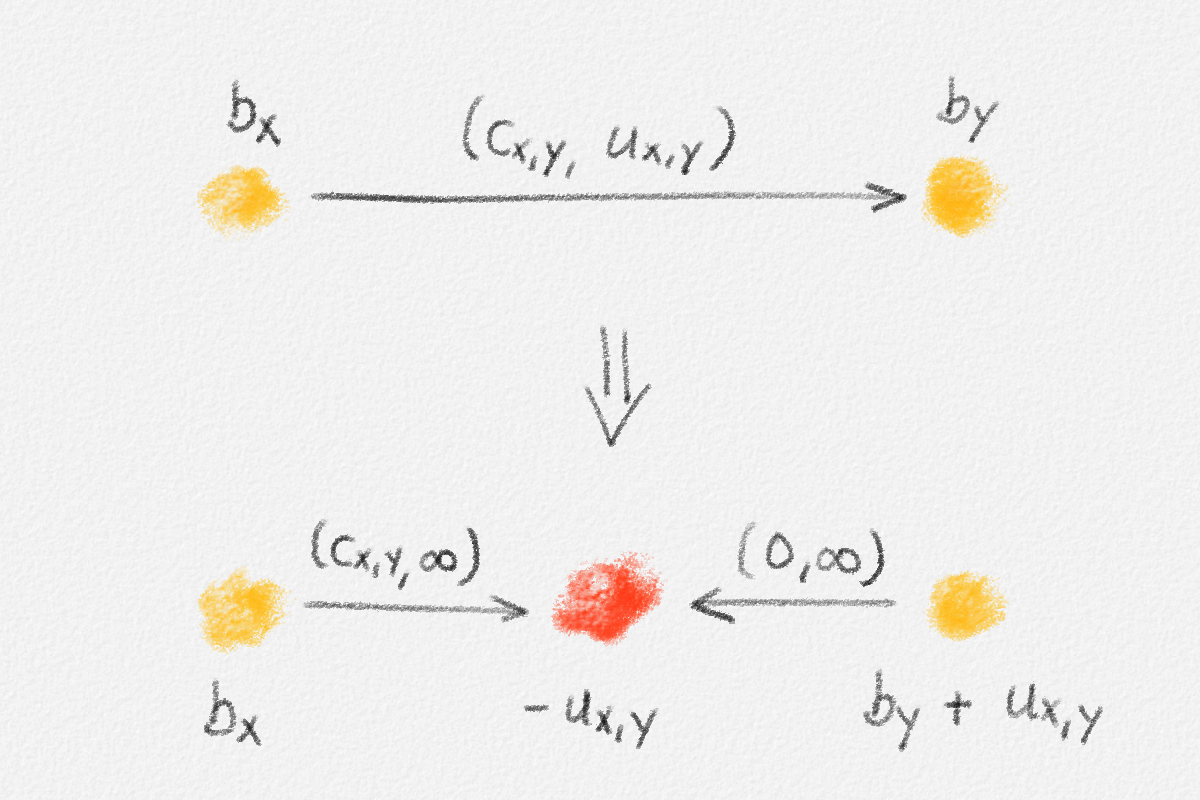
The resulting network \(H\) clearly has no edges of finite capacity. As the next two lemmas show, there exists a simple cost-preserving bijection between flows in \(G\) and flows in \(H\), so a minimum-cost flow in \(G\) can be computed by solving the minimum-cost flow problem in \(H\) instead.

For an arbitrary edge labelling \(f\) of \(G\), let \(f'\) be the corresponding edge labelling of \(H\) defined as

\[f'_{x,y} = \begin{cases} f_{x,y} & \text{if } (x, y) \in G \text{ (and thus $u_{x,y} = \infty$)}\\ f_{x,w} & \text{if } y = z_{x,w}\\ u_{w,x} - f_{w,x} & \text{if } y = z_{w,x}. \end{cases}\tag{6.9}\]

In other words, \(f\) and \(f'\) send the same amount of flow along each uncapacitated edge of \(G\); for each edge \((x, w) \in G\) with capacity \(u_{x,w} < \infty\), \(f'\) sends \(f_{x,w}\) units of flow from \(x\) to \(z_{x, w}\) and \(u_{x,w} - f_{x,w}\) units of flow from \(w\) to \(z_{x, w}\).

Lemma 6.11: \(f\) is a flow in \(G\) if and only if \(f'\) is a flow in \(H\). Both flows have the same cost.

Proof: Throughout this proof, we refer to the vertex supply functions in \(G\) and \(H\) as \(b\) and \(b'\), respectively. The capacity functions in \(G\) and \(H\) are referred to as \(u\) and \(u'\), respectively.

First we show that \(f'\) satisfies the flow conservation constraints if and only if \(f\) does.

For every vertex \(w = z_{x,y}\) in \(H\), we have

\[\sum_{v \in V} \bigl(f'_{w,v} - f'_{v,w}\bigr) = -f'_{x,w} - f'_{y,w} = -f_{x,y} - \bigl(u_{x,y} - f_{x,y}\bigr) = -u_{x,y} = b_w'.\]

Thus, no matter whether \(f\) satisfies the flow conservation constraints, \(f'\) satisfies \(w\)'s flow conservation constraint.

For every vertex \(w \in G\), let \(I_w\) be the set of vertices \(x\) such that the edge \((x,w)\) satisfies \(u_{x,w} < \infty\). Then

\[\begin{aligned} \sum_{x \in H} \bigl(f'_{w,x} - f'_{x,w}\bigr) &= \sum_{x \in V} f_{w,x} + \sum_{x \in I_w}\ \bigl(u_{x,w} - f_{x,w}\bigr) - \sum_{x \in V \setminus I_w} f_{x,w}\\ &= \sum_{x \in V} \bigl(f_{w,x} - f_{x,w}\bigr) + \sum_{x \in I_w} u_{x,w}. \end{aligned}\]

Let

\[\delta_w = \sum_{x \in V}\bigl(f_{w,x} - f_{x,w}\bigr) - b_w.\]

Then

\[\sum_{x \in H} \bigl(f'_{w,x} - f'_{x,w}\bigr) = b_w + \delta_w + \sum_{x \in I_w} u_{x,w} = b'_w + \delta_w.\]

Therefore,

\[\sum_{x \in G'} \bigl(f'_{w,x}- f'_{x,w}\bigr) = b'_w \quad \Leftrightarrow \quad \delta_w = 0 \quad \Leftrightarrow \quad \sum_{x \in V} \bigl(f_{w,x} - f_{x,w}\bigr) = b_w.\]

Thus, \(f\) satisfies the flow conservation constraints in \(G\) if and only if \(f'\) does in \(H\).

Next assume that \(f\) and \(f'\) satisfy the flow conservation constraints in \(G\) and \(H\), respectively. We prove that \(f\) satisfies the capacity constraints in \(G\) if and only if \(f'\) does in \(H\). Consider any edge \((x, y) \in G\).

If \(u_{x,y} = \infty\), then \((x, y) \in H\) and \(f'_{x,y} = f_{x,y}\), and \(u'_{x,y} = \infty\). Thus, \(f_{x,y} \le u_{x,y}\), \(f'_{x,y} \le u'_{x,y}\), and \(f_{x,y} \ge 0\) if and only if \(f'_{x,y} \ge 0\). In other words, \(f\) satisfies the capacity constraint of the edge \((x,y)\) in \(G\) if and only if \(f'\) satisfies the capacity constraint of the edge \((x,y)\) in \(H\).

If \(u_{x,y} < \infty\), then \((x, y) \notin H\) and \(H\) contains two edges \(\bigl(x, z_{x,y}\bigr)\) and \(\bigl(y, z_{x,y}\bigr)\) with \(f'_{x,z_{x,y}} = f_{x,y}\) and \(f'_{y,z_{x,y}} = u_{x,y} - f_{x,y}\). Thus,

\[0 \le f_{x,y} \le u_{x,y} \quad \Leftrightarrow \quad 0 \le f'_{x,z_{x,y}} \text{ and } 0 \le u_{x,y} - f_{x,y} = f'_{y,z_{x,y}}.\]

In other words, \(f\) satisfies the capacity constraint of the edge \((x,y)\) in \(G\) if and only if \(f'\) satisfies the capacity constraints of the two edges \(\bigl(x,z_{x,y}\bigr)\) and \(\bigl(y,z_{x,y}\bigr)\) in \(H\).

Since \(f\) satisfies both the capacity and flow conservation constraints in \(G\) if and only if \(f'\) does in \(H\), this shows that \(f\) is a flow in \(G\) if and only if \(f'\) is a flow in \(H\).

To determine the cost of \(f'\), we can divide the edges of \(H\) into two groups: For every edge \((x,y) \in G\) with \(u_{x,y} = \infty\), \(H\) also contains the edge \((x,y)\) and we have \(f'_{x,y} = f_{x,y}\) and \(c'_{x,y} = c_{x,y}\). For every edge \((x,y) \in G\) with \(u_{x,y} < \infty\), \(H\) contains the edge \(\bigl(x, z_{x,y}\bigr)\) and once again, \(f'_{x, z_{x,y}} = f_{x,y}\) and \(c'_{x, z_{x,y}} = c_{x,y}\). These are the edges in the first group \(E_1'\). We have

\[\sum_{e \in G} c_ef_e = \sum_{e \in E_1'}c'_ef'_e.\]

The second group \(E_2'\) contains all remaining edges of \(H\). Any such edge \((x,y) \in E_2'\) satisfies \(y = z_{w,x}\) for some edge \((w,x) \in G\) with \(u_{w,x} < \infty\). Thus, \(c'_{x,y} = 0\) and

\[\sum_{e \in E_2'}c'_ef'_e = 0.\]

Together, these two equalities imply that

\[\sum_{e \in H} c'_ef'_e = \sum_{e \in E_1'} c'_ef'_e + \sum_{e \in E_2'} c'_ef'_e = \sum_{e \in G} c_ef_e,\]

that is, \(f\) and \(f'\) have the same cost. ▨

By Lemma 6.11, every flow \(f\) in \(G\) has a corresponding flow \(f'\) in \(H\) of the same cost, defined by (6.9). The following observation shows that every flow \(f'\) in \(H\) corresponds to a flow in \(f\) via (6.9). Since this mapping has an obvious inverse, it is thus a bijection between flows in \(G\) and flows in \(H\). Since each flow \(f\) in \(G\) has the same cost as its corresponding flow in \(H\), it is thus also a bijection between minimum-cost flows in \(G\) and \(H\).

Observation 6.12: For every flow \(f'\) in \(H\), there exists a flow \(f\) in \(G\) such that \(f'\) is obtained from \(f\) via (6.9).

Proof: Let \(f\) be defined as

\[f_{x,y} = \begin{cases} f'_{x,y} & \text{if } u_{x,y} = \infty\\ f'_{x,z_{x,y}} & \text{if } u_{x,y} < \infty, \end{cases}\]

and let \(f''\) be the edge labelling obtained from \(f\) via (6.9). If \(u_{x,y} = \infty\), then \(f''_{x,y} = f_{x,y} = f'_{x,y}\). If \(u_{x,y} < \infty\), then \(f''_{x,z_{x,y}} = f_{x,y} = f'_{x,z_{x,y}}\) and \(f''_{y,z_{x,y}} = u_{x,y} - f_{x,y}\). Since \(f'\) satisfies flow conservation at \(z_{x,y}\), we have

\[\begin{aligned} f'_{x,z_{x,y}} + f'_{y,z_{x,y}} &= -b_{z_{x,y}}\\ f_{x,y} + f'_{y,z_{x,y}} &= u_{x,y}\\ f'_{y,z_{x,y}} &= u_{x,y} - f_{x,y} = f''_{y,z_{x,y}}. \end{aligned}\]

Thus, \(f' = f''\). By Lemma 6.11, \(f\) is a flow in \(G\) since \(f'\) is a flow in \(H\). ▨

Note that, if \(G\) has \(n\) vertices and \(m\) edges, then \(H\) has at most \(n + m\) vertices and at most \(2m\) edges. Some of the algorithms discussed in this section repeatedly compute shortest paths in a residual network, using Dijkstra's algorithm. On \(G\), this would take \(O(n \lg n + m)\) time. On \(H\), it seems to take \(O((n + m) \lg n + m) = O(m \lg n)\) time, which can be worse by a \(\lg n\) factor if \(G\) is sufficiently dense. The following exercise asks you to show that the single-source shortest paths problem in \(H\) can in fact be solved in \(O(n \lg n + m)\) time:

Exercise 6.3: Consider a graph \(G = (U \cup W, E)\) whose vertex set can be divided into two subsets \(U\) and \(W\) such that every vertex in \(W\) has exactly two neighbours, both of which are in \(U\), while the vertices in \(U\) may have an arbitrary number of neighbours, and these neighbours may be in \(U\) or \(W\). Let \(n_U = |U|\) and \(m = |E|\). Prove that the single-source shortest paths problem in \(G\) can be solved in \(O(n_U \lg n_U + m)\) time.

6.3.4. Making Edge Costs Non-Negative

Some algorithms for computing minimum-cost flows assume that all edges have non-negative costs. The final transformation we discuss here shows how to satisfy this assumption. This transformation assumes that every edge has finite capacity, which we can ensure using the transformation in Section 6.3.2. Under this assumption, we can reduce the problem of computing a minimum-cost flow in \(G\) to computing a minimum-cost flow in the following network \(H\): Let \(E^-\) be the set of all edges of \(G\) with negative costs and let \(E^+ = E \setminus E^-\). Then \(H\) has the edge set \(E^+ \cup E^-_r\), where \(E^-_r = \{ (y, x) \mid (x, y) \in E^- \}\), that is, every negative-cost edge is reversed in \(H\). Every edge \((x, y) \in E^+\) has the same cost and capacity in \(H\) as in \(G\): \(u'_{x,y} = u_{x,y}\) and \(c'_{x,y} = c_{x,y}\). Every edge \((y, x) \in E^-_r\) has capacity \(u'_{y,x} = u_{x,y}\) and cost \(c'_{y,x} = -c_{x,y}\). Thus, every edge in \(H\) has non-negative cost. Finally, the node supplies in \(H\) are defined as

\[b'_y = b_y + \sum_{(x, y) \in E^-} u_{x,y} - \sum_{(y, z) \in E^-} u_{y,z}.\]

Intuitively, \(H\) is the residual network of \(G\) when saturating all negative-cost edges of \(G\): \(H = G^f\), where

\[f_{x,y} = \begin{cases} 0 & \text{if } c_{x,y} \ge 0\\ u_{x,y} & \text{if } c_{x,y} < 0. \end{cases}\]

The following lemma establishes a bijection between flows in \(G\) and \(H\). Its corollary shows that this implies that a minimum-cost flow in \(G\) can be obtained in a straightforward manner from a minimum-cost flow in \(H\).

Lemma 6.13: Consider two edge labellings \(f\) and \(f'\) of the edges in \(G\) and \(H\), respectively, such that

\[f'_{x,y} = \begin{cases} f_{x,y} & \text{if } (x, y) \in E^+\\ u_{y,x} - f_{y,x} & \text{if } (y, x) \in E^-. \end{cases}\]

Then \(f\) is a flow in \(G\) if and only if \(f'\) is a flow in \(H\).

Proof: First consider the flow conservation constraints. \(f\) satisfies these constraints in \(G\) if and only if

\[\begin{aligned} b_x &= \sum_{y \in V} \bigl(f_{x,y} - f_{y,x}\bigr)\\ &= \sum_{\substack{y \in V\\(x, y) \in E^+}} f_{x,y} + \sum_{\substack{y \in V\\(x, y) \in E^-}} f_{x,y} - \sum_{\substack{y \in V\\(y, x) \in E^+}} f_{y,x} - \sum_{\substack{y \in V\\(y, x) \in E^-}} f_{y,x}\\ &= \sum_{\substack{y \in V\\(x, y) \in E^+}} f'_{x,y} + \sum_{\substack{y \in V\\(y, x) \in E^-_r}} \bigl(u_{x,y} - f'_{y,x}\bigr) - \sum_{\substack{y \in V\\(y, x) \in E^+}} f'_{y,x} - \sum_{\substack{y \in V\\(x, y) \in E^-_r}} \bigl(u_{y,x} - f'_{x,y}\bigr)\\ &= \sum_{y \in V} \bigl(f'_{x,y} - f'_{y,x}\bigr) + \sum_{(x, y) \in E^-} u_{x,y} - \sum_{(y, x) \in E^-} u_{y,x}, \end{aligned}\]

which is true if and only if

\[b_x - \sum_{(x, y) \in E^-} u_{x,y} + \sum_{(y, x) \in E^-} u_{y,x} = \sum_{y \in V} \bigl(f'_{x,y} - f'_{y,x}\bigr),\]

that is, if and only if

\[b'_x = \sum_{y \in V} \bigl(f'_{x,y} - f'_{y,x}\bigr).\]

Thus, \(f\) satisfies the flow conservations constraints in \(G\) if and only if \(f'\) does in \(H\).

Next consider the capacity constraints. \(f\) satisfies the capacity constraints in \(G\) if and only if, for every edge \((x, y) \in G\),

\[0 \le f_{x,y} \le u_{x,y}.\]

If \((x,y) \in E^+\), then this is true if and only if \(0 \le f'_{x,y} \le u'_{x,y}\) because \(f'_{x,y} = f_{x,y}\) and \(u'_{x,y} = u_{x,y}\).

If \((x, y) \in E^-\), then \((y, x) \in E^-_r\), \(u'_{y,x} = u_{x,y}\), and \(f'_{y,x} = u_{x,y} - f_{x,y}\). Thus, \(0 \le f_{x,y} \le u_{x,y}\) if and only if \(0 \le u_{x,y} - f_{x,y} \le u_{x,y}\), that is, if and only if \(0 \le f'_{y,x} \le u'_{y,x}\).

This shows that \(f\) satisfies the capacity constraints in \(G\) if and only if \(f'\) satisfies the capacity constraints in \(H\). ▨

Corollary 6.14: For two flows \(f\) and \(f'\) as in Lemma 6.13, \(f\) is a minimum-cost flow in \(G\) if and only if \(f'\) is a minimum-cost flow in \(H\).

Proof: Consider two flows \(f^{(1)}\) and \(f^{(2)}\) in \(G\) and their corresponding flows \(g^{(1)}\) and \(g^{(2)}\) in \(H\) as defined in Lemma 6.13. For \(i \in \{1, 2\}\), the cost of \(f^{(i)}\) is \(\sum_{e \in E} c_ef^{(i)}_e\). The cost of \(g^{(i)}\) is

\[\begin{aligned} \sum_{(x, y) \in E^+} c'_{x,y} g^{(i)}_{x,y} + \sum_{(y, x) \in E^-_r} c'_{y,x} g^{(i)}_{y,x} &= \sum_{(x, y) \in E^+} c_{x,y} f^{(i)}_{x,y} - \sum_{(x, y) \in E^-} c_{x,y} \Bigl(u_{x,y} - f^{(i)}_{x,y}\Bigr)\\ &= \sum_{e \in E} c_ef^{(i)}_e - \sum_{e \in E^-} c_eu_e. \end{aligned}\]

Thus, the cost of \(g^{(i)}\) is exactly \(\sum_{e \in E^-} c_eu_e\) lower than the cost of \(f^{(i)}\). Therefore, \(f^{(1)}\) has a lower cost than \(f^{(2)}\) if and only if \(g^{(1)}\) has a lower cost than \(g^{(2)}\), that is, the transformation in Lemma 6.13 establishes a bijection between the minimum-cost flows in \(G\) and \(H\). ▨

6.4. Negative Cycle Cancelling

The negative cycle optimality criterion of a minimum-cost flow established by Lemma 6.3 leads to our first, simple algorithm for computing a minimum-cost flow in a network.

This algorithm assumes that all edge capacities and edge costs are integers.

This integrality assumption is one we cannot eliminate using a simple transformation of the network. Thus, this algorithm really only works for integral edge capacities and edge costs.

The algorithm proceeds in two phases: In the first phase, it finds a feasible flow or decides that no such flow exists. In the case of maximum \(st\)-flows, the flow \(f\) defined as \(f_e = 0\) for all \(e \in G\) is a feasible flow, so there always exists a feasible \(st\)-flow. When looking for a minimum-cost flow, every vertex has a specific supply balance and it is not guaranteed that the edge capacities of the network allow us to send all the supply provided by supply nodes to appropriate demand nodes. Thus, there may be no feasible solution for a given instance of the minimum-cost flow problem.

If the first phase finds a feasible flow \(f\), the second phase transforms \(f\) into a minimum-cost flow. It checks whether the residual network \(G^f\) contains any negative cycle \(C\). If there is no such cycle, then \(f\) is a minimum-cost flow, by Lemma 6.3. Otherwise, the algorithm sends \(\delta\) units of flow along \(C\), where \(\delta\) is the minimum residual capacity of the edges in \(C\). The resulting flow \(f'\) is a feasible flow of lower cost than \(f\). Moreover, since sending \(\delta\) units of flow along \(C\) saturates at least one edge in \(C\), \(C\) is not a cycle in \(G^{f'}\)—\(C\) has been eliminated (or "cancelled"). This gives the algorithm its name: the negative cycle cancelling algorithm. Given the flow \(f'\), the algorithm continues to look for negative cycles in \(G^{f'}\) and cancels them until we obtain a flow whose residual network contains no such cycle.

Section 6.4.1 discusses the first phase of the algorithm, that is, how to find a feasible flow. Section 6.4.2 discusses the second phase of the algorithm. In particular, we need to figure out how to find negative cycles efficiently.

6.4.1. Finding a Feasible Flow

To find a feasible flow or decide that no such flow exists, we can use any maximum-flow algorithm: We transform \(G\) into a network \(H\) by adding two vertices \(s\) and \(t\) to \(G\). We add an edge of capacity \(b_x\) from \(s\) to every supply node \(x\) and an edge of capacity \(-b_x\) from every demand node \(x\) to \(t\). The edges of \(G\) have the same capacity in \(H\) as in \(G\).

Observation 6.15: There exists a feasible flow in \(G\) if and only if \(H\) has a maximum \(st\)-flow \(f'\) with \(F'_s = \sum_{x \in G} \max(0, b_x)\). If there exists such an \(st\)-flow in \(H\), then the flow \(f\) defined as \(f_e = f'_e\) for all \(e \in G\) is a feasible flow in \(G\).

Exercise 6.4: Prove Observation 6.15.

6.4.2. Cancelling Negative Cycles

As already said, the second phase of the negative cycle cancelling algorithm starts with the feasible flow computed in the first phase and reduces its cost by cancelling negative cycles.

Let \(f\) be the current flow. If there is no negative cycle in its residual network \(G^f\), then \(f\) is a minimum-cost flow and we return it. Otherwise, let \(C\) be a negative cycle in \(G^f\) and let

\[\delta = \min_{e \in C} u^f_e\]

be the minimum residual capacity of the edges in \(C\). Then we construct a new flow \(f'\) defined as

\[f'_{x,y} = \begin{cases} f_{x,y} + \delta & \text{if } (x, x) \in C\\ f_{x,y} - \delta & \text{if } (y, x) \in C\\ f_{x,y} & \text{otherwise.} \end{cases}\]

By Lemma 6.7, \(f'\) is indeed a flow. We replace \(f\) with \(f'\) and start another iteration. This process continues until \(G^f\) contains no negative cycle and the algorithm returns \(f\). By Lemma 6.3, \(f\) is a minimum-cost flow at this point. The three questions we need to answer are whether the algorithm terminates, how many iterations it takes to do so, and how long every iteration takes.

We focus on the last question first. Given a negative cycle \(C\) in \(G^f\), we can easily find \(\delta\) in \(O(n)\) time by inspecting every edge in \(C\), and we can compute \(f'\) from \(f\) in \(O(n)\) time by adjusting the flow along every edge of \(G\) that corresponds to an edge in \(C\). The only challenge therefore is to find \(C\) (or determine that no such cycle exists). By the following lemma, this takes \(O(nm)\) time.

Lemma 6.16: It takes \(O(nm)\) time to decide whether a network \(G\) has a negative cycle and, if so, find one.

Proof: Recall the Bellman-Ford algorithm for computing shortest paths from a vertex \(s\) to all vertices in \(G\) in the absence of negative cycles. This algorithm takes \(O(nm)\) time. It turns out that we can use the same algorithm, with minor modifications, also to detect and find negative cycles.

The Bellman-Ford algorithm initializes distance labels \(d_x\) for all vertices \(x \in G\) by setting \(d_s = 0\) and \(d_x = \infty\). It also maintains the predecessor \(p_x\) of every vertex \(x\) on the shortest path from \(s\) to \(x\) found so far. Initially, \(p_x = \textrm{NULL}\). Then the algorithm repeats the following steps \(n - 1\) times, that is, it runs for \(n - 1\) iterations:

• For every vertex \(y \in G\), set

  \[d'_y = \min\bigl(d_y, \min_{(x,y) \in G} \bigl(d_x + w_{x,y}\bigr)\bigr),\]

  where \(w_{x,y}\) is the length of the edge \((x,y)\).

• If \(d'_y < d_y\), then set \(p_y = x\), where \(x\) is any in-neighbour of \(y\) that satisfies \(d'_y = d_x + w_{x,y}\).

• Finally, set \(d_y = d'_y\) for all \(y \in G\).

In the remainder of this proof, we use \(d^{(0)}_x\) and \(p^{(0)}_x\) to refer to the initial values of \(d_x\) and \(p_x\) before the first iteration, and \(d^{(i)}_x\) and \(p^{(i)}_x\) to refer to the values of \(d_x\) and \(p_x\) at the end of the \(i\)th iteration.

To test whether \(G^f\) contains a negative cycle, we use the Bellman-Ford algorithm as follows: First we add a new vertex \(s\) to \(G^f\) along with an edge of length \(0\) from \(s\) to every vertex \(x \in G^f\). This ensures that every vertex in \(G^f\) is reachable from \(s\) and thus that it has a finite distance from \(s\). The length of every edge \(e \in G^f\) is chosen to be the same as its residual cost \(c^f_e\). Then we run the Bellman-Ford algorithm with \(s\) as the source, but we run it for one additional iteration, for \(n\) iterations in total (where \(n\) is the number of vertices including \(s\))!

The following claim shows that we can use the output of the Bellman-Ford algorithm to decide whether there exists a negative cycle in \(G^f\).

Claim 6.17: There exists a negative cycle in \(G^f\) if and only if \(d^{(n)}_x < d^{(n-1)}_x\) for some vertex \(x \in G^f\).¹

Proof: First assume that there is no negative cycle in \(G^f\). Adding \(s\) to \(G^f\) does not introduce any negative cycle because \(s\) has only out-edges. Thus, according to the correctness proof of the Bellman-Ford algorithm, \(d^{(n-1)}_x = \mathrm{dist}_{G^f}(s,x)\) for all \(x \in G^f\). Since \(\mathrm{dist}_{G^f}(s,y) \le \mathrm{dist}_{G^f}(s,x) + c^f_{x,y}\) for every edge \((x,y) \in G^f\), this implies that \(d^{(n-1)}_y \le d^{(n-1)}_x + c^f_{x,y}\) for every edge \((x,y) \in G^f\), that is,

\[d^{(n)}_y = \min\left(d^{(n-1)}_y, \min_{(x,y) \in G^f}\left(d^{(n-1)}_x + c^f_{x,y}\right)\right) = d^{(n-1)}_y \quad \forall y \in G^f.\]

Thus, there is no vertex \(y \in G^f\) with \(d^{(n)}_y < d^{(n-1)}_y\).

Conversely, assume that \(d^{(n)}_y = d^{(n-1)}_y\) for every vertex \(y \in G^f\). Then

\[d^{(n-1)}_y \le d^{(n-1)}_x + c^f_{x,y} \quad \forall (x, y) \in G^f.\]

Let \(C = \langle x_0, \ldots, x_r \rangle\) be any cycle in \(G^f\). Then

\[d^{(n-1)}_{x_r} \le d^{(n-1)}_{x_0} + \sum_{i=1}^r c^f_{x_{i-1},x_i},\]

which implies that

\[0 \le \sum_{i=1}^r c^f_{x_{i-1}, x_i} = c^f(C)\]

because \(x_0 = x_r\). Thus, there is no negative cycle in \(G^f\). ▣

After spending \(O(nm)\) time to run the Bellman-Ford algorithm, Claim 6.17 allows us to decide in \(O(n)\) time whether \(G^f\) contains a negative cycle. If there exists a negative cycle in \(G^f\), we find such a cycle as follows: We choose an arbitrary vertex \(x_0\) that satisfies \(d^{(n)}_{x_0} < d^{(n-1)}_{x_0}\) and set \(i = 0\). As long as \(p^{(n)}_{x_i} \ne s\) and \(p^{(n)}_{x_i} \notin \{x_0, \ldots, x_i\}\), we define \(x_{i+1} = p^{(n)}_{x_i}\) and increase \(i\) by one. We prove below that the situation when \(p^{(n)}_{x_i} = s\) never arises. Thus, the algorithm exits only when it determines that \(p^{(n)}_{x_i} \in \{x_0, \ldots, x_i\}\). In this case, there exists a unique index \(0 \le j \le i\) such that \(p^{(n)}_{x_i} = x_j\). We prove below that \(C = \langle x_{i+1}, x_i, \ldots, x_j \rangle\) is a negative cycle in \(G^f\). Finding \(C\) in this fashion clearly takes \(O(n)\) time: We start by marking all vertices as unexplored, marking \(x_0\) as explored, and setting \(C = \langle x_0 \rangle\). As long as \(p^{(n)}_{x_i}\) is unexplored, we prepend it to \(C\) and mark it as explored. This takes constant time, and we can do this at most \(n\) times because there are only \(n\) vertices we can add to \(C\). When \(p^{(n)}_{x_i}\) is explored, we find its occurrence \(x_j \in C\) and remove all vertices that come after \(x_j\) in \(C\) from \(C\). This clearly takes \(O(|C|) = O(n)\) time.

To prove that this procedure does indeed find a negative cycle in \(G^f\), we need the following observation, which should be obvious:

Observation 6.18: For all \(0 \le i \le n\), \(d^{(i)}_y\) is the length of a shortest walk² from \(s\) to \(y\) with at most \(i\) edges. If \(d^{(i)}_y \ne \infty\) and \(y \ne s\), then \(d^{(i)}_y = d^{(i-1)}_{p^{(i)}_y} + c^f_{p^{(i)}_y, y}\).

To complete the correctness proof of our negative cycle finding algorithm, we prove first that the termination condition \(p^{(n)}_{x_i} = s\) is never reached. Assume the contrary and consider the path \(P = \langle x_{i+1}, x_i, \ldots, x_0 \rangle\), where \(x_{i+1} = p^{(n)}_{x_i} = s\). By Observation 6.18, we have

\[\begin{aligned} d^{(n)}_{x_h} &= d^{(n-1)}_{p^{(n)}_{x_h}} + c^f_{p^{(n)}_{x_h}, x_h}\\ &= d^{(n-1)}_{x_{h+1}} + c^f_{x_{h+1}, x_h}\\ &\ge d^{(n)}_{x_{h+1}} + c^f_{x_{h+1}, x_h} \end{aligned}\]

for all \(0 \le h \le i\). Thus,

\[d^{(n)}_{x_0} \ge \sum_{h=0}^i c^f_{x_{h+1}, x_h} = c^f_P \ge d^{(n-1)}_{x_0}.\]

The last inequality follows because \(P\) visits at most \(n\) vertices and thus has at most \(n - 1\) edges and, by Observation 6.18, \(d^{(n-1)}_{x_0}\) is the length of a shortest walk from \(s\) to \(x_0\) with at most \(n - 1\) edges. However, \(x_0\) was chosen so that \(d^{(n)}_{x_0} < d^{(n-1)}_{x_0}\). We have arrived at a contradiction. Thus, when the algorithm terminates, we have \(p^{(n)}_{x_i} = x_j\) for some \(0 \le j \le i\). It remains to prove that \(C = \langle x_{i+1}, x_i, \ldots, x_j \rangle\) is a negative cycle in \(G^f\).

Since \(x_{h+1} = p^{(n)}_{x_h}\) for all \(0 \le h \le i\), \(G^f\) contains the edge \((x_{h+1}, x_h)\) for all \(0 \le h \le i\). Since \(x_{i+1} = p^{(n)}_{x_i} = x_j\), \(C\) is thus a cycle in \(G^f\). It remains to prove that its cost is negative.

Let \(m\) be the minimum index such that \(d^{(m)}_{x_h} = d^{(n)}_{x_h}\) for all \(x_h \in C\). Then there exists a vertex \(x_h \in C\) such that \(d^{(m)}_{x_h} \ne d^{(m-1)}_{x_h}\). Since \(d^{(i)}_{x_h} \le d^{(i-1)}_{x_h}\) for all \(i\), we thus have \(d^{(m)}_{x_h} < d^{(m-1)}_{x_h}\). Let us rename the vertices in \(C\) as \(C = \langle x_h = y_0, \ldots, y_{i-j-1} = x_h \rangle\). Then

\[d^{(m-1)}_{y_k} \ge d^{(m)}_{y_k} = d^{(m-1)}_{y_{k-1}} + c^f_{y_{k-1},y_k} \ge d^{(m)}_{y_{k-1}} + c^f_{y_{k-1},y_k} \quad \forall 1 \le k \le i - j - 1\]

because \(y_{k-1} = p^{(m)}_{y_k}\) for all \(1 \le k \le i - j - 1\). Thus,

\[\begin{aligned} d^{(m-1)}_{x_h} > d^{(m)}_{x_h} &\ge d^{(m-1)}_{x_h} + \sum_{k=1}^{i-j-1} c^f_{y_{k-1},y_k}\\ 0 &> \sum_{k=1}^{i-j-1} c^f_{y_{k-1},y_k} = c^f_C, \end{aligned}\]

that is, \(C\) is a negative cycle. ▨

We are ready to state the main result of this section:

Theorem 6.19: The negative cycle cancelling algorithm takes \(O\bigl(nm^2 CU\bigr)\) time to compute a minimum-cost flow in a network whose vertices have integer supply balances between \(-U\) and \(U\) and whose edges have integer capacities no greater than \(U\) and integer costs between \(-C\) and \(C\).

Proof: Finding an initial flow using any of the maximum flow algorithms from the previous chapter takes \(O\bigl(nm^2\bigr)\) time. By Lemma 6.16, finding a negative cycle takes \(O(nm)\) time and it is easy to see that updating the flow using this negative cycle also takes \(O(nm)\) time. Thus, it suffices to prove that the second phase of the algorithm runs for at most \(mCU\) iterations.

The initial flow has cost at most \(m_1CU\), where \(m_1\) is the number of edges with positive cost: Every edge carries at most \(U\) units of flow and has a cost of at most \(C\), so it contributes at most \(CU\) to the cost of the flow. By an analogous argument, the final flow has cost at least \(-m_2CU\), where \(m_2\) is the number of edges with negative cost because every edge carries at most \(U\) units of flow and has cost at least \(-C\). Now observe that sending any flow along a negative cycle in \(G^f\) strictly decreases the cost of the flow. Since the flow, and thus its cost, is integral at all times, each iteration of the second phase therefore decreases the cost of the flow by at least \(1\). Since the second phase starts with a flow of cost at most \(m_1CU\) and terminates with a flow of cost at least \(-m_2CU\), this implies that the algorithm terminates after at most \((m_1 + m_2)CU \le mCU\) iterations. ▨

6.5. Successive Shortest Paths

The strategy of the negative cycle cancelling algorithm was to compute an initial flow and then improve its cost by eliminating negative cycles until an optimal flow is obtained. The successive shortest paths algorithm takes a different approach. It starts with an optimal pseudo-flow. The algorithm then moves flow from nodes with positive excess to nodes with negative excess while maintaining optimality of the pseudo-flow until all nodes have excess \(0\). At this point, the resulting pseudo-flow is a flow and it is optimal.

As noted at the beginning of this chapter, this strategy is similar to preflow-push maximum flow algorithms. Those algorithms also started with an optimal preflow and then "drained" nodes with positive excess by pushing flow to their neighbours until the result was a flow, which was an optimal flow.

• It is far from clear what an "optimal" preflow or pseudo-flow is, given that the normal definition of an optimal solution is as a feasible solution with the best objective function value among all feasible solutions, but a preflow or pseudo-flow may not be feasible because it may violate flow conservation. Section 6.5.1 formalizes this notion of "optimality" of an infeasible solution and introduces the algorithmic paradigm on which both preflow-push algorithms and the successive shortest paths algorithm is based: the primal-dual-schema. This technique has been used to design a large number of exact and approximate optimization algorithms. In Sections 7.5.2 and 7.5.3, we discuss the Hungarian algorithm as another application of the primal-dual schema. In Chapter 12, we discuss how the primal-dual schema can be used to design approximation algorithms.

• Given the primal-dual schema, the successive shortest paths algorithm is then stated easily, and its proof of correctness and analysis are equally easy. We cover these in Section 6.5.2.

6.5.1. The Primal-Dual Schema

The right way to define what an "optimal" infeasible solution (a preflow in preflow-push algorithms, a pseudo-flow in the successive shortest paths algorithm) is to look at the problem through the lens of LP duality and complementary slackness. Both preflow-push algorithms and the successive shortest paths algorithm introduced in this section maintain a possibly infeasible primal solution—the preflow or pseudo-flow—and a feasible dual solution—a height or potential function of the vertices. At all times, the two solutions satisfy the primal complementary slackness conditions. It is in this sense that we consider the preflow or pseudo-flow to be optimal. As the algorithm progresses, it maintains primal complementary slackness while moving the primal solution towards feasibility, and it maintains that the dual solution is feasible while moving it towards optimality. At the end of the algorithm, both primal and dual solutions are feasible and satisfy complementary slackness. Thus, they are optimal solutions.

If an algorithm takes this approach of maintaining an infeasible but optimal primal solution and a feasible dual solution, and then gradually moving the primal towards feasibility while maintaining its optimality, it is said to use the primal-dual schema:

Every algorithm for some problem based on the primal-dual schema has the following characteristics:

• It maintains a primal solution of the LP formulation of the problem and a dual solution of the dual of the LP formulation.

• The dual solution is feasible at all times.

• The primal solution may be infeasible but is optimal in the sense that it satisfies some optimality criterion relative to the current dual. This criterion is often complementary slackness but can also be some problem-specific optimality criterion that is easier to work with.¹

• The algorihm iteratively updates the primal and dual solutions to move the primal towards feasibility while maintaining the optimality of the primal and the feasibility of the dual.

• Once both primal and dual are feasible, they are feasible optimal solutions because they satisfy the optimality criterion.

By the following exercise, preflow-push algorithms are indeed applications of the primal-dual schema:

Exercise 6.5: Consider the LP formulation of the maximum flow problem and its dual. Our goal is to prove the correctness of the preflow-push algorithms. Prove that a preflow \(f\) is a solution of the primal LP, and the height function \(h\) used in the algorithm is a solution of the dual LP, satisfying the following conditions:

• The initial preflow satisfies primal complementary slackness; the initial height function is a feasible dual solution.

• Every Push or Relabel operation maintains primal complementary slackness and the feasibility of the height function as a solution of the dual LP.

• When the algorithm terminates, the flow \(f\) is a feasible primal solution, the height function is a feasible dual solution, and \(f\) and \(h\) satisfy both primal and dual complementary slackness.

Next, we introduce the successive shortest paths algorithm for computing a minimum-cost flow and discuss that it is another application of the primal-dual schema.

6.5.2. The Algorithm

The successive shortest paths algorithm once again assumes that all edge capacities are integers, but it does not require the edge costs to be integers.

It does assume, however, that all edges have non-negative costs and that there exists an uncapacitated path between every pair of vertices in \(G\).

Non-negative edge costs can be guaranteed using the transformation from Section 6.3.4, if necessary after applying the transformation from Section 6.3.2 to ensure that all edge capacities are finite. Then we can apply the transformation from Section 6.3.1 to ensure the existence of an uncapacitated path between all pairs of vertices. Note, however, that if \(C\) once again refers to an upper bound on the absolute values of the edge costs, and \(U\) refers to an upper bound on the absolute values of the vertex supply balances and edge capacities, then these transformations may increase both \(C\) and \(U\) by a factor polynomial in \(n\) and \(m\).¹ The successive shortest paths algorithm maintains a pseudo-flow \(f\) and a potential function \(\pi\) that satisfy the following invariant, where \(c^\pi_e\) once again refers to the reduced cost of an edge \(e \in G^f\) with respect to the current potential function \(\pi\).

Invariant 6.20: \(c^\pi_{x,y} \ge 0\) for every edge \((x, y) \in G^f\).

By Lemma 6.2, this implies that once \(f\) is a flow, it is a minimum-cost flow. Initially, we set \(f_{x,y} = 0\) for every edge \((x, y) \in G\) and \(\pi_x = 0\) for every vertex \(x \in G\). This ensures that \(G^f = G\) at the beginning of the algorithm and, since \(c_{x,y} \ge 0\) for every edge \((x, y) \in G\), that \(c^\pi_{x,y} = c_{x,y} - \pi_x + \pi_y \ge 0\) for every edge \((x, y) \in G^f\). Thus, Invariant 6.20 holds initially.

The remainder of the algorithm proceeds in iterations. If there is no vertex in \(G^f\) with non-zero excess, then \(f\) is a flow. Thus, since \(f\) satisfies Invariant 6.20, it is a minimum-cost flow, by Lemma 6.2, and the algorithm terminates.

If there exists a vertex with non-zero excess, then observe that the existence of a vertex with positive excess implies the existence of a vertex with negative excess and vice versa (because the total excess of all vertices is zero).

Since there exists an uncapacitated path between every pair of vertices in \(G\) and every uncapacitated edge in \(G\) is easily seen to be in \(G^f\), there exists a path in \(G^f\) from every vertex with positive excess to every vertex with negative excess.

The algorithm picks an arbitrary vertex \(s\) with positive excess and finds a shortest path \(P\) in \(G^f\) to an arbitrary vertex \(t\) with negative excess, using the reduced edge costs \(c^\pi\) as the edge lengths for the shortest paths computation. Hence the algorithm's name. The proof of Lemma 6.21 below demonstrates why it is important that \(P\) is a shortest path. Since the reduced edge costs are non-negative, shortest paths from \(s\) to all vertices in \(G^f\) with respect to the reduced edge costs as edge lengths can be found in \(O(n \lg n + m)\) time using Dijkstra's algorithm.

Let

\[\delta = \min \left(e_s, -e_t, \left\{ u^f_{x,y} \mid (x, y) \in P \right\}\right)\]

and, for each vertex \(x \in V\), let \(d_x\) be the distance from \(s\) to \(x\) in \(G^f\) with respect to the reduced edge costs. Then we replace \(f\) with the pseudo-flow \(f'\) and \(\pi\) with the potential function \(\pi'\) defined as

\[f'_{x,y} = \begin{cases} f_{x,y} + \delta & \text{if } (x, y) \in P\\ f_{x,y} - \delta & \text{if } (y, x) \in P\\ f_{x,y} & \text{otherwise} \end{cases}\]

and

\[\pi'_x = \pi_x - d_x \quad \forall x \in V.\]

By Lemma 5.1, \(f'\) is indeed a pseudo-flow (because we update the flow amounts along the edges along a path in \(G^f\) in the same way the Augment procedure does). By the next lemma, replacing \(f\) and \(\pi\) with \(f'\) and \(\pi'\) maintains Invariant 6.20.

Lemma 6.21: If \(c^\pi_{x,y} \ge 0\) for every edge \((x, y) \in G^f\), then \(c^{\pi'}_{x,y} \ge 0\) for every edge \((x, y) \in G^{f'}\).

Proof: Consider any edge \((x, y) \in G^{f'}\). We distinguish two cases:

If \((x, y)\) is an edge of \(G^f\), then \(d_y \le d_x + c^\pi_{x,y}\), which implies that

\[0 \le c^\pi_{x,y} + d_x - d_y = c_{x,y} - \bigl(\pi_x - d_x\bigr) + \bigl(\pi_y - d_y\bigr) = c_{x,y} - \pi'_x + \pi'_y = c^{\pi'}_{x,y}.\]

If \((x, y)\) is not an edge of \(G^f\), then \((y, x)\) must be an edge of \(P\) because only the reversals of edges in \(P\) can be added to \(G^{f'}\). Thus,

\[d_x = d_y + c^\pi_{y,x}\]

(because \(P\) is a shortest path), that is,

\[0 = c^\pi_{y,x} + d_y - d_x = c^{\pi'}_{y,x}.\]

Since \(c^{\pi'}_{x,y} = -c^{\pi'}_{y,x}\), this shows that, once again, \(c^{\pi'}_{x,y} \ge 0\). ▨

By Lemma 6.2 and Invariant 6.20, once the successive shortest paths algorithm terminates, the current pseudo-flow \(f\) is a minimum-cost flow. It remains to bound how long it takes for the algorithm to terminate.

Theorem 6.22: The successive shortest paths algorithm takes \(O\bigl(U\bigl(n^2 \lg n + nm\bigr)\bigr)\) time to compute a minimum-cost flow in a network whose vertices have integer supply balances between \(-U\) and \(U\) and whose edges have integral capacities.

Proof: The initialization of the successive shortest paths algorithm clearly takes \(O(n + m)\) time.

Each iteration requires solving the single-source shortest paths problem in a residual network with non-negative edge lengths and updating the pseudo-flow, node potentials, residual network, and (implicitly) the reduced edge costs. This takes \(O(n \lg n + m)\) time if we use Dijkstra's algorithm to compute shortest paths. Thus, it suffices to prove that the algorithm terminates after at most \(\frac{Un}{2}\) iterations.

Since each iteration of the algorithm sends an integral positive amount of flow \(\delta\) from a node \(s\) with positive excess to a node \(t\) with negative excess, it reduces the excess of \(s\) by \(1 \le \delta \le e_s\), increases the excess of \(t\) by \(1 \le \delta \le -e_t\), and does not change the excess of any other vertex. Thus, the absolute excess \(\sum_{x \in V} |e_x|\) decreases by at least two in each iteration. The initial absolute excess is at most \(Un\) because \(|b_x| \le U\) for all \(x \in V\). Thus, it takes at most \(\frac{Un}{2}\) iterations before every node has excess \(0\). ▨

6.6. Capacity Scaling

For small integral edge costs and/or edge capacities, the negative cycle cancelling and successive shortest paths algorithms are reasonably efficient and have the benefit of being very simple. If the edge costs and edge capacities are large integers, the efficiency of these algorithms suffers. If they are real numbers, these algorithms may not terminate at all, in a manner similar to the failure of augmenting paths maximum flow algorithms to terminate unless the augmenting paths are chosen carefully.

The next algorithm we consider still assumes that the edge capacities are integers, but it exponentially increases the range of edge capacities for which the algorithm is efficient, by reducing the dependency of the running time of the algorithm on the maximum edge capacity from \(U\) to \(\lg U\). This improvement is achieved using capacity scaling, an interesting technique that has applications in many areas of algorithm design. This scaling technique can also be applied to edge costs (see e.g., Section 10.3 of Networks Flows: Theory, Algorithms, and Applications, but we do not discuss this further here.

The problem with the successive shortest paths algorithm is that it may send only a small amount of flow from a node with positive excess to a node with negative excess in each iteration. This is why it may take up to \(\frac{Un}{2}\) iterations to terminate.

The capacity scaling algorithm operates in phases and uses a strategy very similar to the successive shortest paths algorithm in each phase. However, in early phases, the algorithm guarantees that the amount of flow sent from an excess node to a deficit node in each augmentation is large. In particular, the excess node has a sufficiently large excess and the deficit node has a sufficiently large deficit. Once there is no more path from an excess node with large enough excess to a deficit node with large enough deficit, the algorithm begins the next phase, in which it is willing to consider node pairs with lower excess and deficit.

As we will see, the algorithm terminates after \(\lfloor \lg U \rfloor\) phases and performs \(O(n + m)\) augmentations in each phase. The cost of each augmentation is once again dominated by the cost of finding a shortest path from an excess node to a deficit node in (a subgraph of) the residual network and is thus \(O(n \lg n + m)\) using Dijkstra's algorithm. Thus, the capacity scaling algorithm takes \(O((n \lg n + m)(n + m)\lg U) = O\bigl(\bigl(nm \lg n + m^2\bigr) \lg U\bigr)\) time, which is better than the \(O\bigl(U\bigl(n^2 \lg n + nm\bigr)\bigr)\) time bound of the successive shortest paths algorithm as long as \(U = \omega\Bigl(\frac{m}{n}\lg\frac{m}{n}\Bigr)\). In particular, the algorithm performs better than the successive shortest paths algorithm on sparse graphs, even if the edge capacities are fairly small.

Being a variant of the successive shortest paths algorithm, the capacity scaling algorithm also assumes that there exists an uncapacitated path between every pair of vertices, and that all node supply balances and edge capacities are integers.

6.6.1. Overview of the Algorithm

As already mentioned, the capacity scaling algorithm is variant of the successive shortest paths algorithms. It maintains a pseudo-flow \(f\) and a potential function \(\pi\). When the algorithm terminates, \(f\) is a flow, and \(f\) and \(\pi\) satisfy the reduced cost optimality criterion. Thus, \(f\) is a minimum-cost flow at this point.

Initialization

The initialization of the algorithm is the same as for the successive shortest paths algorithm: We set \(f_e = 0\) for every edge \(e \in G\), and we set \(\pi_x = 0\) for every vertex \(x \in G\). As discussed in Section 6.5, this ensures that \(f\) and \(\pi\) satisfy the reduced cost optimality criterion, but \(f\) is not a feasibly flow unless we have no supply vertices and no demand vertices.

Finding a Feasible Flow

Also as in the successive shortest paths algorithm, we now repeatedly update \(f\) and \(\pi\) until \(f\) is a feasible flow, while ensuring that \(f\) and \(\pi\) continue to satisfy reduced cost optimality. The manner in which we perform these updates is where the capacity scaling algorithm differs from the successive shortest paths algorithm.

The updates of \(f\) and \(\pi\) are organized into phases. Each phase has an associated parameter \(\Delta\). In this phase, we only perform flow augmentations that send at least \(\Delta\) units of flow from an excess vertex to a deficit vertex. Given this dependence of the phase on \(\Delta\), we call this phase the \(\Delta\)-phase.

In the first phase, we set \(\Delta = 2^{\lfloor \lg U\rfloor}\). In each subsequent phase, we halve \(\Delta\) until \(\Delta = 1\) in the final phase. Thus, there are \(\lfloor \lg U \rfloor\) phases.

The \(\Delta\)-Phase

The \(\Delta\)-phase of the algorithm performs only flow augmentations that send at least \(\Delta\) units of flow from an excess vertex to a deficit vertex. To find paths along which we can send at least \(\Delta\) units of flow, the \(\Delta\)-phase works with a subgraph \(G^{f,\Delta} = \bigl(V, E^{f,\Delta}\bigr)\) of the residual network \(G^f = \bigl(V, E^f\bigr)\), where

\[E^{f,\Delta} = \bigl\{e \in E^f \mid u^f_e \ge \Delta\bigr\}.\]

We call \(G^{f,\Delta}\), the \(\Delta\)-residual network.

As long as there exists an excess vertex with excess at least \(\Delta\) and a deficit vertex with deficit at least \(\Delta\), we pick an arbitrary excess vertex \(s\) with excess at least \(\Delta\) and an arbitrary deficit vertex \(t\) with deficit at least \(\Delta\), we find a shortest path \(P\) from \(s\) to \(t\) in \(G^{f,\Delta}\), and then we send \(\delta\) units of flow from \(s\) to \(t\), where

\[\delta = \min\bigl(\bigl\{e_s, -e_t\bigr\} \cup \bigl\{c^f_e \mid e \in P\bigr\}\bigr).\]

Since \(P\) is a path in \(G^{f,\Delta}\), we have \(\delta \ge \Delta\), that is, we do indeed send at least \(\Delta\) units of flow from \(s\) to \(t\).

Sending \(\delta\) units of flow along \(P\) means that we replace \(f\) with the flow \(f'\) defined as

\[f'_{x,y} = \begin{cases} f_{x,y} + \delta & \text{if } (x, y) \in P\\ f_{x,y} - \delta & \text{if } (y, x) \in P\\ f_{x,y} & \text{otherwise.} \end{cases}\]

By Lemma 5.1, \(f'\) is once again a pseudo-flow in \(G\).

We also replace the potential function \(\pi\) with a new potential function \(pi'\) defined as

\[\pi'_x = \pi_x - d_x,\]

where \(d_x\) is the distance from \(s\) to \(x\) in \(G^{f,\Delta}\), which we compute as part of finding a shortest path from \(s\) to \(t\) in \(G^{f,\Delta}\).

Once again, this is exactly the same strategy used by the successive shortest paths algorithm. An important difference, one with implications we need to address, is that \(P\) is a shortest path in \(G^{f,\Delta}\), not in \(G^f\). There may exist a shorter path from \(s\) to \(t\) in \(G^f\), but it includes edges whose residual capacity is less than \(\Delta\). Similarly, the distance \(d_x\) subtracted from \(\pi_x\) to obtain \(\pi'_x\) for every vertex is the distance from \(s\) to \(x\) in \(G^{f,\Delta}\), not in \(G^f\).

Also as in the successive shortest paths algorithm, a path \(P\) from \(s\) to \(t\) in \(G^{f,\Delta}\) always exists because \(G\) contains an uncapacitated path from \(s\) to \(t\) and this path is then also part of \(G^{f,\Delta}\).

The \(\Delta\)-phase continues picking pairs of vertices \((s, t)\) such that \(s\) is an excess vertex with excess at least \(\Delta\) and \(t\) is a deficit vertex with deficit at least \(\Delta\) and sending flow from \(s\) to \(t\) along a shortest path in \(G^{f,\Delta}\) for each such pair, until there are either no more excess vertices with excess at least \(\Delta\) or no more deficit vertices with deficit at least \(\Delta\), possibly both.

Once we run out of excess vertices with excess at least \(\Delta\) or out of deficit vertices with deficit at least \(\Delta\), the \(\Delta\)-phase ends. If \(\Delta = 1\), then this is the last phase of the algorithm, and the algorithm returns the pseudo-flow \(f\) obtained at the end of the \(\Delta\)-phase. If \(\Delta > 1\), then we set \(\Delta = \frac{\Delta}{2}\) and start the next phase.

6.6.2. Correctness of the Algorithm

I mentioned that the fact that the capacity scaling algorithm uses shortest paths is \(G^{f,\Delta}\) to update the current pseudo-flow during the \(\Delta\)-phase, and that the potential function \(\pi\) is updated using distances in \(G^{f,\Delta}\) has important implications. In a nutshell, it means that the capacity scaling algorithm does not maintain reduced cost optimality.

In this section, we state a weaker form of reduced cost optimality that the algorithm does maintain, as well a second invariant. We will argue that this weaker reduced cost optimality condition is the same as reduced cost optimality in the final phase of the algorithm, and that the second invariant implies that at the end of the final phase—the \(1\)-phase—there are no excess vertices and no deficit vertices left. Thus, we obtain a feasible flow that satisfies reduced cost optimality at the end of the last phase. By Lemma 6.2, this implies that the flow returned by the algorithm is a minimum-cost flow.

The weaker form of reduced cost optimality maintained during the \(\Delta\)-phase is

Invariant 6.23: For every edge \(e \in G^{f,\Delta}\), \(c^\pi_e \ge 0\).

The difference to Invariant 6.20 is that we provide no guarantee that any edge \(e \in G^f\) that is not in \(G^{f,\Delta}\) (any edge with residual capacity less than \(\Delta\)) satisfies \(c^\pi_e \ge 0\).

The other invariant the algorithm maintains is

Invariant 6.24: At the beginning of the \(\Delta\)-phase, every vertex has excess less than \(2\Delta\) or every vertex has excess greater than \(-2\Delta\). At the end of the \(\Delta\)-phase, every vertex has excess less than \(\Delta\) or every vertex has excess greater than \(-\Delta\).

As the next lemma shows, these two invariants imply that the algorithm computes a minimum-cost flow:

Lemma 6.25: At the end of the \(1\)-phase (the last phase) of the capacity scaling algorithm, \(f\) is a minimum-cost flow.

Proof: By Invariant 6.24, every vertex has excess less than \(1\) or every vertex has excess greater than \(-1\) at the end of the \(1\)-phase. Since the node supply balances and edge capacities are integral, the node excesses are also integral at all times. Thus, this implies that every vertex has non-positive excess or every vertex has non-negative excess.

Since \(\sum_{x \in G} b_x = 0\) (the total supply of all supply nodes matches the total demand of all demand nodes), we also have \(\sum_{x \in G^f} e_x = 0\). Thus, if all vertices have non-positive excess or all vertices have non-negative excess, we must have that all node excesses are \(0\) and \(f\) satisfies flow conservation. Since the algorithm ensures that \(f\) is a pseudo-flow, \(f\) also satisfies the capacity constraints and is thus a flow.

To see that \(f\) is a minimum-cost flow, observe once again that all edges in \(G^f\) have integral residual capacities because the edges of \(G\) have integral capacities and therefore, \(f\) is integral. Thus, any edge in \(G^f\) has residual capacity at least \(1\) and belongs to \(G^{f,1}\): \(G^{f,1} = G^f\). By Invariant 6.23, this implies that \(c^\pi_e \ge 0\) for every edge \(e \in G^f\), and \(f\) is a minimum-cost flow, by Lemma 6.2. ▨

It remains to prove that the capacity scaling algorithm does indeed maintain Invariants 6.23 and 6.24.

6.6.2.1. Maintenance of Bounded Excesses

That the algorithm maintains Invariant 6.24 is easy to see:

At the beginning of the algorithm, we set \(f_e = 0\) for every edge \(e \in G\) and \(\pi_x = 0\) for every vertex \(x \in G\), just as in the successive shortest paths algorithm. Thus, every vertex has excess \(e_x = b_x \in [-U, U]\). Since \(\Delta = 2^{\lfloor \lg U\rfloor}\) in the first phase, we have \(U < 2\Delta\), that is, every vertex has excess strictly between \(-2\Delta\) and \(2\Delta\), and Invariant 6.24 holds at the beginning of the first phase.

Each \(\Delta\)-phase continues until there is either no excess vertex with excess at least \(\Delta\) or there is no deficit vertex with deficit at least \(\Delta\) (excess at most \(-\Delta\)). This explicitly ensures that Invariant 6.24 holds at the end of the \(\Delta\)-phase and thus also at the beginning of the \(\frac{\Delta}{2}\)-phase if \(\Delta > 1\).

6.6.2.2. Maintenance of Non-Negative Residual Costs

To ensure that the algorithm maintains Invariant 6.23, we need to fill in one more step of the algorithm. Without it, Invariant 6.23 does not hold!

I already pointed out the difference between the reduced cost optimality invariant maintained by the successive shortest paths algorithm (Invariant 6.20) and the weaker Invariant 6.23: Invariant 6.23 does not guarantee non-negative reduced costs for the edges of \(G^f\) that are not in \(G^{f,\Delta}\). When transitioning from the \(\Delta\)-phase to the \(\frac{\Delta}{2}\)-phase, note that \(G^{f,\Delta/2}\) may include some edges of \(G^f\) that are not in \(G^{f,\Delta}\): These are all the edges with residual capacities between \(\frac{\Delta}{2}\) and \(\Delta\). Thus, even though Invariant 6.23 holds for \(G^{f,\Delta}\) at the end of the \(\Delta\)-phase, it is not guaranteed to hold for \(G^{f,\Delta/2}\) at the beginning of the \(\frac{\Delta}{2}\)-phase.

We begin by arguing that the invariant does hold at the beginning of the first phase, and we show how we can restore the invariant at the beginning of every subsequent phase. We conclude the discussion in this section by showing that once Invariant 6.23 holds, the updates to \(f\) and \(\pi\) performed during the \(\Delta\)-phase do not invalidate the invariant. Thus, Invariant 6.23 is indeed maintained throughout the \(\Delta\)-phase.

The Beginning of the First Phase

In the analysis of the successive shortest paths algorithm, we observed that setting \(f_e = 0\) for every edge \(e \in G\) and \(\pi_x = 0\) for every vertex \(x \in G\) ensures that \(c^\pi_e \ge 0\) for every edge \(e \in G^f\). Since \(G^{f,\Delta} \subseteq G^f\), this shows that Invariant 6.23 holds at the beginning of the first phase of the capacity scaling algorithm.

Initialization of Any \(\boldsymbol{\Delta}\)-Phase Other Than the First Phase

To ensure that all edges in \(G^{f,\Delta}\) satisfy \(c^\pi_e \ge 0\), that is, that Invariant 6.23 holds at the beginning of the \(\Delta\)-phase, we use the same trick we used in Section 6.3.4 to ensure that all edges in \(G\) have non-negative costs: We saturate all edges with negative cost.

Specifically, we replace \(f\) with the pseudo-flow \(f'\) defined as

\[f'_{x,y} = \begin{cases} 0 & \text{if } (y,x) \in G^{f,\Delta} \text{ and } c^\pi_{y,x} < 0\\ u_{x,y} & \text{if } (x,y) \in G^{f,\Delta} \text{ and } c^\pi_{x,y} < 0\\ f_{x,y} & \text{otherwise} \end{cases}\]

and we leave the potential function \(\pi\) unchanged.

Note that \(f'\) is well defined, that is, that every edge \((x,y) \in G\) satisfies \(f'_{x,y} < \infty\). Indeed, every edge \((x,y) \in G\) satisfies \(f_{x,y} < \infty\). In the first and last cases, we set \(f'_{x,y} = 0\) or \(f'_{x,y} = f_{x,y}\), so \(f'_{x,y}\) is finite in these cases. In the second case, we can have \(f'_{x,y} = \infty\) only if \(u_{x,y} = \infty\). However, if \(u_{x,y} = \infty\), then \(u^f_{x,y} = \infty \ge 2\Delta\), that is, \((x,y) \in G_{f,2\Delta}\) and, by Invariant 6.23, we have \(c^\pi_{x,y} \ge 0\) at the end of the \(2\Delta\)-phase. Thus, the second case can apply only to capacitated edges and \(f'_{x,y} < \infty\) in this case as well.

Since \(f\) is a pseudo-flow at the end of the \(2\Delta\)-phase, \(f'\) is clearly also a pseudo-flow. The next lemma shows that \(f'\) and \(\pi\) satisfy Invariant 6.23, that is, replacing \(f\) with \(f'\) ensures that Invariant 6.23 holds at the beginning of the \(\Delta\)-phase.

Lemma 6.26: \(c^\pi_e \ge 0\) for every edge \(e \in G^{f',\Delta}\).

Proof: Assume for the sake of contradiction that \(G^{f',\Delta}\) contains an edge \((x,y)\) that satisfies \(c^\pi_{x,y} < 0\).

If \((x,y) \in G\), then \(f'_{x,y} < f_{x,y}\) only if \((y,x) \in G^{f,\Delta}\) and \(c^\pi_{y,x} < 0\). Since \(c^\pi_{x,y} = -c^\pi_{y,x}\), this immediately implies that \(c^\pi_{x,y} > 0\), a contradiction. Thus, if \((x,y) \in G\), we have \(f'_{x,y} \ge f_{x,y}\) and, thus, \(u^f_{x,y} = u_{x,y} - f_{x,y} \ge u_{x,y} - f'_{x,y} = u^{f'}_{x,y} \ge \Delta\), that is, \((x,y) \in G^{f,\Delta}\). Since \(c^\pi_{x,y} < 0\), this implies that \(f'_{x,y} = u_{x,y}\), so \(u^{f'}_{x,y} = 0\) and \((x,y) \notin G^{f',\Delta}\), again a contradiction.

If \((y,x) \in G\), then \(f'_{y,x} > f_{y,x}\) only if \((y,x) \in G^{f,\Delta}\) and \(c^\pi_{y,x} < 0\). Once again, this immediately implies that \(c^\pi_{x,y} > 0\), a contradiction. Thus, if \((y,x) \in G\), we have \(f'_{y,x} \le f_{y,x}\) and, thus, \(u^f_{x,y} = f_{y,x} \ge f'_{y,x} = u^{f'}_{x,y} \ge \Delta\), that is, \((x,y) \in G^{f,\Delta}\). Since \(c^\pi_{x,y} < 0\), this implies that \(f'_{y,x} = 0\), so \(u^{f'}_{x,y} = 0\) and \((x,y) \notin G^{f',\Delta}\), again a contradiction. ▨

Updates of \(\boldsymbol{f}\) and \(\boldsymbol{\pi}\) During the \(\boldsymbol{\Delta}\)-Phase

As we have just shown, after the initialization of the \(\Delta\)-phase, Invariant 6.23 holds. The remainder of the \(\Delta\)-phase repeatedly computes the distances of all vertices in \(G^{f,\Delta}\) from some excess vertex \(s\) with excess at least \(\Delta\) and sends flow along a shortest path in \(G^{f,\Delta}\) from \(s\) to some deficit vertex \(t\) with deficit at least \(\Delta\).

This is exactly what the successive shortest paths algorithm does in each iteration, only it uses distances and shortest paths in \(G^f\). By replacing \(G^f\) with \(G^{f,\Delta}\) in the proof of Lemma 6.21, we immediately obtain the following lemma:

Lemma 6.27: If \(c^\pi_{x,y} \ge 0\) for every edge \((x,y) \in G^{f,\Delta}\), then \(c^{\pi'}_{x,y} \ge 0\) for every edge \((x,y) \in G^{f',\Delta}\).

Thus, the \(\Delta\)-phase maintains Invariant 6.23.

6.6.3. Running Time Analysis

As already observed, the capacity scaling algorithm runs for \(\lfloor\lg U\rfloor\) phases. The initialization of each phase is easily seen to take \(O(n + m)\) time: The first phase simply sets every vertex's potential to \(\pi_x = 0\) and every edge's flow to \(f_e = 0\). In any subsequent phase, the initialization does not alter node potentials and updates the flow of every edge based on its current flow and on the potentials of its endpoints. Thus, the initialization of all phases takes \(O((n + m)\lg U)\) time in total.

As in the successive shortest paths algorithm, the cost of each individual flow augmentation is dominated by the cost of computing the distance labels and finding the shortest path along which to move flow from an excess node to a deficit node. Since we use Dijkstra's algorithm to do this, this takes \(O(n \lg n + m)\) time. Next we prove that each phase performs \(O(n + m)\) flow augmentations. Thus, we perform \(O((n + m)\lg U)\) flow augmentations in total, at a total cost of \(O\bigl(\bigl(n^2\lg n + nm\bigr)\lg U\bigr)\). The running time of the algorithm is thus \(O\bigl(\bigl(n^2\lg n + nm\bigr)\lg U\bigr)\).

Lemma 6.28: Each phase of the capacity scaling algorithm performs less than \(n + 2m\) flow augmentations.

Proof: By Invariant 6.24, we have only vertices with excess less than \(2\Delta\) or only vertices with excess greater than \(-2\Delta\) at the beginning of the \(\Delta\)-phase. Since the total excess of all excess vertices equals the total deficit of all deficit vertices, this implies that

\[e_G = \sum_{x \in G} |e_x| = \sum_{\substack{x \in G\\e_x > 0}}e_x - \sum_{\substack{x \in G\\e_x < 0}}e_x < 2\Delta n.\]

The initialization of the \(\Delta\)-phase may update \(f\) to ensure that all edges in \(G^{f,\Delta}\) have non-negative reduced costs and may therefore alter the excesses of the endpoints of the affected edges. So let \(f'\) be the flow with which the initialization of the \(\Delta\)-phase replaces \(f\), and consider any edge \((x,y) \in G\). If \(f'_{x,y} \ne f_{x,y}\), then either \((x,y) \in G^{f,\Delta}\) and \(c^\pi_{x,y} < 0\) or \((y,x) \in G^{f,\Delta}\) and \(c^\pi_{y,x} < 0\).

In the former case, \((x,y) \notin G^{f,2\Delta}\) because \(c^\pi_{w,z} \ge 0\) for every edge \((w,z) \in G^{f,2\Delta}\) at the beginning of the \(\Delta\)-phase, by Invariant 6.23. Thus, \(u_{x,y} - f_{x,y} = u^f_{x,y} < 2\Delta\) and setting \(f'_{x,y} = u_{x,y}\) ensures that \(f'_{x,y} - f_{x,y} < 2\Delta\). Replacing \(f_{x,y}\) with \(f'_{x,y}\) thus changes each of \(e_x\) and \(e_y\) by less than \(2\Delta\) and, thus, \(e_G\) by less than \(4\Delta\).

In the latter case, \((y,x) \notin G^{f,2\Delta}\), again because \(c^\pi_{w,z} \ge 0\) for every edge \((w,z) \in G^{f,2\Delta}\) at the beginning of the \(\Delta\)-phase. Thus, \(f_{x,y} = u^f_{y,x} < 2\Delta\) and setting \(f'_{x,y} = 0\) ensures that \(f_{x,y} - f'_{x,y} < 2\Delta\). Replacing \(f_{x,y}\) with \(f'_{x,y}\) therefore changes \(e_G\) by less than \(4\Delta\) once again.

Since we observed that \(e_G < 2\Delta n\) at the beginning of the \(\Delta\)-phase and there are \(m\) edges in \(G\) to which the initialization of the \(\Delta\)-phase may assign a flow \(f'_{x,y} \ne f_{x,y}\), we thus have \(e_G < 2\Delta n + 4\Delta m\) immediately after the initialization of the \(\Delta\)-phase.

Every flow augmentation in the \(\Delta\)-phase moves \(\delta \ge \Delta\) units of flow from an excess node \(s\) with \(e_s \ge \delta\) to a deficit node \(t\) with excess \(e_t \le -\delta\). Thus, it decreases \(e_G\) by \(2\delta \ge 2\Delta\). Since \(e_G < 2\Delta n + 4\Delta m\) after the initialization of the \(\Delta\)-phase, we therefore have \(e_G < 0\) after at most \(\frac{2\Delta n + 4\Delta m}{2\Delta} = n + 2m\) flow augmentations. Since \(e_G\) is easily seen to be non-negative at all times, this shows that each phase of the capacity scaling algorithm performs less than \(n + 2m\) flow augmentations. ▨

We have shown the following theorem:

Theorem 6.29: The capacity scaling algorithm takes \(O\bigl(\bigl(n^2 \lg n + nm\bigr)\lg U\bigr)\) time to compute a minimum-cost flow in a network whose vertices have integer supply balances between \(-U\) and \(U\) and whose edges have integral capacities.

Compare the capacity scaling algorithm to the successive shortest paths algorithm. The capacity scaling algorithm has to deal with some wrinkles when transitioning from one phase to the next because each phase ignores edges in the residual network with two low residual capacity. Beyond this minor complication, both algorithms are the same: they turn a pseudo-flow into a minimum-cost flow by repeatedly moving flow from excess nodes to deficit nodes. By restricting attention to node pairs with high excess and high deficit, and to paths between them with high residual capacity, at least initially, the capacity scaling algorithm is able to reduce the total number of flow augmentations to \(O((n + m)\lg U)\) whereas the successive shortest paths algorithm may perform \(O(nU)\) flow augmentations. This reduction in the number of flow augmentations is why the capacity scaling algorithm is faster than the successive shortest paths algorithm.

The scaling idea used in this section can also be applied to the edge costs instead of the edge capacities and even to both the edge costs and edge capacities. The cost scaling algorithm achieves a running time of \(O\bigl(n^3 \lg C\bigr)\), which is independent of the edge capacities and, assuming the graph is sufficiently dense and the edge costs are not too large, is faster than the capacity scaling algorithm. The double scaling algorithm, which applies scaling to both edge costs and edge capacities achieves a running time of \(O(nm \lg U \lg (nC))\), which is only little more than running Bellman-Ford's algorithm as long as the edge costs and capacities are polynomial in \(n\). For the details of these algorithm, see for example Sections 10.3 and 10.4 in Network Flows: Theory, Algorithms, and Applications. Instead of exploring these algorithms here, the remainder of this chapter focuses on minimum-cost flow algorithms whose running time is completely independent of the edge capacities and of the edge costs. These algorithms have the added benefit that they work for arbitrary real-valued edge costs and edge capacities. The next section shows how to obtain such an algorithm based on negative cycle cancelling, simply by choosing the negative cycles to cancel a little more carefully. Then we return to capacity scaling algorithms and show how to turn the \(\log U\) term in the running time of the algorithm we just discussed into a polylogarithmic term in \(n\). Note, however, that the independence of these algorithms from \(C\) and \(U\) is bought at the price of a substantially worse dependence on \(n\) and \(m\), and these algorithms are significantly more complicated. Thus, as long as the capacities or costs are integers and aren't astronomical, the algorithms discussed so far are almost always the better choice in practice.

6.7. Minimum Mean Cycle Cancelling*

The minimum mean cycle cancelling algorithm is easy to describe: Recall the negative cycle cancelling algorithm from Section 6.4.

Let the mean cost of a cycle \(C\) in \(G^f\) be defined as

\[\mu_C = \sum_{e \in C} \frac{c^f_e}{|C|},\]

that is, \(\mu_C\) is equal to the average residual cost of the edges in \(C\).

Let

\[\mu^*_f = \min_C \mu_C,\]

where the minimum is taken over all cycles in \(G^f\).

We call a cycle \(C\) that satisfies \(\mu_C = \mu^*_f\) a minimum mean cost cycle in \(G^f\).

The only change we make to turn the negative cycle cancelling algorithm into the minimum mean cycle cancelling algorithm is to choose the cycle to cancel in each iteration to be a minimum mean cost cycle.

Note that the mean cost of a cycle is negative if and only if the cycle is a negative cycle. Thus, if \(\mu^*_f \ge 0\), then \(G^f\) has no negative cycle, which implies that \(f\) is a minimum-cost flow, by Lemma 6.3. Just as the negative cycle cancelling algorithm, the algorithm terminates in this case.

If \(\mu^*_f < 0\), we find a minimum mean cost cycle \(C\) and push flow along \(C\) as in the standard negative cycle cancelling algorithm and then start another iteration. Quite surprisingly, this strategy of picking a negative cycle to cancel is sufficient to obtain a running time independent of the edge costs and capacities. While this description of the minimum mean cycle cancelling algorithm is simple, proving that it achieves a running time independent of the edge capacities and edge costs requires some effort, as we will see.

As in Sections 6.5 and 6.6, we assume that there exists an uncapacitated path between every pair of vertices in \(G\).

6.7.1. Finding a Minimum Mean Cost Cycle

First, let us figure out how to find a minimum mean cost cycle. We break the algorithm for finding a minimum mean cost cycle into two parts. First we show that \(\mu^*_f\) can be computed in \(O(nm)\) time, again using a variation of the Bellman-Ford algorithm. Then we prove that we can find a cycle of mean cost \(\mu^*_f\) in \(O\bigl(n^2\bigr)\) additional time. Together, these two claims prove

Lemma 6.30: It takes \(O(nm)\) time to find a minimum mean cost cycle \(C\) in \(G^f\).

6.7.1.1. Computing \(\boldsymbol{\mu^*_f}\)

To compute \(\mu^*_f\), we choose an arbitrary vertex \(s\) as the source and compute distance labels \(\ell^{(0)}_x, \ldots, \ell^{(n)}_x\) for all vertices \(x \in V\). We initialize \(\ell^{(0)}_s = 0\) and \(\ell^{(0)}_x = \infty\) for all \(x \ne s\) as in the Bellman-Ford algorithm. Then we run the algorithm for \(n\) iterations. The \(i\)th iteration computes \(\ell^{(i)}_x\) for all \(x \in V\). In contrast to the Bellman-Ford algorithm, which sets

\[d^{(i)}_y = \min\left(d^{(i-1)}_y, \min_{(x,y) \in E} \left(d^{(i-1)}_x + c^f_{x,y}\right)\right),\tag{6.10}\]

we define

\[\ell^{(i)}_y = \min_{(x,y) \in E} \left(\ell^{(i-1)}_x + c^f_{x,y}\right).\]

Thus, \(\ell^{(i)}_x\) is the length of a shortest walk from \(s\) to \(x\) with exactly \(i\) edges, whereas the distance label \(d^{(i)}_x\) computed by the Bellman-Ford algorithm is the length of a shortest walk from \(s\) to \(x\) with at most \(i\) edges. The vertex labellings \(\ell^{(0)}, \ldots, \ell^{(n)}\) can clearly be computed in \(O(nm)\) time. The following lemma provides the means to compute \(\mu^*_f\) from \(\ell^{(0)}, \ldots, \ell^{(n)}\) in \(O\bigl(n^2\bigr)\) time. Thus, \(\mu^*_f\) can be computed in \(O(nm)\) time in total.

Lemma 6.31:

\[\mu^*_f = \min_{x \in V} \max_{0 \le i \le n - 1} \frac{\ell^{(n)}_x - \ell^{(i)}_x}{n - i}.\tag{6.11}\]

Proof: We consider two cases:

\(\boldsymbol{\mu^*_f = 0}\): Under this assumption, there is no negative-cost cycle in \(G^f\). Thus, every vertex \(x\) has a well-defined distance \(d_x\) from \(s\). Let \(d^{(0)}, \ldots, d^{(n)}\) be the distance labellings the Bellman-Ford algorithm would have produced using the equalities (6.10). Then \(d^{(0)}_x \ge \cdots \ge d^{(n)}_x = d_x\) and \(\ell^{(i)}_x \ge d^{(i)}_x\) for all \(x \in V\) and all \(0 \le i \le n\). In particular, \(\ell^{(i)}_x \ge d_x\) for all \(x \in V\) and all \(0 \le i \le n\).

Claim 6.32: For every vertex \(x \in V\), \(\displaystyle\max_{0 \le i \le n-1}\frac{\ell^{(n)}_x - \ell^{(i)}_x}{n - i} \ge 0\).

Claim 6.33: There exists a vertex \(x \in V\) that satisfies \(\displaystyle\max_{0 \le i \le n-1}\frac{\ell^{(n)}_x - \ell^{(i)}_x}{n - i} \le 0\).

These two claims imply that

\[\min_{x \in V}\max_{0 \le i \le n-1}\frac{\ell^{(n)}_x - \ell^{(i)}_x}{n - i} = 0 = \mu^*_f,\]

that is, the lemma holds in the case when \(\mu^*_f = 0\).

Proof of Claim 6.32: Consider an arbitrary vertex \(x \in V\), let \(P\) be a shortest path from \(s\) to \(x\), and let \(k\) be the number of edges in \(P\). Then \(P\) is a walk from \(s\) to \(x\) with \(k\) edges and of length \(d_x\). Thus, \(\ell^{(k)}_x \le d_x\). Since \(\ell^{(n)}_x \ge d_x\), this implies that \(\ell^{(n)}_x \ge \ell^{(k)}_x\) and thus

\[\max_{0 \le i \le n-1} \frac{\ell^{(n)}_x - \ell^{(i)}_x}{n - i} \ge \frac{\ell^{(n)}_x - \ell^{(k)}_x}{n - k} \ge 0.\ \text{▣}\]

Proof of Claim 6.33: Since \(G^f\) is strongly connected, it contains at least one cycle. Since \(\mu^*_f = 0\), there must exist such a cycle \(C = \langle x_0, \ldots, x_t \rangle\) of cost \(c^f_C = 0\). Let \(P\) be a shortest path from \(s\) to \(x_0\), and let \(k\) be the number of edges in \(P\). By the same argument as in the previous paragraph, \(\ell^{(k)}_{x_0} \le d_{x_0}\). Thus,

\[\ell^{(k+1)}_{x_1} \le \ell^{(k)}_{x_0} + c^f_{x_0,x_1} \le d_{x_0} + c^f_{x_0, x_1}\]

and, inductively,

\[\ell^{(k+h)}_{x_{h \bmod t}} \le d_{x_0} + \sum_{j=1}^h c^f_{x_{j-1}, x_j} \quad \forall 0 \le h \le n - k.\]

For \(h = n - k\) and \(z = x_{(n - k) \bmod t}\), this gives

\[\ell^{(n)}_z \le d_{x_0} + \sum_{j=1}^{n-k} c^f_{x_{j-1}, x_j}.\]

To complete the proof of Claim 6.33, we prove that

\[d_z = d_{x_0} + \sum_{j=1}^{n-k} c^f_{x_{j-1}, x_j}.\tag{6.12}\]

This implies that \(\ell^{(n)}_z \le d_z\).¹ Since \(\ell^{(i)}_z \ge d_z\) for all \(0 \le i \le n\), we thus have

\[\frac{\ell^{(n)}_z - \ell^{(i)}_z}{n - i} \le 0 \quad \forall 0 \le i \le n - 1\]

and, thus,

\[\max_{0 \le i \le n - 1} \frac{\ell^{(n)}_z - \ell^{(i)}_z}{n - i} \le 0.\]

The distance labelling \(d\) satisfies the condition that \(d_y \le d_x + c^f_{x,y}\) for every edge \((x, y) \in G^f\). Thus, if we choose a potential function \(\pi\) defined as \(\pi_x= -d_x\) for every vertex \(x \in V\), then we obtain a reduced cost function \(c^\pi\) that satisfies

\[c^\pi_{x,y} = c^f_{x,y} - \pi_x + \pi_y = c^f_{x,y} + d_x - d_y \ge 0 \quad \forall (x,y) \in G^f.\]

The reduced cost of the cycle \(C\) is

\[c^\pi_C = \sum_{j=1}^t c^\pi_{x_{j-1}, x_j} = \sum_{j=1}^t c^f_{x_{j-1}, x_j} - \sum_{j=0}^{t-1}\pi_{x_j} + \sum_{j=1}^t \pi_{x_j} = c^f_C = 0\]

because \(x_t = x_0\). Since \(c^\pi_{x_{j-1}, x_j} \ge 0\) for all \(1 \le j \le t\), this implies that \(c^\pi_{x_{j-1},x_j} = 0\) for all \(1 \le j \le t\). In other words, \(c^f_{x_{j-1}, x_j} + d_{x_{j-1}} - d_{x_j} = 0\), that is, \(d_{x_j} = d_{x_{j-1}} + c^f_{x_{j-1}, x_j}\). Thus, (6.12) holds. ▣

\(\boldsymbol{\mu^*_f \ne 0}\): In this case, consider edge costs

\[c^r_{x,y} = c^f_{x,y} - \mu^*_f,\]

let \(\mu^*_r\) be the minimum mean cost of any cycle in \(G^f\) with respect to these adjusted edge costs, and let

\[q^{(i)}_x = \ell^{(i)}_x - i\mu^*_f \quad \forall x \in V, 0 \le i \le n.\]

Since \(c^r_{x,y} = c^f_{x,y} - \mu^*_f\), the mean cost of every cycle with respect to \(c^r\) is \(\mu^*_f\) lower than its mean cost with respect to \(c^f\). Thus, \(\mu^*_r = 0\). Moreover, since \(\ell^{(i)}_y = \min_{(x, y) \in E} \Bigl(\ell^{(i-1)}_x + c^f_{x,y}\Bigr)\), we have

\[\begin{aligned} q^{(i)}_y &= \ell^{(i)}_y - i\mu^*_f\\ &= \min_{(x, y) \in E} \left(\ell^{(i-1)}_x + c^f_{x,y} - i\mu^*_f\right)\\ &= \min_{(x, y) \in E} \left(\left(\ell^{(i-1)}_x - (i-1)\mu^*_f\right) + \left(c^f_{x,y} - \mu^*_f\right)\right)\\ &= \min_{(x, y) \in E} \left(q^{(i-1)}_x + c^r_{x,y}\right), \end{aligned}\]

that is, \(q^{(i)}_y\) is the length of a shortest walk from \(s\) to \(y\) with exactly \(i\) edges with respect to the edge costs \(c^r\). Since \(\mu^*_r = 0\), the argument for the case when \(\mu^*_f = 0\) thus shows that

\[\mu^*_r = 0 = \min_{x \in V} \max_{0 \le i \le n - 1} \frac{q^{(n)}_x - q^{(i)}_x}{n - i}.\]

This gives

\[\begin{aligned} 0 &= \min_{x \in V} \max_{0 \le i \le n - 1} \frac{q^{(n)}_x - q^{(i)}_x}{n - i}\\ &= \min_{x \in V} \max_{0 \le i \le n - 1} \frac{\left(\ell^{(n)}_x -n\mu^*_f\right) - \left(\ell^{(i)}_x - i\mu^*_f\right)}{n - i}\\ &= \min_{x \in V} \max_{0 \le i \le n - 1} \left(\frac{\ell^{(n)}_x - \ell^{(i)}_x}{n - i} - \frac{(n-i)\mu^*_f}{n-i}\right)\\ &= \min_{x \in V} \max_{0 \le i \le n - 1} \frac{\ell^{(n)}_x - \ell^{(i)}_x}{n - i} - \mu^*_f, \end{aligned}\]

that is, again,

\[\mu^*_f = \min_{x \in V} \max_{0 \le i \le n - 1} \frac{\ell^{(n)}_x - \ell^{(i)}_x}{n - i}.\ \text{▨}\]

6.7.1.2. Finding the Cycle

Given \(\mu^*_f\), it remains to show how to find a cycle \(C\) whose mean cost is \(\mu^*_f\). Consider once again the adjusted edge costs

\[c^r_{x,y} = c^f_{x,y} - \mu^*_f,\]

which are easily computed in \(O(m)\) time once we have computed \(\mu^*_f\) using (6.11). As argued in the proof of Lemma 6.31, a minimum mean cost cycle has cost \(0\) with respect to these edge costs. Conversely, any cycle whose cost is \(0\) with respect to these edge costs must be a minimum mean cost cycle with respect to both the adjusted edge costs \(c^r\) and the original edge costs \(c^f\). Thus, it suffices to find a cost-\(0\) cycle with respect to \(c^r\).

We start by computing the shortest path distances \(d^r\) from \(s\) to all vertices in \(G^f\) with respect to the edge costs \(c^r\). Since there is no negative-cost cycle in \(G^f\) with respect to these edge costs, these distances are well defined. In particular,

\[d^r_x = \min_{0 \le i \le n-1} \left(\ell^{(i)}_x - i\mu^*_f\right).\]

Thus, these distances can be computed in \(O\bigl(n^2\bigr)\) time, given the shortest walk lengths \(\ell^{(0)}, \ldots, \ell^{(n-1)}\) computed as part of the computation of \(\mu^*_f\). As observed in the argument for the case when \(\mu^*_f = 0\) in the proof of Lemma 6.31, if we set \(\pi_x = -d^r_x\), then every edge in \(G^f\) has a non-negative reduced cost

\[c^\pi_{x,y} = c^r_{x,y} - \pi_x + \pi_y\]

and the reduced cost of every cycle is the same as its cost with respect to \(c^r\). Thus, a cycle has cost \(0\) if and only if every edge \((x,y)\) in the cycle has reduced cost \(0\), that is, if and only if \(d^r_y = d^r_x + c^r_{x,y}\). We can identify all edges in \(G^f\) that satisfy this condition in \(O(m)\) time, and then we run depth-first search to find a cycle in the resulting subgraph, which takes \(O(n + m)\) time. This cycle is the desired minimum mean cost cycle. Overall, finding this cycle takes \(O\bigl(n^2 + m\bigr) = O\bigl(n^2\bigr)\) time in addition to the cost of finding \(\mu^*_f\). Since we can find \(\mu^*_f\) in \(O(nm)\) time, we can thus find a minimum mean cost cycle in \(O(nm)\) time. This proves Lemma 6.30.

6.7.2. Bounding the Number of Iterations

Lemma 6.30 provides the means to implement each iteration of the minimum mean cycle cancelling algorithm in \(O(nm)\) time. To analyze the running time of the algorithm, we have to determine how many cycle cancellations it carries out. Bounding the number of cycle cancellations requires some care. We structure this argument as follows:

Let \(f^{(0)}\) be the initial feasible flow the algorithm starts with, and let \(f^{(1)}, \ldots, f^{(t)}\) be the sequence of flows produced by cycle cancellations. \(f^{(t)}\) is the final minimum-cost flow returned by the algorithm. For all \(0 \le i \le t-1\), let \(C^{(i)}\) be the minimum mean cost cycle in \(G^{f^{(i)}}\) cancelled to produce \(f^{(i+1)}\).

Ideally, we would like to make steady progress towards having no negative cycle: We would like that

\[\mu^*_{f^{(0)}} < \cdots < \mu^*_{f^{(t)}} = 0.\]

Unfortunately, this is not necessarily the case. Our first step towards bounding the running time of the algorithm is to show that none of the cycle cancellations makes things worse:

\[\mu^*_{f^{(0)}} \le \cdots \le \mu^*_{f^{(t)}}.\]

The second step is to prove that every now and then, we do actually make progress. Specifically, we show that after every \(m\) cycle cancellations, \(\mu^*_f\) increases by a factor of at least \(1 - \frac{1}{n}\). Since \(\mu^*_f < 0\) as long as the algorithm does not terminate, this is indeed an increase.

This will allow us to prove a preliminary bound on the number of cycle cancellations of \(O(nm\lg(nC))\) if the input graph has integral edge costs between \(-C\) and \(C\). Thus, the algorithm runs in \(O\bigl(n^2m^2\lg(nC)\bigr)\) time for such inputs.

The final step in the proof is to show that after every \(nm\lg(2n)\) cycle cancellations, at least one edge gets "fixed" in the sense that we no longer send any flow along this edge during the remaining iterations of the algorithm. Since there are only \(m\) edges in \(G\), we run out of edges along which we can send flow after at most \(nm^2\lg(2n)\) cycle cancellations. Since each cycle cancellation takes \(O(nm)\) time, we obtain our final bound of \(O\bigl(n^2m^3\lg n\bigr)\) on the running time of the algorithm.

6.7.2.1. Decreasing Minimum Mean Costs

In this section, we prove that the minimum mean cost \(\mu^*_f\) of the cycles in \(G^f\) does not decrease over the course of the algorithm and that this cost actually decreases from time to time.

Recall the characterization of a minimum-cost flow in Lemma 6.1 based on complementary slackness. The following is a relaxation of these complementary slackness conditions.

A flow \(f\) is \(\boldsymbol{\epsilon}\)-optimal if there exists a potential function \(\pi\) such that every edge \((x, y) \in G\) satisfies

• \(f_{x,y} = 0\) if \(c^\pi_{x,y} > \epsilon\) and
• \(f_{x,y} = u_{x,y}\) if \(c^\pi_{x,y} < -\epsilon\).

We refer to the minimum value of \(\epsilon\) for which \(f\) is \(\epsilon\)-optimal as \(\epsilon_f\).

We call a potential function that shows that \(f\) is \(\epsilon_f\)-optimal a tight potential function for \(f\).

In other words, a flow \(f\) is a minimum-cost flow if and only if it is \(0\)-optimal. A flow \(f\) with \(\epsilon_f > 0\) is not a minimum-cost flow, but \(\epsilon_f\) provides a measure of how far away from optimality \(f\) is.

The next lemma shows that the mean cost \(\mu^*_f\) of a minimum mean cost cycle in \(G^f\) measures the optimality \(\epsilon_f\) of \(f\):

Lemma 6.34: For any flow \(f\), \(\epsilon_f = -\mu^*_f\).

Proof: To prove that \(\epsilon_f \ge -\mu^*_f\), let \(\pi\) be a tight potential function for \(f\) and consider any edge \((x, y) \in G^f\). Then \(u^f_{x,y} > 0\). Thus, \((x, y) \in G\) and \(f_{x,y} < u_{x,y}\), or \((y, x) \in G\) and \(f_{y,x} > 0\).

If \(f_{x,y} < u_{x,y}\), then \(c^\pi_{x,y} \ge -\epsilon_f\), by the second \(\epsilon\)-optimality condition.

If \(f_{y,x} > 0\), then \(c^\pi_{y,x} \le \epsilon_f\), by the first \(\epsilon\)-optimality condition, and thus, again, \(c^\pi_{x,y} = -c^\pi_{y,x} \ge -\epsilon_f\).

Since every edge has reduced cost at least \(-\epsilon_f\) and the cost of any cycle equals its reduced cost, this shows that the mean cost of any cycle is at least \(-\epsilon_f\), that is, \(\mu^*_f \ge -\epsilon_f\).

To prove that \(\epsilon_f \le -\mu^*_f\), let \(c^r_{x,y} = c^f_{x,y} - \mu^*_f\), for all \((x, y) \in G^f\). Then every cycle in \(G_f\) has non-negative mean cost with respect to \(c^r\) because every cycle has mean cost at least \(\mu^*_f\) with respect to \(c^f\) and the cost of every edge—and thus the mean cost of every cycle—is reduced by \(\mu^*_f\) when using \(c^r\) instead of \(c^f\). Thus, we can compute the distance \(d_x\) from some vertex \(s\) to every vertex \(x \in V\) with respect to these costs \(c^r\) and define \(\pi_x = -d_x\) for every vertex \(x \in V\). This gives

\[c^\pi_{x,y} = c^f_{x,y} - \pi_x + \pi_y = c^f_{x,y} + d_x - d_y = c^r_{x,y} + d_x - d_y + \mu^*_f \ge \mu^*_f\]

for every edge \((x, y) \in G^f\), because \(d_y \le d_x + c^r_{x,y}\) for every edge \((x, y) \in G^f\).

This implies that \(f\) is \(-\mu^*_f\)-optimal, that is, that \(\epsilon_f \le -\mu^*_f\). Indeed, for any edge \((x, y) \in G\), if \(c^\pi_{x,y} > -\mu^*_f\), then \(c^\pi_{y,x} < \mu^*_f\), so \((y, x) \notin G^f\), that is, \(f_{x,y} = 0\). This proves the first \(\epsilon\)-optimality condition for \(\epsilon = -\mu^*_f\). If \(c^\pi_{x,y} < \mu^*_f\), then \((x, y) \notin G^f\), that is, \(f_{x,y} = u_{x,y}\). This proves the second \(\epsilon\)-optimality condition for \(\epsilon = -\mu^*_f\). ▨

Next recall the reduced cost optimality condition from Lemma 6.2, which states that a flow \(f\) is a minimum-cost flow if and only if there exists a potential function \(\pi\) that satisfies \(c^\pi_e \ge 0\) for every edge \(e \in G^f\). Just as the definition of an \(\epsilon\)-optimal flow above is a relaxation of the complementary slackness characterization of a minimum-cost flow in Lemma 6.1, the following lemma can be seen as a relaxation of Lemma 6.2. It shows that a flow is \(\epsilon\)-optimal if and only if there exists a potential function \(\pi\) such that \(c^\pi_e \ge -\epsilon\) for every edge \(e \in G^f\).

Lemma 6.35: Every tight potential function \(\pi\) for a flow \(f\) satisfies \(c^\pi_{x,y} \ge \mu^*_f\) for every edge \((x, y) \in G^f\) and \(c^\pi_{x,y} = \mu^*_f\) for every edge \((x, y)\) in a minimum mean cost cycle in \(G^f\).

Proof: The proof of Lemma 6.34 shows that \(c^\pi_{x,y} \ge -\epsilon_f = \mu^*_f\) for every edge \((x, y) \in G^f\).

Next consider any minimum mean cost cycle \(C\). Its cost is \(\mu^*_f|C| = \sum_{(x, y) \in C} c^f_{x,y} = \sum_{(x, y) \in C} c^\pi_{x,y}\). Since \(c^\pi_{x,y} \ge \mu^*_f\) for all \((x, y) \in C\), this implies that \(c^\pi_{x,y} = \mu^*_f\) for all \((x, y) \in C\). ▨

Using Lemmas 6.34 and 6.35, we can now complete the first part of the analysis: We show that the sequence of flows \(f^{(0)}, \ldots, f^{(t)}\) produced by the algorithm satisfies

\[\epsilon_{f^{(0)}} \ge \cdots \ge \epsilon_{f^{(t)}}.\]

Lemma 6.36: \(\epsilon_{f^{(i)}} \le \epsilon_{f^{(i-1)}}\) for all \(1 \le i \le t\).

Proof: Let \(C^{(i-1)}\) be the minimum mean cost cycle in \(G^{f^{(i-1)}}\) that is cancelled to obtain \(f^{(i)}\) and let \(\pi\) be a tight potential function for \(f^{(i-1)}\).

For any edge \((x, y) \in G^{f^{(i)}}\), if \((x, y) \in G^{f^{(i-1)}}\), then \(c^\pi_{x,y} \ge \mu^*_{f^{(i-1)}}\), by Lemma 6.35.

If \((x, y) \notin G^{f^{(i-1)}}\), then \((y, x) \in C^{(i-1)}\) because only the reversals of edges in \(C^{(i-1)}\) can be introduced into \(G^{f^{(i)}}\). Therefore, by Lemma 6.35 again, \(c^\pi_{y,x} = \mu^*_{f^{(i)}}\) and \(c^\pi_{x,y} = -c^\pi_{y,x} = -\mu^*_{f^{(i)}}\). Since \(f^{(i-1)}\) is not the final flow produced by the algorithm, it satisfies \(\mu^*_{f^{(i-1)}} < 0\), so \(c^\pi_{x,y} > 0 > \mu^*_{f^{(i-1)}}\).

This shows that every edge \((x, y)\) in \(G^{f^{(i)}}\) satisfies \(c^\pi_{x,y} \ge \mu^*_{f^{(i-1)}}\), which implies that every cycle in \(G^{f^{(i)}}\) has mean cost at least \(\mu^*_{f^{(i-1)}}\), that is, \(\mu^*_{f^{(i)}} \ge \mu^*_{f^{(i-1)}}\). Thus, by Lemma 6.34, \(\epsilon_{f^{(i)}} \le \epsilon_{f^{(i-1)}}\). ▨

Lemma 6.36 is reassuring but does not guarantee that the algorithm ever produces a \(0\)-optimal flow, that is, a minimum-cost flow. The next lemma provides the second part of the analysis of the minimum mean cycle cancelling algorithm: It shows that after every \(m\) cycle cancellations, the optimality of the flow improves by a factor of at least \(1 - \frac{1}{n}\).

Lemma 6.37: For all \(0 \le i \le t - m\), \(\epsilon_{f^{(i+m)}} \le \bigl(1-\frac{1}{n}\bigr)\epsilon_{f^{(i)}}\).

Proof: Let \(\pi\) be a tight potential function for the flow \(f^{(i)}\) and consider the sequence \(C^{(i)}, \ldots, C^{(i+m-1)}\) of negative cycles cancelled by the algorithm in the residual networks \(G^{f^{(i)}}, \ldots, G^{f^{(i+m-1)}}\). We call such a cycle \(C^{(j)}\) strongly negative if all its edges have a negative reduced cost \(c^\pi_{x,y}\). Otherwise, it is weakly negative.

First observe that there must exist an index \(i \le j < i + m\) such that \(C^{(j)}\) is weakly negative. Assume the contrary. Then the cycles \(C^{(i)}, \ldots, C^{(i+m-2)}\) are strongly negative. The cancellation of any such cycle \(C^{(j)}\) in \(G^{f^{(j)}}\) produces a residual network \(G^{f^{(j+1)}}\) such that at least one edge \((u, v) \in C^{(j)}\) is not in \(G^{f^{(j+1)}}\). The only edges in \(G^{f^{(j+1)}}\) that are not in \(G^{f^{(j)}}\) are the reversals of the edges in \(C^{(j)}\). Since every edge in \(C^{(j)}\) has a negative reduced cost, all these new edges have positive reduced costs. This shows that \(G^{f^{(j+1)}}\) has strictly fewer edges with negative reduced cost than \(G^{f^{(j)}}\). Since there are at most \(m\) edges with negative reduced cost in \(G^{f^{(i)}}\), this implies that \(G^{f^{(i+m-1)}}\) has at most one edge with negative reduced cost. Since \(C^{(i+m-1)}\) contains at least two edges, at least one of its edges must therefore have non-negative reduced cost, that is, \(C^{(i+m-1)}\) is weakly negative, a contradiction.

So consider the first index \(i \le j < i+m\) such that \(C^{(j)}\) is weakly negative. Then \(\epsilon_{f^{(i+m)}} \le \epsilon_{f^{(j)}}\), by Lemma 6.36. Thus, it suffices to show that \(\epsilon_{f^{(j)}} \le \bigl(1 - \frac{1}{n}\bigr)\epsilon_{f^{(i)}}\). Since all cycles \(C^{(i)}, \ldots, C^{(j-1)}\) are strongly negative, all edges in \(G^{f^{(j)}}\) that are not in \(G^{f^{(i)}}\) have positive reduced cost. Since \(\pi\) is a tight potential function for \(f^{(i)}\), all edges in \(G^{f^{(i)}}\) have a reduced cost no less than \(\mu^*_{f^{(i)}}\), by Lemma 6.35. Thus, every edge \(e \in C^{(j)}\) has reduced cost \(c^\pi_e \ge \mu^*_{f^{(i)}}\) and at least one edge in \(C^{(j)}\) has non-negative reduced cost because \(C^{(j)}\) is weakly negative. Thus, the mean cost of \(C^{(j)}\) is

\[\begin{multline} \mu_{C^{(j)}} = \frac{c^{f^{(j)}}_{C^{(j)}}}{|C^{(j)}|} = \frac{c^\pi_{C^{(j)}}}{|C^{(j)}|} \ge \frac{(|C^{(j)}| - 1)\mu^*_{f^{(i)}}}{|C^{(j)}|} =\\ \left(1 - \frac{1}{|C^{(j)}|}\right)\mu^*_{f^{(i)}} \ge \left(1 - \frac{1}{n}\right)\mu^*_{f^{(i)}} \end{multline}\]

because \(|C^{(j)}| \le n\) and \(\mu^*_{f^{(i)}} < 0\). Since \(C^{(j)}\) is a minimum mean cost cycle in \(G^{f^{(j)}}\), we have \(\mu^*_{f^{(j)}} = \mu_{C^{(j)}}\) and, thus, \(\mu^*_{f^{(j)}} \ge \bigl(1 - \frac{1}{n}\bigr)\mu^*_{f^{(i)}}\). Since \(\epsilon_f = -\mu^*_f\) for every flow \(f\), by Lemma 6.34, this shows that \(\epsilon_{f^{(j)}} \le \bigl(1 - \frac{1}{n}\bigr)\epsilon_{f^{(i)}}\) and, thus, that \(\epsilon_{f^{(i+m)}} \le \bigl(1 - \frac{1}{n}\bigr)\epsilon_{f^{(i)}}\). ▨

6.7.2.2. Preliminary Analysis for Integer Costs

The final ingredient for a preliminary analysis of the minimum mean cycle cancelling algorithm is the following lemma, which shows that, once \(\epsilon_f\) is small enough, it is in fact zero, provided that all edge costs are integers:

Lemma 6.38: If all edge costs are integers and \(\epsilon_f < \frac{1}{n}\), then \(f\) is a minimum-cost flow.

Proof: Since the edge costs are integers, every negative-cost cycle in \(G^f\) has cost at most \(-1\). Since this cycle has at most \(n\) vertices, its mean cost is thus at most \(-\frac{1}{n}\). This shows that, as long as there exists a negative-cost cycle, we have \(\mu_f \le -\frac{1}{n}\), that is, \(\epsilon_f \ge \frac{1}{n}\), by Lemma 6.34. Thus, if \(\epsilon_f < \frac{1}{n}\), there does not exist any negative-cost cycle in \(G^f\), that is, \(f\) is a minimum-cost flow, by Lemma 6.3. ▨

Using Lemmas 6.37 and 6.38, we can prove the following preliminary bound on the running time of the minimum mean cycle cancelling algorithm:

Theorem 6.39: The mimimum mean cycle cancelling algorithm takes \(O\bigl(n^2m^2\lg(nC)\bigr)\) time to compute a minimum-cost flow in a network whose edges have integer costs between \(-C\) and \(C\).

Proof: Since each iteration takes \(O(nm)\) time, by Lemma 6.30, the running time follows if we can prove that the algorithm runs for \(t = O(nm\lg(nC))\) iterations. Since every edge has cost between \(-C\) and \(C\), the initial flow \(f^{(0)}\) satisfies \(\epsilon_{f^{(0)}} \le C\). By Lemma 6.38, the penultimate flow \(f^{(t-1)}\) satisfies \(\epsilon_{f^{(t-1)}} \ge \frac{1}{n}\) because \(G^{f^{(t-1)}}\) contains a negative cycle. By Lemma 6.37, we have \(\epsilon_{f^{(i+m)}} \le \bigl(1 - \frac{1}{n}\bigr)\epsilon_{f^{(i)}}\) for all \(0 \le i \le t - m\). Thus,

\[\epsilon_{f^{(t-1)}} \le \left(1 - \frac{1}{n}\right)^{\lfloor (t-1)/m \rfloor}\epsilon_{f^{(0)}},\]

that is,

\[\frac{1}{nC} \le \frac{\epsilon_{f^{(t-1)}}}{\epsilon_{f^{(0)}}} \le \left(1 - \frac{1}{n}\right)^{\lfloor (t - 1)/m \rfloor} \le \left(1 - \frac{1}{n}\right)^{(t - m)/m}.\]

Next observe that \(\bigl(1 - \frac{1}{n}\bigr)^n \le \frac{1}{e}\), so

\[\frac{1}{nC} \le \left(1 - \frac{1}{n}\right)^{(t - m)/m} \le \left(\frac{1}{e}\right)^{(t - m) / nm}\]

or

\[nC \ge e^{(t - m)/nm}.\]

Taking the logarithm and multiplying with \(nm\), gives \(nm \ln (nC) \ge t - m\). Thus, \(t \le nm \ln (nC) + m = O(nm \lg (nC))\). ▨

6.7.2.3. Final Running Time Analysis

To show a strongly polynomial bound on the running time of the minimum mean cycle cancelling algorithm, we need the following ideas: Consider an arbitrary flow \(f^{(i)}\) and a tight potential function \(\pi\) for \(f^{(i)}\). Any edge whose reduced cost \(c^\pi_{x,y}\) has an absolute value sufficiently larger than \(\epsilon_{f^{(i)}}\) is fixed in the sense that every flow \(f\) with \(\epsilon_f \le \epsilon_{f^{(i)}}\) satisfies \(f_{x,y} = f^{(i)}_{x,y}\). In particular, every optimal flow sends exactly \(f^{(i)}_{x,y}\) units of flow along the edge \((x, y)\). Lemma 6.40 below makes this precise. Lemma 6.41 below shows that, for all \(0 \le i \le t - nm \lg n\), there exists at least one edge \((x, y)\) that is fixed by \(f^{(i + nm \lg n)}\) but not by \(f^{(i)}\). Thus, \(f^{(i + nm \lg n)}\) has strictly more fixed edges than \(f^{(i)}\). Since \(f^{(t-1)}\) cannot fix all edges of \(G\) because the \((t-1)\)st iteration changes the flow along at least one edge of \(G\), \(f^{(t-1)}\) fixes at most \(m-1\) edges. Thus, \(t - 1 < nm^2 \lg n\), that is, the minimum mean cycle cancelling algorithm terminates after at most \(t + 1 \le nm^2 \lg n\) iterations and thus has running time \(O(n^2 m^3 \lg n)\).

Lemma 6.40: Let \(f\) and \(f'\) be two flows such that \(\epsilon_{f'} \le \epsilon_f\) and \(\epsilon_f > 0\), and let \(\pi\) be a tight potential function for \(f\). If \(|c^\pi_{x, y}| \ge 2n \epsilon_f\) for any edge \((x, y) \in G\), then \(f'_{x,y} = f_{x,y}\).

Proof: First assume that \(c^\pi_{x,y} \ge 2n \epsilon_f > \epsilon_f\). Then, by the first \(\epsilon\)-optimality condition, \(f_{x,y} = 0\). Suppose that there exists a flow \(f'\) with \(\epsilon_{f'} \le \epsilon_f\) and such that \(f'_{x,y} > 0\).

Since both \(f\) and \(f'\) are flows, Lemma 6.6 shows that the pseudo-flow \(\delta\) defined as \(\delta_{x,y} = \max(0, f'_{x,y} - f'_{y,x} - f_{x,y} + f_{y,x})\) is a circulation in \(G^f\). By Lemma 6.5, \(\delta\) can be written as the sum of cycle flows \(\delta^{(1)}, \ldots, \delta^{(s)}\) in \(G^f\).

Since \(f_{x,y} = 0\) and \(f'_{x,y} > 0\), we must have \(\delta^{(i)}_{x,y} > 0\) for some \(1 \le i \le s\). Let \(D^{(i)}\) be the cycle along which \(\delta^{(i)}\) sends flow. Every edge \((w, z) \in D^{(i)}\) is in \(G^f\).

If \((w, z) \in G\), then \(f_{w,z} < u_{w,z}\), so the second \(\epsilon\)-optimality condition implies that \(c^\pi_{w,z} \ge -\epsilon_f\).

If \((w, z) \notin G\), then \((z, w) \in G\) and \(f_{z, w} > 0\) because \((w, z) \in G^f\). Thus, by the first \(\epsilon\)-optimality condition, \(c^\pi_{z, w} \le \epsilon_f\), that is, once again, \(c^\pi_{w, z} \ge -\epsilon_f\).

This shows that the cost of the cycle \(D^{(i)}\) is at least \(c^\pi_{x,y} - \epsilon_f(|D^{(i)}| - 1) > 2n \epsilon_f - n \epsilon_f = n\epsilon_f\).

By Lemma 6.8, the flow \(\bigl(\delta^{(i)}\bigr)^r\) is a cycle flow in \(G^{f'}\). Since the cost of \(D^{(i)}\) is greater than \(n\epsilon_f\), the cycle \(\bigl(D^{(i)}\bigr)^r\) that contains all edges \(e \in G^{f'}\) with \(\bigl(\delta^{(i)}\bigr)^r_e > 0\) has cost less than \(-n\epsilon_f\). Thus, its mean cost is less than \(-\epsilon_f \le -\epsilon_f'\).

However, \(\mu^*_{f'} = -\epsilon_{f'}\), by Lemma 6.34, that is, \(G^{f'}\) has no cycle of mean cost less than \(-\epsilon_f'\), a contradiction.

If \(c^\pi_{u, v} \le -2n \epsilon_f\), then \(f_{x,y} = u_{x,y}\), by the second \(\epsilon\)-optimality condition. An analogous analysis to the previous case shows that \(f'_{x,y} = u_{x,y}\) in this case. ▨

The next lemma now states that at least every \(nm \lg (2n)\) iterations, a new edges gets fixed.

Lemma 6.41: For every \(0 \le i \le t - nm \lg (2n)\), there exists an edge \((x, y)\) such that \(f^{(i + nm \lg (2n))}_{x,y} = \cdots = f^{(t)}_{x,y}\) but \(f^{(i)}_{x,y} \ne f^{(j)}_{x,y}\) for some \(i < j \le t\).

Proof: For notational convenience, let \(f = f^{(i)}\), \(f' = f^{(i + nm \lg (2n))}\), \(\epsilon = \epsilon_f\), and \(\epsilon' = \epsilon_{f'}\). Let \(\pi'\) be a tight potential function for \(f'\). By Lemma 6.37, we have

\[\epsilon' \le \epsilon\Bigl(1 - \frac{1}{n}\Bigr)^{n \lg (2n)} \le \epsilon e^{-\lg (2n)} < \frac{\epsilon}{2n}.\]

Let \(C^{(i)}\) be the negative-cost cycle in \(G^{f^{(i)}}\) cancelled to produce \(f^{(i+1)}\) from \(f^{(i)}\). Since \(\mu^*_{f^{(i)}} = -\epsilon_{f^{(i)}} = -\epsilon\) and \(C^{(i)}\) is a minimum mean cost cycle in \(G^{f^{(i)}}\), the mean cost of \(C^{(i)}\) is \(-\epsilon\). Since the mean cost and the mean reduced cost of any cycle with respect to any potential function are the same, the mean reduced cost of \(C^{(i)}\) with respect to the potential function \(\pi'\) is also \(-\epsilon\). Thus, \(C^{(i)}\) contains an edge \(e\) with \(c^{\pi'}_e \le -\epsilon < -2n\epsilon'\). By Lemma 6.40, we thus have \(f'_e = f^{(i + nm \lg(2n))}_e = \cdots = f^{(t)}_e\). On the other hand, \(f_e = f^{(i)}_e \ne f^{(i+1)}_e\) because \(e \in C^{(i)}\). ▨

The following theorem now summarizes the discussion in this chapter:

Theorem 6.42: The minimum mean cycle cancelling algorithm takes \(O\bigl(n^2m^3\lg n\bigr)\) time to compute a minimum-cost flow in any network.

Proof: We argued above that Lemma 6.41 implies that the algorithm has \(O\bigl(nm^2 \lg n\bigr)\) iterations. By Lemma 6.30, each iteration takes \(O(nm)\) time. Thus, the algorithm takes \(O\bigl(n^2m^3\lg n\bigr)\) time. Since the algorithm is a variant of the negative cycle cancelling algorithm, its correctness follows from the correctness argument in Section 6.4. ▨

6.8. Repeated Capacity Scaling*

The key to the strongly polynomial running time of the minimum mean cycle cancelling algorithm is that after every \(O(nm \lg n)\) iterations, the flow along at least one edge becomes fixed and does not change anymore. In a sense, the algorithm discovers the optimal flow along individual edges incrementally. The repeated capacity scaling algorithm uses a similar idea of discovering the solution one label at a time. In contrast to the minimum mean cycle cancelling algorithm, however, it is the vertex potentials (or rather the difference between pairs of vertex potentials) in an optimal potential function that are identified one at a time: The optimal flow is computed only at the end of the algorithm from the computed potential function. Thus, the repeated capacity scaling algorithm solves the dual problem first and then constructs the primal solution at the end. It is the only minimum-cost flow algorithm we discuss that has this property.

Another difference to the minimum mean cycle cancelling algorithm is that, in that algorithm, the discovery of the optimal edge flows in certain iterations was only a vehicle used in the analysis of the algorithm: The algorithm was completely oblivious to the flow values along edges in the graph becoming fixed at certain points during its execution. In contrast, the repeated capacity scaling algorithm explicitly checks whether the difference between two vertex potentials is guaranteed to remain fixed for the remainder of the algorithm and exploits this to guarantee fast termination.

The repeated capacity scaling algorithm assumes that the input network is strongly connected, that all edges are uncapacitated, and that every edge has a non-negative cost.

We organize the discussion of the repeated capacity scaling algorithm as follows:

• We start in Section 6.8.1 by showing how to compute a minimum-cost flow from an optimal potential function. This step can be formulated as a maximum flow problem and can thus be carried out in \(O\bigl(n\sqrt{m}\bigr)\) time using the highest vertex preflow push algorithm. With this procedure for converting an optimal potential function into a minimum-cost flow in hand, we can focus on computing an optimal potential function in the remainder of the discussion.

• As the name of the repeated capacity scaling algorithm suggests, it runs the capacity scaling algorithm repeatedly, on increasingly smaller subgraphs. Given that we assume that all edges are uncapacitated, we can simplify the capacity scaling algorithm a little. In particular, there is no need for the initialization step at the beginning of each phase to ensure all edges in \(G^{f,\Delta}\) have non-negative residual costs. This also leads to a slightly better running time of the algorithm. We discuss this in Section 6.8.2.

• In Section 6.8.3, we present the main property of the capacity scaling algorithm on which the repeated capacity scaling algorithm is based: Once the flow along an edge \((x,y)\) becomes large enough relative to \(\Delta\) in a given \(\Delta\)-phase of the algorithm, we can guarantee that the final flow produced by the capacity scaling algorithm sends a non-zero amount of flow along this edge. Using complementary slackness, we will be able to determine the difference between \(\pi_x\) and \(\pi_y\) for any optimal potential function \(\pi\). That is, even though we don't know an optimal flow or an optimal potential function yet, we learn \(\pi_x - \pi_y\) the moment we discover that the edge \((x,y)\) carries a large amount of flow.

• Section 6.8.4 discusses the complete capacity scaling algorithm. The main strategy can be summarized as follows: We run capacity scaling until we either discover a minimum-cost flow and, along with it, the optimal potential function we are really interested in, or we discover an edge that carries a large amount of flow in the current \(\Delta\)-phase. When we discover such an edge, we contract it: We remove it and replace its endpoints by a single vertex. Then we recursively run the algorithm on the resulting smaller graph \(G'\) to find an optimal potential function \(\pi'\) in \(G'\). We will show how to construct an optimal potential function in \(G\) from this potential function \(\pi'\).

• Section 6.8.5 establishes the correctness of the repeated capacity scaling algorithm.

• Section 6.8.6 bounds its running time.

6.8.1. From Potential Function to Flow

In this section, we prove how to compute a minimum-cost flow \(f\) from an optimal potential function \(\pi\) by formulating it as a maximum flow problem. This allows us to focus on computing an optimal potential function in the remainder of the discussion of the repeated capacity scaling algorithm.

Lemma 6.43: Let \(\pi\) be an optimal potential function for an uncapacitated flow network \(G\). Then a minimum-cost flow in \(G\) can be computed in \(O\bigl(n^2 \sqrt{m}\bigr)\) time.

Proof: By Lemma 6.1, every minimum-cost flow in \(G\) satisfies \(f_{x,y} = 0\) if \(c^\pi_{x,y} > 0\) and \(f_{x,y} = u_{x,y}\) if \(c^\pi_{x,y} < 0\) for every edge \((x, y) \in G\). Since \(u_{x,y} = \infty\) for every edge \((x, y) \in G\), the case when \(f_{x,y} = u_{x,y}\) is impossible, so all edges in \(G\) satisfy \(c^\pi_{x,y} \ge 0\).

We start by setting \(f_{x,y} = 0\) for every edge \((x,y)\) that satisfies \(c^\pi_{x,y} > 0\), which is equivalent to removing these edges from \(G\). Let \(G'\) be the resulting graph.

Now let \(f'\) be an arbitrary flow in \(G'\). By setting

\[f_{x,y} = \begin{cases} f'_{x,y} & \text{if } (x,y) \in G'\\ 0 & \text{if } (x,y) \notin G', \end{cases}\]

we obtain a feasible flow in \(G\).

Since every edge \((x,y)\) in \(G'\) satisfies \(c^\pi_{x,y} = 0\), \(f\) and \(\pi\) satisfy the complementary slackness conditions of Lemma 6.1, that is, \(f\) is a minimum-cost flow in \(G\).

To find a flow \(f'\) in \(G'\), we use the construction from Section 6.4.1, which reduces the problem to a maximum flow problem. Using the highest vertex preflow-push algorithm, we can thus find the flow \(f'\) in \(O\bigl(n^2\sqrt{m}\bigr)\) time. ▨

6.8.2. Simplified Capacity Scaling

In Section 6.6, every flow augmentation during the \(\Delta\)-phase of the capacity scaling algorithm sent \(\delta \ge \Delta\) units of flow from an excess node to a deficit node. In the repeated capacity scaling algorithm, we send exactly \(\Delta\) units of flow from an excess node to a deficit node, even if it would be possible to send more than \(\Delta\) units of flow between these two nodes. As the next lemma shows, this guarantees that the flow adjustment performed at the beginning of each phase becomes unnecessary because \(G^{f,\Delta} = G^f\) at all times. Corollary 6.45 below shows that this in turn implies that the total excess of all excess nodes is only \(2\Delta n\) in the \(\Delta\)-phase, in contrast to the \(2\Delta n + 4\Delta m\) bound achieved in the standard capacity scaling algorithm. This helps us to achieve a slightly better running time of \(O\bigl(n^2\lg n + nm\bigr)\) as opposed to \(O\bigl(nm\lg n + m^2\bigr)\) for each phase of the algorithm. We also no longer need to guarantee that \(\Delta\) is a power of \(2\) in each phase, so we simply set \(\Delta = C = \max_{x \in V}|b_x|\) in the first phase of the algorithm.

Lemma 6.44: If \(G\) is an uncapacitated network, then, during the \(\Delta\)-phase of the capacity scaling algorithm, every capacitated edge in \(G^f\) has residual capacity \(k\Delta\) for some \(k \in \mathbb{N}\). In particular, \(G^f = G^{f,\Delta}\). Moreover, every edge in \(G^f\) has non-negative reduced cost.

Proof: First observe that at the beginning of the first phase, \(G^f = G\), so every edge in \(G^f\) is uncapacitated. Thus, the first part of the lemma holds vacuously, and \(G^f = G^{f,\Delta}\) because every edge in \(G^f\) has infinite residual capacity. Since \(c_{x,y} \ge 0\) for every edge \((x,y) \in G\) and \(\pi_x = 0\) for every vertex \(x \in G\), we also have \(c^\pi_{x,y} = c_{x,y} = 0\) for every edge \((x,y) \in G^f = G\). Thus, the lemma holds at the beginning of the algorithm.

For any \(\Delta\)-phase other than the first phase, assume that the lemma holds at the end of the \(2\Delta\)-phase before it. Then \(G^f = G^{f,2\Delta} \subseteq G^{f,\Delta} \subseteq G^f\), so \(G^f = G^{f,\Delta}\). Since every capacitated edge in \(G^f\) has a residual capacity that is a multiple of \(2\Delta\), this capacity is clearly also a multiple of \(\Delta\). Finally, since transitioning from the \(2\Delta\)-phase to the \(\Delta\)-phase does not change \(G^f\), every edge in \(G^f\) continues to have a non-negative reduced cost. Thus, if the lemma holds at the end of the \(2\Delta\)-phase, it also holds at the beginning of the \(\Delta\)-phase.

It remains to prove that every flow augmentation during a given \(\Delta\)-phase maintains the invariant stated in the lemma.

Since the lemma holds at the beginning of the current \(\Delta\)-phase, every edge in \(G^f\) has a non-negative reduced cost at the beginning of this phase. Thus, there is no need to adjust the flow at the beginning of the phase, and all flow augmentations are "normal" flow augmentations, each of which sends exactly \(\Delta\) units of flow along some path \(P\) from an excess node to a deficit node.

After such an augmentation, every uncapacitated edge \((x,y) \in G^f\) such that \((x,y) \in P\) or \((y,x) \in P\) remains uncapacitated. If \((x,y)\) is a capacitated edge and \((x,y) \in P\), then its residual capacity changes from \(k\Delta\) to \((k-1)\Delta\), for some \(k \in \mathbb{N}\). If \((y,x) \in P\), then the new residual capacity is \((k+1)\Delta\). If neither \((x,y) \in P\) nor \((y,x) \in P\), then the residual capacity of \((x,y)\) does not change. Thus, every capacitated edge in \(G^f\) continues to have a capacity divisible by \(\Delta\) and \(G^f = G^{f,\Delta}\). Since we already proved that every augmentation applied by the capacity scaling algorithm maintains non-negative reduced costs for all edges in \(G^{f,\Delta}\), this shows that every edge in \(G^f\) has a non-negative reduced cost after the augmentation. ▨

Corollary 6.45: In an uncapacitated network, the total excess of all excess nodes during the \(\Delta\)-phase is less than \(2\Delta n\).

Proof: In the proof of Lemma 6.28, we showed that the total excess of all excess nodes at the beginning of the \(\Delta\)-phase is less than \(2\Delta n\). We observed in the proof of Lemma 6.44 that there is no need to adjust the flow at the beginning of any phase and that all flow augmentations are "normal" flow augmentations. Each such augmentation sends \(\Delta\) units of flow from an excess node with excess at least \(\Delta\) to a deficit node with deficit at least \(\Delta\) and thus does not increase the total excess of all excess nodes. ▨

6.8.3. Fixing Edges

In this section, we discuss how the repeated capacity scaling algorithm discovers "fixed" edges, edges for which we can guarantee that the difference between the node potentials of their endpoints are exactly the costs of these edges. We will then construct a modified graph \(G'\), one with an updated cost function. These fixed edges have the property that an optimal potential function for \(G'\) assigns exactly the same potential to their endpoints. Thus, we are justified in treating the endpoints of fixed edges as the same vertex, which we achieve by contracting fixed edges.

The first lemma in this section shows that if an edge \((x,y)\) carries a large amount of flow at any point during the \(\Delta\)-phase of the capacity scaling algorithm, then this edge will carry some non-negative amount of flow in the final minimum-cost flow computed by the algorithm. Thus, by Lemma 6.1, its reduced cost with respect to an optimal potential function \(\pi\) is \(c^\pi_{x,y} = 0\), that is, \(\pi_x\) and \(\pi_y\) differ by exactly \(c_{x,y}\); the edge becomes "fixed".

Lemma 6.46: If some edge \((x, y)\) carries \(f_{x,y} \ge 4\Delta n\) flow at some point during the \(\Delta\)-phase of the capacity scaling algorithm, then there exists a minimum-cost flow \(f'\) that satisfies \(f'_{x,y} > 0\).

Proof: Let \(f'\) be the minimum-cost flow obtained at the end of the capacity scaling algorithm. By Corollary 6.45, the total excess of all excess nodes is less than \(2\Delta' n\) during the \(\Delta'\)-phase, for any \(\Delta'\). Every augmentation during the \(\Delta'\)-phase decreases the excess of some excess node by \(\Delta'\), by sending \(\Delta'\) units of flow along some path in \(G_f\). Thus, the \(\Delta'\)-phase changes the flow along any edge in \(G\) by less than \(2\Delta' n\). This implies that \(f'_{x,y} \ge f_{x,y} - 2n(\Delta + \Delta/2 + \cdots + 1) > f_{x,y} - 4\Delta n = 0\). ▨

Corollary 6.47: If some edge \((x, y)\) carries \(f_{x, y} \ge 4\Delta\) flow at some point during the \(\Delta\)-phase of the capacity scaling algorithm, then \(c^\pi_{x,y} = 0\) for every optimal potential function \(\pi\).

Proof: By Lemma 6.46, there exists a minimum-cost flow \(f'\) such that \(f'_{x,y} > 0\). Since \(u_{x,y} = \infty\), we thus have \(0 < f'_{x,y} < u_{x,y}\). Since \(f'\) is a minimum-cost flow and \(\pi\) is an optimal potential function, Lemma 6.1 shows that \(c^\pi_{x,y} = 0\). ▨

Consider an edge \((x,y)\) that becomes fixed at some point during the execution of the algorithm, that is, an edge that is guaranteed to carry a non-zero amount of flow in the final minimum-cost flow computed by the algorithm because its current flow is \(f_{x,y} \ge 4\Delta\). We define a new flow network \(G'\) that is identical to \(G\) except that every edge \((w,z)\) has cost \(c'_{w,z} = c^\pi_{w,z}\), where \(\pi\) is the current potential function at the time when \((x,y)\) becomes fixed. The node supply balances are left unchanged: \(b'_z = b_z\) for all \(z \in V\).

This network \(G'\) is the one where we can contract the edge \((x,y)\) to obtain a smaller network on which to recurse. Specifically, we show that every optimal potential function \(\pi'\) for \(G'\) satisfies \(\pi'_x = \pi'_y\). Before proving this, we prove that we can recover an optimal potential function of \(G\)—which is what we really want to compute—from an optimal potential function of \(G'\).

Lemma 6.48: Let \(\pi\) be an arbitrary potential function, let \(G'\) be the network obtained from \(G\) by replacing the cost of every edge with its reduced cost \(c^\pi\), let \(f'\) be a minimum-cost flow in \(G'\), and let \(\pi'\) be an optimal potential function of \(G'\). Then \(f'\) is a minimum-cost flow in \(G\) and \(\pi' + \pi\) is an optimal potential function of \(G\).

Proof: Consider a minimum-cost flow \(f'\) and an optimal potential function \(\pi'\) of \(G'\). Since \(G\) and \(G'\) have the same edge capacities and node supply balances, \(f'\) is a feasible flow in \(G\). Moreover,

\[\begin{aligned} (c')^{\pi'}_{w,z} &= c'_{w,z} - \pi'_w + \pi'_z\\ &= c_{w,z} - \pi_w + \pi_z - \pi'_w + \pi'_z\\ &= c^{\pi'+\pi}_{w,z} \end{aligned}\]

for every edge \((w,z) \in G\).

By Lemma 6.2, we have \((c')^{\pi'}_{w,z} = c^{\pi'+\pi}_{w,z} \ge 0\) for every edge \((w,z) \in (G')^f = G^f\). Thus, by the same lemma, \(f'\) is a minimum-cost flow in \(G\) and \(\pi' + \pi\) is an optimal potential function for \(G\). ▨

Lemma 6.49: Let \(f\) be a pseudo-flow in \(G\), let \(\pi\) be a potential function such that every edge in \(G^f\) has non-negative reduced cost, let \(G'\) be the network obtained from \(G\) by replacing the cost of every edge with its reduced cost \(c^\pi\), and let \(\pi'\) be an optimal potential function for \(G'\). If \(f_{x,y} \ge 4\Delta\) for some edge \((x, y) \in G\), then \(\pi'_x = \pi'_y\).

Proof: Let

\[b''_z = \sum_{w \in V} (f_{z,w} - f_{w,z}) \quad \forall z \in V.\]

Let \(G''\) be the graph obtained from \(G\) by replacing the supply balance function \(b\) with \(b''\) and leaving all edge capacities and costs unchanged. Then \(f\) satisfies flow conservation in \(G''\). Since \(f\) is a pseudo-flow in \(G\), is is also a pseudo-flow in \(G''\). It is therefore a flow in \(G''\).

Since \((G'')^f = G^f\) (apart from different vertex excesses) and \(c^\pi_e \ge 0\) for every edge \(e \in G^f = (G'')^f\), Lemma 6.2 shows that \(f\) is a minimum-cost flow in \(G''\). Its proof also shows that \(\pi\) is an optimal potential function for \(G''\). Thus, by Corollary 6.47, \(c'_{x,y} = c^\pi_{x,y} = 0\).

Back to \(G'\). By Corollary 6.47, we have \((c')^{\pi'}_{x,y} = 0\), that is, \(c'_{x,y} = \pi'_x - \pi'_y\). Since \(c'_{x,y} = 0\), this shows that \(\pi'_x = \pi'_y\). ▨

6.8.4. Algorithm Overview

We are now ready to give a complete description of the repeated capacity scaling algorithm:

• Step 1: Compute an optimal potential function

  • We run the capacity scaling algorithm on \(G\) until we either obtain an optimal potential function \(\pi\) (along with an optimal flow \(f\)) or we discover an edge \((x, y)\) during some \(\Delta\)-phase whose current flow amount \(f_{x,y}\) satisfies \(f_{x,y} \ge 4\Delta\).

  • If we find an optimal potential function, we return it.

  • If we discover an edge \((x,y)\) with \(f_{x,y} \ge 4\Delta\), then let \(\pi\) be the current potential function at the time we discover this edge. We construct a new graph \(G''\) as follows:

    • First we construct a graph \(G'\) from \(G\) by assigning a cost \(c'_{w,z} = c^\pi_{w,z}\) to every edge \((w,z)\) in \(G\). The vertex supply balances remain unchanged and all edges remain uncapacitated.

    • We construct \(G''\) from \(G'\) by contracting the edge \((x,y)\): We remove the edge \((x,y)\) and replace the two vertices \(x\) and \(y\) with a single vertex \(z\). We replace every edge \((v,w)\) in \(G'\) such that \(w \in \{x, y\}\) with the edge \((v,z)\) in \(G''\). The cost of \((v,z)\) is the same as the cost of \((v,w)\). All edges in \(G''\) are once again uncapacitated. The supply balance of every vertex \(v \ne z\) in \(G''\) is the same as in \(G'\). The supply balance of \(z\) is \(b_x + b_y\), the combined balance of \(x\) and \(y\).

  • Given \(G''\), we invoke Step 1 recursively on \(G''\) to obtain an optimal potential function \(\pi''\) for \(G''\).

  • We convert this potential function \(\pi''\) into a potential function \(\pi'\) for \(G'\) by setting \(\pi'_v = \pi''_v\) for all \(v \notin \{x,y\}\) and \(\pi'_x = \pi'_y = \pi''_z\).

  • Finally, we obtain an optimal potential function for \(G\) as \(\pi' + \pi\). (Or at least, we claim that this is an optimal potential function for \(G\).)

• Step 2: Compute a minimum-cost flow

  • Given an optimal potential function for \(G\), we use Lemma 6.43 to convert it into a minimum-cost flow.

The correctness of Step 2 is established by Lemma 6.43. Thus, we only need to establish the correctness of Step 1. Most of the work to do this is also already done: Given an optimal potential function \(\pi'\) for \(G'\), Lemma 6.48 shows that \(\pi' + \pi\) is indeed an optimal potential function for \(G\). What we do need to show is that

• There even exists a feasible flow in \(G''\) (without which we cannot compute an optimal potential function for \(G''\) because this concept isn't even defined if there is no feasible flow), and

• If \(\pi''\) is an optimal potential function for \(G''\), then \(\pi'\) is an optimal potential function for \(G''\).

This is what we do in the next section.

6.8.5. Correctness Proof

To establish the correctness of the repeated capacity scaling algorithm, we need to prove that there exists a feasible flow in the compressed graph \(G''\) and that if \(\pi''\) is an optimal potential function for \(G''\), then the potential function \(\pi'\) defined as

\[\pi'_v = \begin{cases} \pi''_z & \text{if } v \in \{x, y\}\\ \pi''_v & \text{if } v \notin \{x, y\} \end{cases}\]

is an optimal potential function for \(G'\).

Lemma 6.50: There exists a feasible flow in \(G''\).

Proof: Since all edges are uncapacitated, we only need to prove that the total supply balance of all nodes in \(0\). Recall the definition of the supply balance function \(b''\) of \(G\): We have

\[b''_v = \begin{cases} b_x + b_y & \text{if } v = z\\ b_v & \text{if } v \ne z. \end{cases}\]

Thus,

\[\sum_{v \in G''} b''_v = \sum_{v \in G} b_v = 0.\ \text{▨}\]

Lemma 6.51: The potential function \(\pi'\) is an optimal potential function for \(G'\).

Proof: Consider the dual of the minimum-cost flow LP for \(G'\):

\[\begin{gathered} \text{Maximize } \sum_{v \in V} b_v\pi'_v\\ \text{s.t.}\ \pi'_v - \pi'_w \le c'_{v,w} \quad \forall (v, w) \in G'. \end{gathered}\tag{6.13}\]

The part of the LP (6.3) that refers to capacitated edges is absent because there are no capacitated edges in \(G'\). By Lemma 6.49, any optimal solution to this LP satisfies \(\pi'_x = \pi'_y\). Thus, we can replace \(\pi'_x\) and \(\pi'_y\) with a single variable \(\pi''_z\) and rename all other variables \(\pi'_v\) with \(v \notin \{x, y\}\) in the LP to \(\pi''_v\). Since \(b''_z = b_x + b_y\), this gives the LP

\[\begin{gathered} \text{Maximize } \sum_{v \in V \setminus \{x, y\} \cup \{z\}} b''_v\pi''_v\\ \text{s.t.}\ \pi''_{\phi(v)} - \pi''_{\phi(w)} \le c'_{v, w} \quad \forall (v, w) \in G' \setminus \{(x,y)\}, \end{gathered}\tag{6.14}\]

where

\[\phi_v = \begin{cases} z & \text{if } v \in \{x, y\}\\ v & \text{if } v \notin \{x, y\}. \end{cases}\]

Since any optimal solution to (6.13) satisfies \(\pi'_x = \pi'_y\), (6.13) and (6.14) have the same set of optimal solutions. However, (6.14) is exactly the dual of the minimum-cost flow LP for \(G''\). Thus, any potential function \(\pi'\) defined as \(\pi'_v = \pi''_{\phi(v)}\) for an optimal potential function for \(G''\) is an optimal potential function for \(G'\). ▨

6.8.6. Analysis

To finish the discussion of the repeated capacity scaling algorithm, we need to analyze its running time. We start by bounding the number of phases the capacity scaling algorithm executes before it discovers an optimal potential function or an edge \((x,y)\) with \(f_{x,y} \ge 4\Delta\).

Lemma 6.52: Consider any flow \(f\) during the \(\Delta\)-phase of the capacity scaling algorithm. If a vertex \(x\) has a node supply balance of \(b_x \ge 4\Delta n^2 + 2\Delta n\), then there exists an out-edge \((x, y)\) of \(x\) whose flow value is \(f_{x,y} > 4\Delta\).

Proof: By Corollary 6.45, the excess of every node in \(G\) is less than \(2\Delta n\) during the \(\Delta\)-phase. Thus, if \(b_x \ge 4\Delta n^2 + 2\Delta n\), then the total out-flow of \(x\) is

\[\sum_{y \in V} f_{x,y} \ge \sum_{y \in V} (f_{x,y} - f_{y,x}) = b_x - e_x > 4\Delta n^2.\]

Since \(x\) has at most \(n\) neighbours, this implies that there exists an out-edge \((x, y)\) of \(x\) whose flow value is \(f_{x,y} > \frac{4 \Delta n^2}{n} = 4\Delta n\). ▨

Corollary 6.53: If the capacity scaling algorithm runs for at least \(3\lg n + 4\) phases, then in the \((3\lg n + 4)\)th \(\Delta\)-phase, there exists an edge \((x, y)\) with \(f_{x,y} > 4\Delta\).

Proof: The choice of \(\Delta\) in the first phase of the algorithm is

\[\Delta_0 = C = \max_{x \in V} |b_x|\]

because all edges are uncapacitated. Since the total supply of all supply nodes equals the total demand of all demand nodes, this implies that

\[\Delta_0 \le n \cdot \max_{x \in V} b_x.\]

Let \(z\) be a node such that \(b_z = \max_{x \in V} b_x\). Then \(\Delta_0 \le n b_z\).

The value of \(\Delta\) in the \((3\lg n + 4)\)th phase is

\[\Delta = \frac{\Delta_0}{2^{3 \lg n + 3}} = \frac{\Delta_0}{8n^3} \le \frac{b_z}{8n^2}.\]

Thus,

\[b_z \ge 8\Delta n^2 \ge 4\Delta n^2 + 2\Delta n.\]

By Lemma 6.52, this shows that some out-edge \((z, y)\) of \(z\) satisfies \(f_{z,y} > 4\Delta\) during the \((3\lg n + 4)\)th phase of the algorithm. ▨

By Corollary 6.53, the capacity scaling algorithm runs for at most \(3 \lg n + 4\) phases before it discovers an optimal potential function or an edge \((x, y)\) such that \(f_{x,y} > 4\Delta\). We are now ready to finish the analysis of the repeated capacity scaling algorithm:

Theorem 6.54: The repeated capacity scaling algorithm computes a minimum-cost flow in an uncapacitated network in \(O((n \lg n + m)n^2 \lg n)\) time. For a capacitated network, its running time is \(O((n \lg n + m)m^2 \lg n)\).

Proof: First assume that \(G\) in uncapacitated. Then observe that Step 1 of the algorithm makes at most \(n\) recursive calls because every time we make a recursive call, the graph \(G''\) we recurse on has one vertex less than the current graph \(G\).

By Corollary 6.53, each recursive call runs the capacity scaling algorithm for \(O(\lg n)\) phases. As discussed in Section 6.6.3, each phase of the capacity scaling algorithm takes \(O\bigl(n^2 \lg n + nm\bigr)\) time.¹ Thus, the cost per recursive call is \(O((n \lg n + m)n\lg n)\). Since we make at most \(n\) recursive calls, the total cost of Step 1 is \(O\bigl((n \lg n + m)n^2 \lg n\bigr)\).

By Lemma 6.43, Step 2 takes \(O\bigl(n^2 \sqrt{m}\bigr)\) time. Since this is less than the cost of Step 1, the total running time of the repeated capacity scaling algorithm on an uncapacitated network is \(O\bigl((n \lg n + m)n^2 \lg n\bigr)\).

For a capacitated network, we can apply the transformation from Section 6.3.3 to transform it into an equivalent uncapacitated network with at most \(n + m\) vertices and at most \(2m\) edges. By the first part of the theorem, the running time on this uncapacitated network is \(O((n \lg n + m)m^2 \lg n)\). (Technically, the first part of the theorem only implies a running time of \(O(m \lg n \cdot m^2 \lg n)\). However, recall that the single-source shortest paths problem in the transformed network can still be solved in \(O(n \lg n + m)\) time even though the network has \(n + m\) vertices (see Exercise 6.3). Thus, the cost per flow augmentation remains \(O(n \lg n + m)\). Only the number of augmentations increases from \(n^2 \lg n\) to \(m^2 \lg m = O(m^2 \lg n)\).) ▨

6.9. Enhanced Capacity Scaling*

As the repeated capacity scaling algorithm, the enhanced capacity scaling algorithm assumes that the network is uncapacitated and strongly connected, and that all edges have non-negative costs.

Let us start by reviewing the main characteristics of the capacity scaling and repeated capacity scaling algorithms:

The main shortcoming of the capacity scaling algorithm is that it guarantees only a bound of \(\lfloor\lg U\rfloor\) on the number of scaling phases, which may not be polynomial in \(n\) or \(m\) if the edge capacities are very large. Moreover, the capacity scaling algorithm cannot deal with non-integral edge capacities at all.

The repeated capacity scaling algorithm ensures that in each recursive call, it runs the capacity scaling algorithm for only \(O(\lg n)\) phases. Since the algorithm makes at most \(n\) recursive calls, the total number of phases of the capacity scaling algorithm executed by the repeated capacity scaling algorithm is thus \(O(n \lg n)\).

On an uncapacitated network, each phase of the capacity scaling algorithm may perform up to \(O(n)\) flow augmentations. Thus, the total number of flow augmentations performed by the repeated capacity scaling algorithm can be as high as \(O\bigl(n^2 \lg n\bigr)\). This is the main bottleneck of the repeated capacity scaling algorithm.

It is difficult to reduce the number of phases below \(O(n \lg n)\). However, we can reduce the total number of flow augmentations across all phases from \(O\bigl(n^2 \lg n\bigr)\) to \(O(n \lg n)\). This results in an algorithm that is faster by a factor of \(n\).

The main source of inefficiency of the repeated capacity scaling algorithm is that whenever it makes a recursive call on a compressed graph \(G''\), it computes an optimal potential function \(\pi''\) from scratch, completely ignoring any information about an optimal flow or optimal potential function it may have gained in the current invocation (other than finding an edge that can be contracted).

The main idea of the enhanced capacity scaling algorithm is to hold on to this information and, in a sense, make each recursive call pick up from where the parent invocation left off. It is much easier to do this in a non-recursive fashion. Thus, instead of making a number of recursive calls, each of which applies the capacity scaling algorithm, the enhanced capacity scaling algorithm consists of a single application of capacity scaling. While it runs, the algorithm keeps track of the set of "fixed" edge, the ones that the repeated capacity scaling algorithm would have contracted. In the context of the enhanced capacity scaling algorithm, these edges are called "abundant" edges, because they carry an abundant amount of flow.

To guarantee that the number of scaling phases is only \(O(n \lg n)\), the enhanced capacity scaling algorithm does not necessarily decrease \(\Delta\) by a factor of \(2\) from one phase to the next. It decreases \(\Delta\) by at least \(2\) in each phase, but whenever the absolute excess of every vertex is much smaller than the current value of \(\Delta\), then the value of \(\Delta\) in the next phase is also chosen to be much smaller than \(\frac{\Delta}{2}\). Intuitively, this allows the enhanced capacity scaling algorithm to skip phases that wouldn't do anything because there is no vertex with sufficient excess or deficit.

Possibly the most baffling difference between the enhanced capacity scaling algorithm and the successive shortest paths algorithm, the capacity scaling algorithm, and the repeated capacity scaling algorithm is that it may turn excess vertices into deficit vertices and vice versa. The successive shortest paths algorithm, the capacity scaling algorithm, and the repeated capacity scaling algorithm never do that because they move at most \(\min(e_x, -e_y)\) units of flow from an excess vertex \(x\) to a deficit vertex \(y\) in each flow augmentation. It is difficult to justify intuitively why it helps to sometimes move too much flow from an excess vertex to a deficit vertex, something that needs to be corrected subsequently to obtain a valid flow.

For the description of the enhanced capacity scaling algorithm, it will be convenient to number the scaling phases starting from \(0\) and to refer to the value of \(\Delta\) during the \(i\)th scaling phase as \(\Delta^{(i)}\). Similarly, we refer to the pseudo-flow and potential function at the beginning of the \({(i)}\)th scaling phase as \(f^{(i)}\) and \(\pi^{(i)}\), respectively, and to the excess of every vertex \(x\) at the beginning of the \(i\)th scaling phase as \(e^{(i)}_x\).

The discussion of the enhanced capacity scaling algorithm is now organized as follows:

• We start in Section 6.9.1 by introducing the concept of abundant edges and abundant components. As already mentioned, the former are edges that carry a high amount of flow relative to the current value of \(\Delta\). They are the equivalent of "fixed" edges in the repeated capacity scaling algorithm. The abundant subgraph is the subgraph of the flow network whose edge set is the set of all abundant edges. The abundant components are the connected components of the abundant subgraph.

  A key property of abundant edges is that once they become abundant, they stay abundant until the algorithm exits. Thus, the abundant subgraph only grows over time and abundant components may merge to form larger abundant components. This will be crucial.

• In Section 6.9.2, we introduce the concepts of active vertices, low-excess vertices, and high-excess vertices and discuss their properties. An active vertex is simply a vertex with sufficiently high excess. These vertices are further divided into low and high-excess vertices based on how high their excess values are.

• After introducing these key concepts, we have the terminology necessary to describe the enhanced capacity scaling algorithm in detail, in Section 6.9.3.

• Section 6.9.1 introduces the two key invariants that the algorithm maintains. In Section 6.9.4, we prove that the algorithm maintains these invariants.

• This enables us to prove the correctness of the algorithm in Section 6.9.5.

• Finally, we analyze the running time of the algorithm in Section 6.9.6.

6.9.1. Abundant Edges and Components

One of the central concepts in the enhanced capacity scaling algorithm is that of an "abundant edge", an edge that carries a large amount of flow:

An edge \(e \in G\) is abundant in the \(i\)th scaling phase if it satisfies \(f^{(i)}_e \ge 8\Delta^{(i)} n\).

Recall that \(f^{(i)}\) refers to the flow function at the beginning of the \(i\)th scaling phase. We allow the flow along an abundant edge to drop below \(8\Delta^{(i)} n\) during the \(i\)th scaling phase. We still consider it abundant for the duration of the entire phase, based on the amount of flow it carried at the beginning of the phase.

The abundant subgraph of \(G\) is the subgraph of \(G\) with vertex set \(V\) and with the set of all abundant edges of \(G\) as its edge set.

An abundant component of \(G\) is a connected component of the abundant subgraph of \(G\).

Since the set of abundant edges may change from phase to phase, so do the abundant subgraph and the abundant components.

We extend the definitions of abundant edges, the abundant subgraph, and abundant components to the residual network \(G^f\) by considering an edge \((x,y) \in G^f\) to be abundant if either \((x,y) \in G\) and \((x,y)\) is abundant in \(G\) or \((y,x) \in G\) and \((y,x)\) is abundant in \(G\). The abundant subgraph and the abundant components of \(G^f\) are then defined analogously to the abundant subgraph and abundant components of \(G\).

Possibly the most important property of the enhanced capacity scaling algorithm that we prove in Corollary 6.63 is that once an edge becomes abundant at the beginning of some scaling phase, it remains abundant in all subsequent phases. Thus, the abundant subgraph of \(G\) only grows over time and abundant components merge over time to form fewer, larger abundant components.

We will show that it takes only \(O(\lg n)\) scaling phases to ensure that some abundant components merge, that is, that the number of abundant components decreases by at least one. Moreover, we will show that once there is only one abundant component left, the current pseudo-flow \(f\) is in fact a minimum-cost flow. Thus, it takes at most \(O(n \lg n)\) scaling phases to obtain a minimum-cost flow.

Every abundant component \(A\) of \(G\) has a representative vertex \(\boldsymbol{r_A \in A}\). Any other vertex in \(A\) is a non-representative vertex. The algorithm maintains the following two key invariants:

Invariant 6.55 (Flow Invariant): During the \(i\)th scaling phase, the flow along every non-abundant edge \(e \in G\) is a multiple of \(\Delta^{(i)}\): \(f(e) = k\Delta^{(i)}\) for some \(k \in \mathbb{N}\).

Invariant 6.56 (Excess Invariant): The excess of every non-representative vertex is \(0\).

6.9.2. Active Vertices, Low or High Excess

I mentioned that the enhanced capacity scaling algorithm may move an amount of flow from an excess vertex \(x\) to a deficit vertex \(y\) that exceeds \(e_x\) or \(-e_y\). When this happens, \(x\) turns into a deficit vertex or \(y\) turns into an excess vertex, possibly both. To ensure that the algorithm makes progress towards establishing flow conservation, at least one of \(x\) and \(y\) must be chosen to have a sufficiently high excess or deficit, that is, it must be a high-excess or high-deficit vertex according to the following definition.

A vertex \(x\) is active during the \(i\)th scaling phase if \(|e_x| > \frac{\Delta^{(i)}}{n}\).

An active vertex is a high-excess or high-deficit vertex if \(|e_x| > \bigl(1 - \frac{1}{n}\bigr)\Delta^{(i)}\).

If \(\frac{\Delta^{(i)}}{n} < |e_x| \le \bigl(1 - \frac{1}{n}\bigr)\Delta^{(i)}\), it is a low-excess or low-deficit vertex.

Note that only representative vertices of abundant components can be active, by the Excess Invariant.

The goal of each scaling phase of the enhanced capacity scaling algorithm is to eliminate all high-excess and all high-deficit vertices. Once it has achieved this goal, the phase ends. To make progress towards this goal, every flow augmentation chooses a high-excess vertex to send flow from or a high-deficit vertex to send flow to, possibly both. To ensure that no augmentation creates a new high-excess or high-deficit vertex, the other endpoint must be active. By the following observation, there always exists such a vertex.

Observation 6.57: If \(G^f\) has a high-excess vertex, then there exists an active deficit vertex. If \(G^f\) has a high-deficit vertex, then there exists an active excess vertex.

Proof: Consider the case when there exists a high-excess vertex \(x\). The case when there exists a high-deficit vertex is analogous.

Since \(e_x > \bigl(1 - \frac{1}{n}\bigr)\Delta^{(i)}\), the total excess of all excess vertices is also greater than \(\bigl(1 - \frac{1}{n}\bigr)\Delta^{(i)}\). Since the total excess of all vertices is \(0\), this implies that the total deficit of all deficit vertices is also greater than \(\bigl(1 - \frac{1}{n}\bigr)\Delta^{(i)}\). Since \(x\) is an excess vertex, there are at most \(n - 1\) deficit vertices. Thus, there must exist a deficit vertex with deficit greater than \(\frac{1}{n - 1}\bigl(1 - \frac{1}{n}\bigr)\Delta^{(i)} = \frac{\Delta_{(i)}}{n}\). This deficit vertex is active. ▨

By the next observation, sending \(\Delta^{(i)}\) units of flow from an active excess vertex to an active deficit vertex does not create any new high-excess or high-deficit vertex. Thus, sending \(\Delta^{(i)}\) units of flow from a high-excess vertex to an active deficit vertex or from an active excess vertex to a high-deficit vertex makes progress towards eliminating all high-excess and all high-deficit vertices.

Observation 6.58: If \(x\) is an active excess vertex and \(y\) is an active deficit vertex, then after sending \(\Delta^{(i)}\) units of flow from \(x\) to \(y\), \(x\) is is not a high-deficit vertex and \(y\) is not a high-excess vertex. After the augmentation, \(x\) can be a high-excess vertex only if it was a high-excess vertex before the augmentation; \(y\) can be a high-deficit vertex only if it was a high-deficit vertex before the augmentation.

Proof: The new excess of \(x\) is \(e'_x = e_x - \Delta^{(i)} < e_x\). Thus, \(x\) can be a high-excess vertex after the augmentation only if it was a high-excess vertex before the augmentation.

Since \(e_x > \frac{\Delta^{(i)}}{n}\) because \(x\) is an active excess vertex, we have \(e'_x = e_x - \Delta^{(i)} > \frac{\Delta^{(i)}}{n} - \Delta^i = -\bigl(1 - \frac{1}{n}\bigr)\Delta^{(i)}\), so \(x\) does not become a high-deficit vertex.

The argument for \(y\) is analogous. ▨

6.9.3. Detailed Algorithm Description

We are now ready to give a detailed description of the enhanced capacity scaling algorithm. As the successive shortest paths algorithm and the capacity scaling algorithm, we start with the trivial flow \(f\) defined as \(f_{x,y} = 0\) for all \((x,y) \in G\) and with the trivial potential function defined as \(\pi_x = 0\) for all \(x \in G\). Then we proceed in scaling phases, just as the capacity scaling algorithm. Each phase performs the following steps:

• The \(i\)th scaling phase starts by choosing \(\Delta^{(i)}\). In the first phase (\(i = 0\)), we set \(\Delta^{(0)} = \max_{x \in V}|b_x|\). In any other phase, if there exists a vertex \(x\) with absolute excess \(\Bigl|e^{(i)}_x\Bigr| \ge \frac{\Delta^{(i-1)}}{8n}\), then we set \(\Delta^{(i)} = \frac{\Delta^{(i-1)}}{2}\), as in the capacity scaling algorithm. If there is no such vertex, then \(\Delta^{(i)} = \max_{x \in V}\Bigl|e^{(i)}_x\Bigr|\).

  Observation 6.59: For all \(i > 1\), \(\Delta^{(i)} \le \frac{\Delta^{(i-1)}}{2}\).

  Proof: If \(\Delta^{(i)} = \frac{\Delta^{(i-1)}}{2}\), the observation is obviously true. If \(\Delta^{(i)} = \max_{x \in V} \Bigl|e^{(i)}_x\Bigr|\), then \(\max_{x \in V} |e^{(i)}_x| < \frac{\Delta^{(i-1)}}{8n}\), so \(\Delta^{(i)} < \frac{\Delta^{(i-1)}}{8n} < \frac{\Delta^{(i-1)}}{2}\). ▨

• Next we identify abundant edges and abundant components based on the chosen value of \(\Delta^{(i)}\).

• Next we restore the Excess Invariant based on the new abundant components.

  In the first phase, we have \(f^{(0)}_{x,y} = 0\) for all \((x,y) \in G\), so there are no abundant edges. Thus, every vertex is in its own abundant component and is the representative of this component. The Excess Invariant holds trivially in this case.

  As already mentioned, we will show, in Corollary 6.63, that abundant components merge over time.

  If an abundant component \(A\) in the \(i\)th phase was also an abundant component in the \((i-1)\)st phase, then only its representative has non-zero excess, by the Excess Invariant at the end of the \((i-1)\)st phase. Thus, the Excess Invariant continues to hold for \(A\).

  If \(A\) is the result of merging at least two abundant components \(A_1, \ldots, A_k\) from the \((i-1)\)st phase, then we choose its representative \(r_A\) to be the same as \(r_{A_1}\). The other representatives \(r_{A_2}, \ldots, r_{A_k}\) become non-representatives. To restore the Excess Invariant, we need to reduce their excesses to \(0\).

  For each such vertex \(r_{A_j}\), we move \(e^{(i)}_{r_{A_j}}\) units of flow from \(r_{A_j}\) to \(r_A\) if \(e^{(i)}_{r_{A_j}} > 0\), or we move \(-e^{(i)}_{r_{A_j}}\) units of flow from \(r_A\) to \(r_{A_j}\) if \(e^{(i)}_{r_{A_j}} < 0\). In other words, we pool the total excess of the former representatives \(r_{A_1}, \ldots, r_{A_k}\) at the single representative \(r_A\). Since these flow augmentations serve the purpose of repairing the Excess Invariant after merging abundant components, we call these flow augmentations repair augmentations. These augmentations are special in that they use only abundant edges in \(A\). Corollary 6.62 shows that the abundant edges in \(A\) have sufficient residual capacity for all these repair augmentations.

• The remainder of the \(i\)th scaling phase has the goal to eliminate all high-excess and high-deficit vertices. As soon as there is no high-excess and no high-deficit vertex left, the \(i\)th scaling phase ends.¹ If all vertices have excess \(0\) at this point, the algorithm terminates and returns the current flow \(f\). We prove in Section 6.9.5 that \(f\) is a minimum-cost flow in \(G\) at this point. If there are still vertices with non-zero excess, we start another phase.

  As long as \(G\) contains a high-excess vertex, we choose such a vertex \(x\). By Observation 6.57, there also exists an active deficit vertex \(y\) in this case. We compute a shortest path \(P\) from \(x\) to \(y\) in \(G^f\), as well as the distances from \(x\) to all vertices in \(G^f\), with respect to the reduced edge costs \(c^\pi_{x,y}\). By Corollary 6.65, every edge on this path has residual capacity at least \(\Delta^{(i)}\). Thus, we can move \(\Delta^{(i)}\) units of flow from \(x\) to \(y\) along \(P\) while maintaining that \(f\) is a pseudo-flow.

  As in all variants of the successive shortest paths algorithm, we decrease every vertex's potential by its distance from \(x\) to maintain reduced cost optimality.

  If there is a high-deficit vertex but no high-excess vertex, we choose \(y\) to be a high-deficit vertex and \(x\) to be an active excess vertex, and we once again move \(\Delta^{(i)}\) units of flow along a shortest path from \(x\) to \(y\) and decrease every vertex's potential by its distance from \(x\).

  We continue doing this until there are no high-excess and no high-deficit vertices left, at which point the \(i\)th scaling phase ends. Since these flow augmentations performed after restoring the Excess Invariant serve the main purpose of the algorithm—making progress towards flow conservation—we call them regular flow augmentations.

This is the complete description of the enhanced capacity scaling algorithm. It remains to establish its correctness and to bound its running time. We divide this task into three parts. First, in Section 6.9.4, we prove that the algorithm maintains the Excess Invariant and the Flow Invariant. Then, in Section 6.9.5, we use this to establish the correctness of the algorithm. Finally, in Section 6.9.6, we analyze the running time of the algorithm.

6.9.4. Maintenance of the Flow and Excess Invariants

We have argued already that the Excess Invariant holds at the beginning of the first phase. At the beginning of every subsequent phase, we explicitly eliminate the excess or deficit of vertices that have become non-representative by moving their excess or deficit to a representative vertex along a path of abundant edges. Thus, we explicitly establish the Excess Invariant at the beginning of each phase.

The regular flow augmentations in each phase cannot lead to a violation of the Excess Invariant because they move flow only between active vertices, which must be representative vertices. Thus, as far as the maintenance of the Excess Invariant is concerned, we only need to prove that we can restore it at the beginning of each phase by moving flow from newly non-representative vertices to representative vertices along paths composed of abundant edges. Corollary 6.62 below proves this.

To prove Corollary 6.62, we need two auxiliary results. Lemma 6.60 establishes an upper bound on the absolute excess of every vertex at the beginning of a phase. Lemma 6.61 proves that this implies that the total amount of flow sent between vertices in each phase is bounded. This implies that abundant edges have sufficient residual capacity to accommodate all repair augmentations and that abundant edges remain abundant in all subsequent phases. These results are also sufficient to prove that the algorithm maintains the Flow Invariant, which we prove in Lemma 6.64.

Lemma 6.60: Every vertex \(x \in G\) satisfies \(\Bigl|e^{(i)}_x\Bigr| \le 2\bigl(1-\frac{1}{n}\bigr)\Delta^{(i)}\) and \(\Bigl|e^{(i+1)}_x\Bigr| \le \bigl(1-\frac{1}{n}\bigr)\Delta^{(i)}\).

Proof: The bound on \(\Bigl|e^{(i+1)}_x\Bigr|\) follows immediately because the \(i\)th scaling phase ends only once there are no high-excess and no high-deficit vertices left, that is, once every vertex satisfies \(|e_x| \le \bigl(1 - \frac{1}{n}\bigr)\Delta^{(i)}\).

To bound \(\Bigl|e^{(i)}_x\Bigr|\), we can assume that there are at least two vertices because otherwise even the initial flow \(f^{(0)}\) is a minimum-cost flow and the algorithm exits immediately. Thus, if \(\Delta^{(i)} = \max_{y \in V} \Bigl|e^{(i)}_y\Bigr|\), then \(\Bigl|e^{(i)}_x\Bigr| \le \Delta^{(i)} \le 2\bigl(1 - \frac{1}{n}\bigr)\Delta^{(i)}\).

If \(\Delta^{(i)} \ne \max_{y \in V} \Bigl|e^{(i)}_y\Bigr|\), then \(i > 1\) and \(\Delta^{(i)} = \frac{\Delta^{(i-1)}}{2}\). By applying the lemma to the \((i-1)\)st scaling phase, we obtain that \(\Bigl|e^{(i)}_x\Bigr| \le \bigl(1 - \frac{1}{n}\bigr)\Delta^{(i-1)} = 2\bigl(1 - \frac{1}{n}\bigr)\Delta^{(i)}\). ▨

Lemma 6.61: At all times during the \(i\)th scaling phase, \(\Bigl|f_e - f^{(i)}_e\Bigr| < 4\Delta^{(i)} n\), for every edge \(e \in G\).

Proof: There are two types of augmentations performed during the \(i\)th scaling phase: repair augmentations and regular flow augmentations.

Since there are at most \(n-1\) representative vertices that become non-representative vertices at the beginning of the \(i\)th scaling phase, the \(i\)th scaling phase performs at most \(n-1\) repair augmentations. Since the excess \(e^{(i)}_x\) of every vertex \(x\) satisfies \(\Bigl|e^{(i)}_x\Bigr| \le 2\bigl(1 - \frac{1}{n}\bigr)\Delta^{(i)}\), by Lemma 6.60, each such augmentation changes the flow along any edge by less than \(2\Delta^{(i)}\). Summing over all repair augmentations, the flow along any edge changes by less than \(2\Delta^{(i)} n\).

Next observe that the repair augmentations in the \(i\)th scaling phase do not increase the total absolute excess of all vertices. Indeed, each such augmentation eliminates the excess \(e^{(i)}_{r_{A_j}}\) of some representative vertex and increases the excess of another representative vertex \(r_A\) by \(e^{(i)}_{r_{A_j}}\). If \(r_A\) and \(r_{A_j}\) are both excess or both deficit vertices, then \(|e_{r_A}|\) increases by exactly \(\Bigl|e^{(i)}_{r_{A_j}}\Bigr|\). Otherwise, \(|e_{r_A}|\) increases by at most \(\Bigl|e^{(i)}_{r_{A_j}}\Bigr|\). This proves that, after all repair augmentations in the \(i\)th scaling phase, \(\sum_{x \in V} |e_x| \le \sum_{x \in V} \Bigl|e^{(i)}_x\Bigr| \le 2n\bigl(1 - \frac{1}{n}\bigr)\Delta^{(i)} = 2\Delta^{(i)}(n-1)\).

Let \(X \le 2\Delta^{(i)}(n-1)\) be the total absolute excess of all high-excess and high-deficit vertices after all repair augmentations in the \(i\)th scaling phase. We prove that every regular flow augmentation during the \(i\)th scaling phase decreases \(X\) by at least \(\bigl(1 - \frac{1}{n}\bigr)\Delta^{(i)}\). Thus, there are at most \(\frac{2\Delta^{(i)}(n - 1)}{(1 - 1/n)\Delta^{(i)}} = 2n\) regular flow augmentations in the \(i\)th scaling phase. Since each such augmentation pushes \(\Delta^{(i)}\) units of flow from an excess vertex to a deficit vertex, the regular augmentations in the \(i\)th scaling phase change the flow along any edge by at most \(2\Delta^{(i)} n\). Since the repair augmentations change the flow along any edge \(e\) by less than \(2\Delta^{(i)} n\), this shows that \(\Bigl|f_e - f^{(i)}_e\Bigr| < 4\Delta^{(i)} n\) at any time during the \(i\)th scaling phase.

So consider a regular flow augmentation and assume that it sends \(\Delta^{(i)}\) units of flow from a high-excess vertex \(x\) to an active deficit vertex \(y\). The case when \(x\) is an active excess vertex and \(y\) is a high-deficit vertex is similar.

Since \(x\) is a high-excess vertex, its excess before the augmentation is \(e_x > \bigl(1 - \frac{1}{n}\bigr)\Delta^{(i)}\). After the augmentation, its excess is \(e_x - \Delta^{(i)}\). If \(e_x \ge \Delta^{(i)}\), then \(|e_x| - \Bigl|e_x - \Delta^{(i)}\Bigr| = \Delta^{(i)}\), that is, \(x\)'s contribution to \(X\) is decreased by at least \(\Delta^{(i)}\) even if \(x\) remains a high-excess vertex. If \(e_x < \Delta^{(i)}\), then \(e_x - \Delta^{(i)} < 0\), so \(x\) becomes a deficit vertex but not a high-deficit vertex, by Observation 6.58. Since its excess before the augmentation was greater than \(\bigl(1 - \frac{1}{n}\bigr)\Delta^{(i)}\), the augmentation thus decreases \(x\)'s contribution to \(X\) by more than \(\bigl(1 - \frac{1}{n}\bigr)\Delta^{(i)}\).

Analogously, \(y\)'s contribution to \(X\) is decreased by \(\Delta^{(i)}\) if \(e_y \le -\Delta^{(i)}\). If \(e_y > -\Delta^i\), then \(y\) ceases to be a deficit vertex after the augmentation and, by Observation 6.58, does not become a high-excess vertex. Thus, its contribution to \(X\) does not increase. Overall, the change in \(x\) and \(y\)'s contributions to \(X\) results in a decrease of \(X\) by at least \(\bigl(1 - \frac{1}{n}\bigr)\Delta^{(i)}\). This finishes the proof. ▨

Now consider any abundant edge \(e\) in the \(i\)th scaling phase. By Lemma 6.61, we have \(\Bigl|f_e - f^{(i)}_e\Bigr| < 4\Delta^{(i)}n\). Since \(e\) is abundant, we have \(f^{(i)}_e \ge 8\Delta^{(i)}n\), so \(f_e \ge 4\Delta^{(i)}n > 0\) at any time during the \(i\)th scaling phase. This immediately implies the following two corollaries:

Corollary 6.62: When an abundant component \(A\) in the \(i\)th scaling phase is produced by merging at least two abundant components \(A_1, \ldots, A_k\) from the \((i-1)\)st scaling phase, the abundant edges in \(A\) have sufficient residual capacity to move the excesses of \(r_{A_2}, \ldots, r_{A_k}\) to \(r_A = r_{A_1}\).

Proof: Consider an abundant edge in \(A\).

Every edge \((x,y) \in G^f\) such that \((x,y) \in G\) has infinite residual capacity because \(G\) is uncapacitated. Thus, we cannot move sufficient flow along \((x,y)\) to exceed its capacity.

If \((y,x) \in G\), then moving flow along \((x,y)\) decreases \(f_{y,x}\). Since \((x,y)\) is abundant, we have \(f^{(i)}_{y,x} \ge 8\Delta^{(i)}n\). By Lemma 6.61, all augmentations in the \(i\)th scaling phase, including repair augmentations and regular augmentations, move at most \(4\Delta^{(i)}n\) units of flow along any edge. Thus, \(f_{y,x}\) remains strictly positive. ▨

Corollary 6.63: If an edge \(e\) is abundant in the \(i\)th scaling phase, then it is abundant also in the \(j\)th scaling phase for any \(j \ge i\). In particular, every abundant component in the \(i\)th phase is a subgraph of an abundant component in the \(j\)th phase for any \(j \ge i\).

Proof: The argument in the proof of Corollary 6.62 shows that an edge \(e\) that is abundant in the \(i\)th phase satisfies \(\bigl|f^{(i+1)}_e\bigr| \ge 4\Delta^{(i)} n\) at the end of the \(i\)th phase. By Observation 6.59, \(\Delta^{(i+1)} \le \frac{\Delta^{(i)}}{2}\). Thus, \(\bigl|f^{(i+1)}_e\bigr| \ge 8\Delta^{(i+1)} n\), and \(e\) is abundant also in the \((i+1)\)st phase. The claim now follows by induction. ▨

The last lemma in this subsection shows that the enhanced capacity scaling algorithm maintains the Flow Invariant.

Lemma 6.64: The enhanced capacity scaling algorithm maintains the Flow Invariant.

Proof: The invariant holds at the beginning of the algorithm because \(f^{(0)}_e = 0\) for every edge \(e \in G\). Thus, the invariant can be violated only as a result of flow augmentations and changes to \(\Delta\) at the beginning of different scaling phases.

Any repair augmentation changes only the flow along abundant edges. By Corollary 6.63, these edges remain abundant throughout the remainder of the algorithm, so changing the flow along these edges cannot violate the Flow Invariant.

Any regular augmentation in the \(i\)th scaling phase sends \(\Delta^{(i)}\) units of flow along some path in \(G^f\). This changes the flow along any edge in \(G\) by \(\pm\Delta^{(i)}\) and thus maintains the Flow Invariant.

Finally, consider the effect of decreasing \(\Delta\). An edge \(e\) can violate the Flow Invariant at the beginning of the \(i\)th scaling phase only if \(f^{(i)}_e > 0\) and \(e\) is non-abundant in the \(i\)th scaling phase. By Corollary 6.63, this implies that \(e\) is non-abundant also in the \((i-1)\)st scaling phase. Thus, by the Flow Invariant applied to the \((i-1)\)st phase and since \(f^{(i)}_e > 0\), we have \(f^{(i)}_e = k\Delta^{(i-1)}\) for some \(k \in \mathbb{N}, k \ge 1\). In particular, \(f^{(i)}_e \ge \Delta^{(i-1)}\).

If \(\Delta^{(i)} = \frac{\Delta^{(i-1)}}{2}\), then \(f^{(i)}_e = k\Delta^{(i-1)} = 2k\Delta^{(i)}\), so \(e\) does not violate the Flow Invariant at the beginning of the \(i\)th phase.

If \(\Delta^{(i)} = \max_{x \in V}\Bigl|e^{(i)}_x\Bigr|\), then \(\Delta^{(i)} < \frac{\Delta^{(i-1)}}{8n}\). Thus, \(f^{(i)}_e \ge \Delta^{(i-1)} > 8\Delta^{(i)}n\) and \(e\) is abundant in the \(i\)th scaling phase, a contradiction because we assumed that \(i\) is non-abundant in the \(i\)th scaling phase. ▨

An immediate corollary of the Flow Invariant is the following:

Corollary 6.65: During the \(i\)th scaling phase, every edge in \(G^f\) has residual capacity at least \(\Delta^{(i)}\).

Proof: Consider any edge \((x,y) \in G^f\). If \((x,y) \in G\), then \(u^f_{x,y} = \infty\), so the corollary holds for \((x,y)\).

If \((y,x) \in G\), then \(u^f_{x,y} = f_{y,x}\). If \((y,x)\) is abundant, then \(u^f_{x,y} = f_{y,x} \ge 4\Delta^{(i)}n > \Delta^{(i)}\), by Lemma 6.61. If \((y,x)\) is non-abundant, then \(f_{y,x}\) is a multiple of \(\Delta^{(i)}\), by the Flow Invariant. Since \((x,y) \in G^f\), we have \(f_{y,x} > 0\). Thus, \(u^f_{x,y} = f_{y,x} \ge \Delta^{(i)}\). ▨

6.9.5. Correctness of the Algorithm

The correctness of the enhanced capacity scaling algorithm follows almost immediately from the Flow Invariant and Excess Invariant. We prove that the algorithm returns a minimum-cost flow if it returns anything at all, that is, if it terminates. The bound on the algorithm's running time in Section 6.9.6 implies that it does terminate.

Lemma 6.66 below proves that the edge labelling \(f\) maintained by the enhanced capacity scaling algorithm is a pseudo-flow at all times. Since the algorithm exits only once \(f\) satisfies flow conservation, \(f\) is thus a flow when the algorithm returns. Lemma 6.67 then shows that the edge labelling \(f\) and the potential function \(\pi\) satisfy the reduced cost optimality criterion from Lemma 6.2. Thus, once \(f\) is a flow—that is, once the algorithm terminates—\(f\) is a minimum-cost flow.

Lemma 6.66: The edge labelling \(f\) is a pseudo-flow at all times.

Proof: First observe that increasing the flow along an edge \(e \in G\) never violates its capacity constraint because \(u_e = \infty\). Thus, we only need to verify that every edge carries a non-negative amount of flow at all times.

For an abundant edge \(e \in G\), Corollary 6.63 shows that its flow remains strictly positive after this edge becomes abundant.

For a non-abundant edge \((x,y) \in G\), observe that \(f_{x,y}\) can change only due to regular flow augmentations because repair augmentations use only abundant edges. If such an augmentation decreases \(f_{x,y}\), then \((y,x) \in G^f\). By Corollary 6.65, \(f_{x,y} = c^f_{y,x} \ge \Delta^{(i)}\) before the augmentation. Thus, decreasing \(f_{x,y}\) by \(\Delta^{(i)}\) keeps \(f_{x,y}\) non-negative. ▨

Lemma 6.67: The edge labelling \(f\) and potential function \(\pi\) maintained by the enhanced capacity scaling algorithm satisfy the reduced cost optimality criterion at all times.

Proof: Since \(f^{(0)}_e = 0\) for every edge \(e \in G\), we have \(G^f = G\) at the beginning of the algorithm. Since every edge in \(G\) has a non-negative cost and \(\pi^{(0)}_x = 0\) for every vertex \(x \in G\), this implies that \(c^\pi_e \ge 0\) for every edge \(e \in G^f\) at the beginning of the algorithm. Thus, the reduced cost optimality criterion is satisfied initially.

Now consider the effect of flow augmentations. Regular flow augmentations first. Each such augmentation sends flow along a shortest path in \(G^f\). As shown in the correctness proof of the successive shortest paths algorithm, this maintains reduced cost optimality.

A repair augmentation uses only abundant edges in \(G^f\). By Corollary 6.63, a repair augmentation never reduces the flow along an abundant edge to zero. Thus, \(G^f\) does not change as a result of a repair augmentation and, by leaving \(\pi\) unchanged, we ensure that the reduced cost optimality criterion continues to be met. ▨

6.9.6. Running Time Analysis

Bounding the running time of the enhanced capacity scaling algorithm involves two main steps: bounding the number of scaling phases the algorithm executes and bounding the number of flow augmentations the algorithm performs during those phases. We prove a bound of \(O(n \lg n)\) for both quantities. Since the cost of a flow augmentation is dominated by the cost of finding the shortest path along which to move flow and we use Dijkstra's algorithm to find this path, just as in the successive shortest paths and capacity scaling algorithms, the cost per flow augmentation is \(O(n \lg n + m)\). The total cost of the algorithm is thus \(O((n \lg n + m)n \lg n)\).

6.9.6.1. Bounding the Number of Phases

We observed already in Corollary 6.63 that abundant components merge over time. The key to bounding the number of scaling phases is to show that it takes \(O(\lg n)\) scaling phases to decrease the number of abundant components by at least one. Thus, after \(O(n \lg n)\) scaling phases, there is only one abundant component left (unless the algorithm terminates before reducing the number of abundant components to one). When there is only one abundant component, there is also only one representative vertex and thus, by the Excess Invariant, at most one vertex with non-zero excess. However, since the total excess of all vertices is zero, the existence of a vertex with positive excess implies the existence of another vertex with negative excess and vice versa. This implies that once there is at most one vertex with non-zero excess left, there is in fact no vertex with non-zero excess left, so the algorithm exits.

Corollary 6.70 below proves this claim that it takes \(O(\lg n)\) scaling phases to reduce the number of abundant components by at least one. The proof of this corollary relies on the following lemma, which shows that the total supply balance of all nodes in an abundant component has a large absolute value if the excess of the representative of this component has a large absolute value.

Lemma 6.68: If \(\Bigl|e^{(i)}_{r_A}\Bigr| \ge \frac{\Delta^{(i)}}{4n}\) for the representative vertex \(r_A\) of an abundant component \(A\) in the \(i\)th scaling phase, then \(\bigl|\sum_{x \in A} b_x\bigr| \ge \frac{\Delta^{(i)}}{4n}\).

Proof: This clearly holds for \(i = 0\) because \(e^{(0)}_x = b_x\) for all \(x \in G\). So assume that \(i > 0\) and that \(\bigl|\sum_{x \in A} b_x\bigr| < \frac{\Delta^{(i)}}{4n}\). We prove that \(e^{(i)}_{r_A} = \sum_{x \in A} b_x\) in this case, so \(\Bigl|e^{(i)}_{r_A}\Bigr| < \frac{\Delta^{(i)}}{4n}\), and the lemma holds.

Since \(e^{(i)}_{r_A}\) is the excess of \(r_A\) at the end of the \((i-1)\)st scaling phase, we have \(\Bigl|e^{(i)}_{r_A}\Bigr| \le \bigl(1 - \frac{1}{n}\bigr)\Delta^{(i-1)}\) (because the \((i-1)\)st scaling phase ends only once no high-excess or high-deficit vertices remain). We also have

\[e^{(i)}_{r_A} = \sum_{x \in A} e^{(i)}_x = \sum_{x \in A} b_x - \sum_{x \in A} \sum_{y \notin A} \Bigl(f^{(i)}_{x,y} - f^{(i)}_{y,x}\Bigr),\]

that is,

\[\sum_{x \in A} \sum_{y \notin A} \Bigl(f^{(i)}_{x,y} - f^{(i)}_{y,x}\Bigr) = \sum_{x \in A} b_x - e^{(i)}_{r_A}\]

and

\[\Bigl|\sum_{x \in A} \sum_{y \notin A} \Bigl(f^{(i)}_{x,y} - f^{(i)}_{y,x}\Bigr)\Bigr| \le \Bigl|\sum_{x \in A} b_x\Bigr| + \Bigl|e^{(i)}_{r_A}\Bigr|.\]

Since \(\bigl|\sum_{x \in A} b_x\bigr| < \frac{\Delta^{(i)}}{4n}\), which is no more than \(\frac{\Delta^{(i-1)}}{8n}\), by Observation 6.59, and \(\Bigr|e^{(i)}_{r_A}\Bigr| \le \bigl(1 - \frac{1}{n}\bigr)\Delta^{(i-1)}\), this gives

\[\Bigl|\sum_{x \in A} \sum_{y \notin A}\ \Bigl(f^{(i)}_{x,y} - f^{(i)}_{y,x}\Bigr)\Bigr| \le \frac{\Delta^{(i-1)}}{8n} + \left(1 - \frac{1}{n}\right)\Delta^{(i-1)} < \Delta^{(i-1)}.\]

Since \(A\) is an abundant component in the \(i\)th scaling phase, every edge \((x,y)\) or \((y,x)\) with \(x \in A\) and \(y \notin A\) is non-abundant in the \(i\)th scaling phase. By Corollary 6.63, such an edge is also non-abundant in the \((i-1)\)st scaling phase. Thus, by the Flow Invariant, \(f^{(i)}_{x,y}\) and \(f^{(i)}_{y,x}\) are multiples of \(\Delta^{(i-1)}\). This implies that \(\sum_{x \in A} \sum_{y \notin A} \Bigl(f^{(i)}_{x,y} - f^{(i)}_{y,x}\Bigr)\) is also a multiple of \(\Delta^{(i-1)}\). Since \(\Bigl|\sum_{x \in A}\sum_{y \notin A} \Bigl(f^{(i)}_{x,y} - f^{(i)}_{y,x}\Bigr)\Bigr| < \Delta^{(i-1)}\), this implies that \(\sum_{x \in A}\sum_{y \notin A} \Bigl(f^{(i)}_{x,y} - f^{(i)}_{y,x}\Bigr) = 0\) and, thus, that \(e^{(i)}_{r_A} = \sum_{x \in A} b_x\), as claimed. ▨

The next lemma shows that once the representative of an abundant component \(A\) has excess at least \(\frac{\Delta^{(i)}}{4n}\), \(A\)'s days (or rather phases) are numbered: The component will survive only \(O(\lg n)\) more phases before either the algorithm exits or the component merges with another component to form a larger component. This will then almost immediately imply that after every \(O(\lg n)\) phases, the number of abundant components drops by at least one.

Lemma 6.69: Let \(t + 1\) be the number of scaling phases the enhanced capacity scaling algorithm executes. Let \(0 \le i \le t - 4 \lg n + 5\), and let \(A\) be an abundant component in the \(i\)th scaling phase with \(e^{(i)}_{r_A} \ge \frac{\Delta^{(i)}}{4n}\). Then \(A\) is not an abundant component in the \((i + 4 \lg n + 5)\)th scaling phase.

Proof: Let \(j = i + 4\lg n + 5\). By Observation 6.59, we have

\[\Delta^{(i)} \ge \Delta^{(j)} 2^{4 \lg n + 5} = 32\Delta^{(j)} n^4.\]

Since \(\Bigl|e^{(i)}_{r_A}\Bigr| \ge \frac{\Delta^{(i)}}{4n}\), Lemma 6.68 shows that

\[\bigl|\sum_{x \in A} b_x\bigr| \ge \frac{\Delta^{(i)}}{4n} \ge 8\Delta^{(j)}n^3.\]

By Lemma 6.60, the excess of \(r_A\) at the beginning of the \(j\)th scaling phase satisfies \(\Bigl|e^{(j)}_{r_A}\Bigr| < 2\Delta^{(j)}\). Thus,

\[\begin{aligned} e^{(j)}_{r_A} &= \sum_{x \in A} e^{(j)}_x\\ &= \sum_{x \in A} b_x - \sum_{x \in A} \sum_{y \notin A} \Bigl(f^{(j)}_{x,y} - f^{(j)}_{y,x}\Bigr)\\ \sum_{x \in A} \sum_{y \notin A} \Bigl(f^{(j)}_{x,y} - f^{(j)}_{y,x}\Bigr) &= \sum_{x \in A} b_x - e^{(j)}_{r_A}\\ \Bigl|\sum_{x \in A} \sum_{y \notin A} \Bigl(f^{(j)}_{x,y} - f^{(j)}_{y,x}\Bigr)\Bigr| &\ge \Bigl|\sum_{x \in A} b_x\Bigr| - \Bigl|e^{(j)}_{r_A}\Bigr|\\ &> 8\Delta^{(j)} n^3 - 2\Delta^{(j)}\\ &> 8\Delta^{(j)} n \cdot \binom{n}{2}. \end{aligned}\]

Since there are less than \(\binom{n}{2}\) pairs of vertices \((x,y)\) such that \(x \in A\) and \(y \notin A\), this implies that there exists such a pair that satisfies \(\Bigl|f^{(j)}_{x,y} - f^{(j)}_{y,x}\Bigr| > 8\Delta^{(j)} n\). Thus, since \(f^{(j)}_{x,y} \ge 0\) and \(f^{(j)}_{y,x} \ge 0\), at least one of \(f^{(j)}_{x,y}\) or \(f^{(j)}_{y,x}\) is at least \(8\Delta^{(j)} n\), that is, the edge \((x,y)\) or the edge \((y,x)\) is abundant in the \(j\)th scaling phase. This proves that \(A\) is not an abundant component in the \(j\)th scaling phase. ▨

Corollary 6.70: Let \(t + 1\) be the number of scaling phases the enhanced capacity scaling algorithm executes. For \(0 \le i \le t - 4 \lg n + 5\), the number of abundant components in the \((i + 4\lg n + 5)\)th scaling phase is less than the number of abundant components in the \(i\)th scaling phase.

Proof: Let \(A\) be the abundant component in the \(i\)th scaling phase whose representative has the highest absolute excess, that is, \(\Bigl|e^{(i)}_{r_A}\Bigr| = \max_{x \in V} \Bigl|e^{(i)}_x\Bigr|\). Then, by the choice of \(\Delta^{(i)}\), \(\Bigl|e^{(i)}_{r_A}\Bigr| \ge \frac{\Delta^{(i)}}{4n}\). Thus, by Lemma 6.69, \(A\) is not a component in the \((i + 4\lg n + 5)\)th scaling phase, that is, the number of abundant components in the \((i + 4\lg n + 5)\)th scaling phase is less than the number of abundant components in the \(i\)th scaling phase. ▨

As argued above, Corollary 6.70 implies

Corollary 6.71: The enhanced capacity scaling algorithm runs for \(O(n \lg n)\) phases.

6.9.6.2. Bounding the Number of Flow Augmentations

By Corollary 6.71, the number of scaling phases the enhanced capacity scaling algorithm executes is \(O(n \lg n)\). Lemmas 6.72 and 6.74 below show that the number of flow augmentations across all of these phases is also \(O(n \lg n)\).

Lemma 6.72: The enhanced capacity scaling algorithm performs less than \(n\) repair augmentations.

Proof: We perform a repair augmentation between two vertices \(x\) and \(y\) only when one of them, say \(x\), ceases to be a representative vertex. Since there are \(n\) representative vertices at the beginning of the algorithm and the algorithm does not create new representative vertices, this proves that there are at most \(n-1\) repair augmentations. ▨

The next lemma will be used in the proof of Lemma 6.74:

Lemma 6.73: The enhanced capacity scaling algorithm creates at most \(2n - 1\) abundant components.

Proof: Let us call an abundant component alive if it is an abundant component in the current scaling phase. The algorithm starts with each vertex in its own abundant component. These are the first \(n\) abundant components we create. Any other abundant component is created by merging two or more alive abundant components, which cease to be alive after the merge. Thus, every time we create a new abundant component, the number of alive abundant components drops by at least one. Since the number of alive abundant components is at least \(1\) at all times, this shows that we create at most \(n - 1\) abundant components in addition to the \(n\) abundant components created at the beginning of the algorithm. Thus, the algorithm creates at most \(2n - 1\) abundant components in total. ▨

In the remainder of this section, we call an abundant component \(A'\) a child of another abundant component \(A\) if \(A\) is produced by merging two or more smaller abundant components and \(A'\) is one of these smaller components. We use \(d_A\) to refer to the number of children of \(A\). Each of the \(n\) initial abundant components has no children, while every subsequent abundant component has at least two children.

Lemma 6.74: The enhanced capacity scaling algorithm performs \(O(n \lg n)\) regular flow augmentations.

Proof: We charge each regular flow augmentation to an abundant component so that, on average, every abundant component is charged for \(O(\lg n)\) regular flow augmentations. By Lemma 6.73, this shows that there are \(O(n \lg n)\) regular flow augmentations.

Paying for regular flow augmentations: Every regular flow augmentation has at least one endpoint \(x\) that is a high-excess or high-deficit vertex. If the augmentation sends flow from a high-excess vertex to a high-deficit vertex, we choose \(x\) arbitrarily from these two endpoints. By the Excess Invariant, \(x\) must be the representative \(r_A\) of some alive abundant component \(A\). We charge this augmentation to \(A\). In each scaling phase, we assign a budget of regular flow augmentations to each abundant component \(A\). We use \(\beta^{(i)}_A\) to refer to the budget assigned to \(A\) in the \(i\)th scaling phase. We prove that

• If \(A\) has \(d_A\) children, then its total budget across all phases is \(\sum_{i=0}^t \beta^{(i)}_A = O(\lg n) + 2d_A\).

• For all \(0 \le i \le t\), the number of regular flow augmentations charged to \(A\) in the \(i\)th scaling phase does not exceed \(\beta^{(i)}_A\).

Since we have just shown that there are at most \(2n - 1\) abundant components, and every abundant component is a child of at most one abundant component, this implies that the number of regular flow augmentations is at most

\[(2n - 1)O(\lg n) + 2(2n - 1) = O(n \lg n).\]

A component's budget: If \(A\) is not alive in the \(i\)th scaling phase, then \(\beta^{(i)}_A = 0\). Otherwise, let

\[\gamma^{(i)}_A = \left\lfloor\frac{\Bigl|e^{(i)}_{r_A}\Bigr|}{(1 - 1/n)\Delta^{(i)}}\right\rfloor.\]

If \(i > 0\) and \(A\) was alive also in the \((i-1)\)st phase, then \(\beta^{(i)}_A = \gamma^{(i)}_A\). If \(i = 0\) or \(A\) was not alive in the \((i-1)\)st phase, that is, if \(A\) is created at the beginning of the \(i\)th phase, then \(\beta^{(i)}_A = \gamma^{(i)}_A + 2d_A\). Thus,

\[\sum_{i=0}^t \beta^{(i)}_A = \sum_{i=0}^t \gamma^{(i)}_A + 2d_A\]

and, to prove that \(\sum_{i=0}^t \beta^{(i)}_A = O(\lg n) + 2d_A\), it suffices to show that \(\sum_{i=0}^t \gamma^{(i)}_A = O(\lg n)\).

If \(\gamma^{(i)}_A = 0\) for all \(0 \le i \le t\), then this is clearly true. So assume that there exists an index \(i\) such that \(\gamma^{(i)}_A > 0\), let \(h\) be the index of the first phase such that \(\gamma^{(h)}_A > 0\), and let \(j\) be the index of the last phase such that \(\gamma^{(j)}_A > 0\).

Since \(\gamma^{(h)}_A > 0\), we have

\[\Bigl|e^{(h)}_{r_A}\Bigr| \ge \left(1 - \frac{1}{n}\right)\Delta^{(h)} \ge \frac{\Delta^{(h)}}{4n}.\]

Thus, by Lemma 6.69, either \(t < h + 4\lg n + 5\) or \(A\) is no longer alive in the \((h + 4\lg n + 5)\)th scaling phase.

Since \(\gamma^{(i)}_A = 0\) in any phase during which \(A\) is not alive, this shows that \(j < h + 4\lg n + 5\), that is, \(j - h = O(\lg n)\).

For every phase \(i\), we have \(\Bigl|e^{(i)}_{r_A}\Bigr| \le 2\bigl(1 - \frac{1}{n}\bigr)\Delta^{(i)}\), by Lemma 6.60, so \(\biggl\lfloor\frac{\bigl|e^{(i)}_{r_A}\bigr|}{(1 - 1/n)\Delta^{(i)}}\biggr\rfloor \le 2\). Thus,

\[\sum_{i=0}^t \gamma^{(i)}_A = \sum_{i=h}^j \gamma^{(i)}_A \le 2(j - h + 1) = O(\lg n).\]

Paying for augmentations without breaking the bank: To prove that no abundant component \(A\) is charged for more than \(\beta^{(i)}_A\) regular flow augmentations in the \(i\)th scaling phase, consider an arbitrary such phase and an arbitrary component \(A\).

If \(A\) is not alive in the \(i\)th scaling phase, then it is also not charged for any flow augmentation in this phase, so its budget of \(\beta^{(i)}_A = 0\) flow augmentation is not exceeded.

If \(A\) is alive, then consider \(r_A\)'s excess \(e_{r_A}\) immediately after the last repair augmentation in the \(i\)th phase. Assume w.l.o.g. that \(e_{r_A}\) is positive. By Observation 6.58, no regular flow augmentation in the \(i\)th phase that has \(r_A\) as an endpoint turns \(r_A\) into a high-deficit vertex. By the same observation, once \(r_A\) ceases to be a high-excess vertex in the \(i\)th phase (if it had high excess to begin with), it does not become a high-excess vertex again in this phase. Thus, if there are \(k\) regular flow augmentations with \(r_A\) as a high-excess endpoint, then \(r_A\) remains a high-excess vertex after the first \(k - 1\) of them and \(A\) is charged for at most \(k\) augmentations. Therefore, we need to prove that \(\beta^{(i)}_A \ge k\).

Every flow augmentation from a high-excess vertex \(x\) to an active deficit vertex \(y\) after which \(x\) remains an excess vertex decreases \(e_x\) by \(\Delta^{(i)}\). Since \(r_A\) has high excess after the \((k - 1)\)st flow augmentation that has \(r_A\) as a high-excess endpoint, we therefore have

\[e_{r_A} \ge \left(1 - \frac{1}{n}\right)\Delta^{(i)} + (k - 1)\Delta^{(i)} > k\left(1 - \frac{1}{n}\right)\Delta^{(i)}\]

before the first such flow augmentation.

To prove that \(\beta^{(i)}_A \ge k\), it therefore suffices to prove that \(\beta^{(i)}_A \ge \Bigl\lfloor \frac{|e_{r_A}|}{(1 - 1/n)\Delta^{(i)}} \Bigr\rfloor\).

If \(A\) has no children or \(A\) was alive also in the \((i - 1)\)st phase, then the repair augmentations at the beginning of the \(i\)th phase do not alter \(e_{r_A}\), so \(e_{r_A} = e^{(i)}_{r_A}\) and

\[\beta^{(i)}_A = \gamma^{(i)}_A = \left\lfloor\frac{\Bigl|e^{(i)}_{r_A}\Bigr|}{(1 - 1/n)\Delta^{(i)}}\right\rfloor = \left\lfloor\frac{|e_{r_A}|}{(1 - 1/n)\Delta^{(i)}}\right\rfloor.\]

If \(A\) has at least two children and is created in the \(i\)th scaling phase, then observe that \(r_A\) is the endpoint of \(d_A - 1\) repair augmentations. Each such augmentation moves the excess \(e^{(i)}_{r_{A'}}\) of the representative \(r_{A'}\) of some child \(A'\) of \(A\) to \(r_A\). By Lemma 6.60, \(\Bigl|e^{(i)}_{r_{A'}}\Bigr| \le 2\bigl(1 - \frac{1}{n}\bigr)\Delta^{(i)}\), so each such augmentation changes \(e_{r_A}\) by at most \(2\bigl(1 - \frac{1}{n}\bigr)\Delta^{(i)}\). Therefore,

\[|e_{r_A}| \le \Bigl|e^{(i)}_{r_A}\Bigr| + 2(d_A - 1)\left(1 - \frac{1}{n}\right)\Delta^{(i)}\]

and

\[\begin{aligned} \beta^{(i)}_A &= \left\lfloor\frac{\Bigl|e^{(i)}_{r_A}\Bigr|}{(1 - 1/n)\Delta^{(i)}}\right\rfloor + 2d_A\\ &= \left\lfloor\frac{\Bigl|e^{(i)}_{r_A}\Bigr| + 2d_A(1 - 1/n)\Delta^{(i)}}{(1 - 1/n)\Delta^{(i)}}\right\rfloor\\ &> \left\lfloor\frac{|e_{r_A}|}{(1 - 1/n)\Delta^{(i)}}\right\rfloor. \end{aligned}\]

This finishes the proof. ▨

6.9.6.3. Putting Things Together

We are ready to summarize the result of this section:

Theorem 6.75: The enhanced capacity scaling algorithm computes a minimum-cost flow in an uncapacitated network in \(O((n \lg n + m)n \lg n)\) time. For a capacitated network, its running time is \(O((n \lg n + m)m \lg n)\).

Proof: By Lemmas 6.66 and 6.67, \(f\) is a pseudo-flow at all times and \(f\) and \(\pi\) satisfy the reduced cost optimality criterion. Since the algorithm exits only once \(f\) also satisfies flow conservation, that is, once \(f\) is a flow, Lemma 6.2 shows that \(f\) is a minimum-cost flow once the algorithm exits.

On an uncapacitated network, the algorithm runs for \(O(n \lg n)\) scaling phases and performs less than \(n\) repair augmentations and \(O(n \lg n)\) regular flow augmentations.

Each phase starts by computing the abundant components, which is easily done in \(O(m)\) time by inspecting all edges of \(G\) to decide which ones are abundant, and then computing the connected components of the subgraph containing only these edges. The cost of this step across all phases is thus \(O(nm \lg n)\).

The cost of each repair augmentation is dominated by the cost of finding a path in the abundant subgraph from a newly non-representative vertex \(r_{A'}\) to the representative \(r_A\) of the abundant component \(A\) that contains \(r_{A'}\). This is easily done in \(O(m)\) time using breadth-first search or depth-first search. The cost of all repair augmentations is thus \(O(nm)\).

Similarly to the successive shortest paths algorithm or the capacity scaling algorithm, the cost of a regular flow augmentation is dominated by the cost of finding a shortest path from a high-excess vertex \(x\) to an active deficit vertex \(y\) or from an active excess vertex \(x\) to a high-deficit vertex \(y\), along with the distances of all vertices from \(x\). Since we use the reduced edge costs as edge lengths and the algorithm maintains reduced cost optimality, by Lemma 6.67, all edges have non-negative lengths, so we can find the path from \(x\) to \(y\) and the distances from \(x\) using Dijkstra's algorithm, which takes \(O(n \lg n + m)\) time. The cost of all regular flow augmentations is thus \(O((n \lg n + m)n \lg n)\). Since this dominates the cost of computing abundant components and the cost of all repair augmentations, the cost of the whole algorithm is thus \(O((n \lg n + m)n \lg n)\).

If the edges in the network have finite capacities initially, then we can make the network uncapacitated using the transformation in Section 6.3.3. This increases the number of vertices to \(O(m)\). By Exercise 6.3, computing the distances from any vertex in the resulting network to all other vertices using Dijkstra's algorithm still takes \(O(n \lg n + m)\) time. Thus, the cost on a network with edge capacities is \(O((n \lg n + m)m \lg m) = O((n \lg n + m)m \lg n)\). ▨

7. Matchings

In this chapter, we discuss algorithms for computing matchings efficiently.

• Section 7.1 introduces what a matching is and defines various properties of matchings we may want to optimize in the matchings we compute. These include the size of the matching or the weight of the matching (if the edges have weights). We also consider "perfect matchings", which ensure that every vertex in the graph is an endpoint of an edge in the matching. Such a matching may not always exist.

• In Section 7.2, we discuss how to compute a maximal matching as a warm-up exercise.¹ This type of matching provides only a very weak maximality guarantee: Any subset of the edges in \(G\) that is a proper superset of a maximal matching \(M\) is not a matching. In other words, we cannot add more edges to a maximal matching while keeping it a matching.

• In Section 7.3, we discuss how different matching problems on bipartite graphs can be formulated as flow problems and can thus be solved using the network flow algorithms we discussed in Chapters 5 and 6.

The remainder of this chapter discusses more efficient algorithms for computing different kinds of matchings directly, without using a reduction to network flows:

• We discuss two algorithms for finding maximum-cardinality matchings in bipartite graphs in Section 7.4.

• In Section 7.5, we discuss how to find a minimum-weight perfect matching in a complete bipartite graph.

• In Section 7.6, we show how to extend this algorithm to find both a minimum-weight perfect matching in an arbitrary bipartite graph (if such a matching exists) and a maximum-weight matching in an arbitrary bipartite graph.

• In Section 7.7, we discuss how to compute a maximum-cardinality matching in an arbitrary graph.

7.1. Definitions

Matching problems are also known as assignment problems because the basic problem is to pair entities. Consider for example a set of compute jobs to be run and a set of machines they can be run on. Each machine completes each job in a particular amount of time based on the demands of the job in terms of CPU speed, memory bandwidth, and amount of memory available and the machine's specifications. You are renting these machines from Amazon at some cost per hour. In this scenario, it is not hard to imagine that the cost of running each job can differ significantly from machine to machine. We want to assign jobs to available machines so that the total cost of running all jobs is minimized.

We can model this as a bipartite graph \(G\) whose vertex set is the union of two sets \(J\) and \(M\) representing the jobs and machines, respectively.

A graph \(G = (V, E)\) is bipartite if the vertex set \(V\) can be partitioned into two disjoint subsets \(U\) and \(W\)—\(V = U \cup W\) and \(U \cap W = \emptyset\)—such that every edge of \(G\) has one endpoint in \(U\) and the other in \(W\). See Figure 7.1.

We usually write \(G = (U, W, E)\) if \(G\) is bipartite to make the partition of \(V\) into subsets \(U\) and \(W\) explicit.

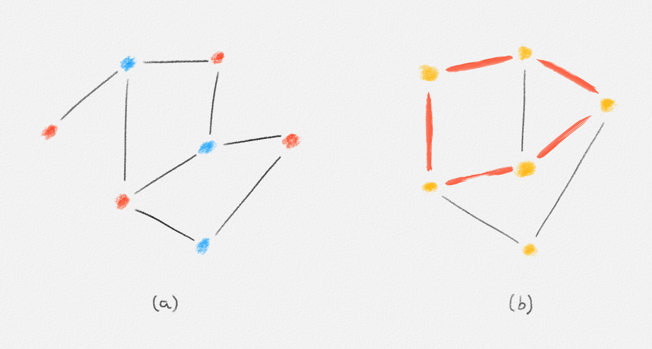
Figure 7.1: The graph in (a) is bipartite because every edge has a red endpoint and a blue endpoint. In other words, the partition of the vertex set into the set \(U\) containing all red vertices and the set \(W\) containing all blue vertices proves that the graph is bipartite. By Exercise 7.2, the graph in (b) is not bipartite because of the odd cycle formed by the red edges.

Back to scheduling jobs on machines. If a job \(j \in J\) can run on a machine \(m \in M\) (some jobs may not be possible to run on a given machine at all, for example, if the job has high memory requirements and the machine has too little memory), then there is an edge \((j, m) \in G\) with weight equal to the cost of running job \(j\) on machine \(m\). If we assume that we want to run every job on a different machine, our goal is to pick a subset of the edges in \(G\) such that no two edges share an endpoint (no two jobs run on the same machine and no job can be split over multiple machines), every vertex in \(J\) is the endpoint of a chosen edge (we run every job), and the total weight of the chosen edges is minimized.

A set \(M\) of edges in a graph such that no two edges in \(M\) share an endpoint is called a matching. For every edge \((x,y) \in M\), we call \(x\) and \(y\) mates. See Figure 7.2.

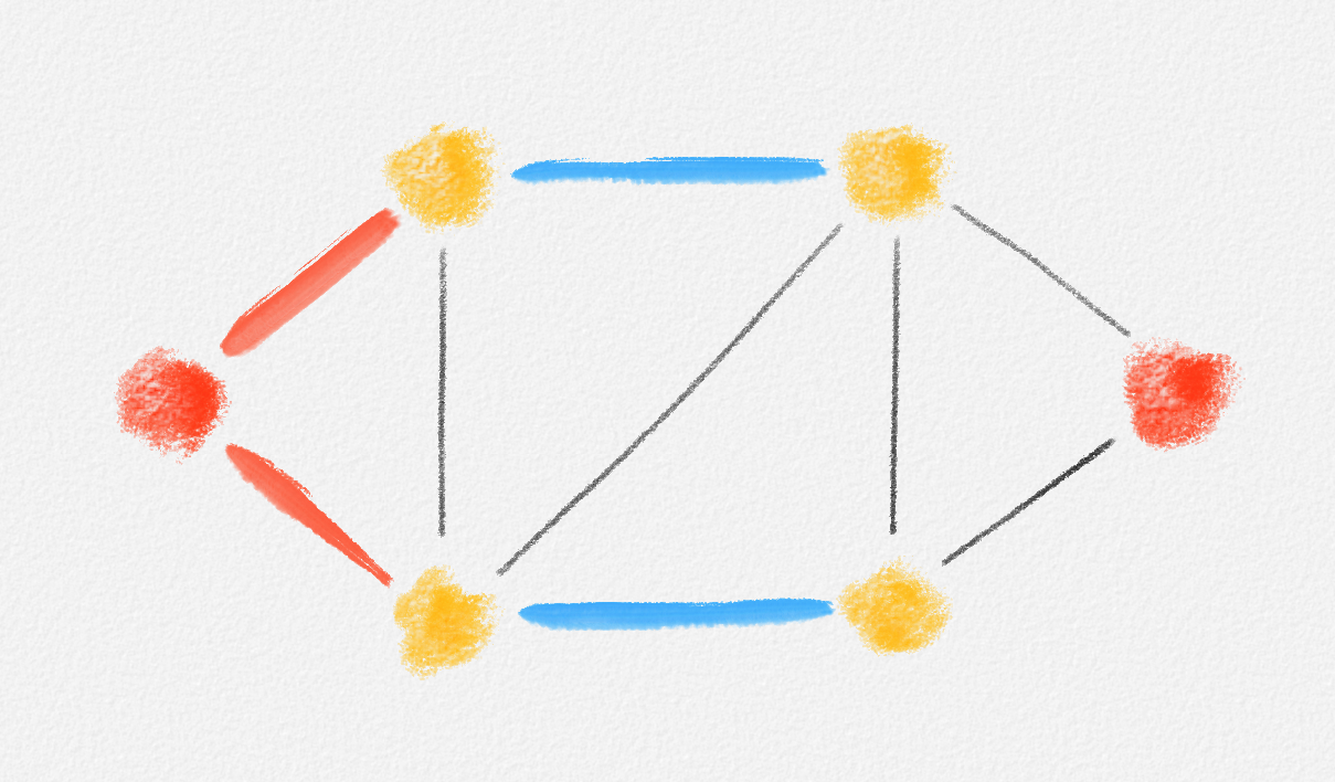
Figure 7.2: The blue edges form a matching, as these edges do not have any endpoints in common. The red edges do not form a matching, as they share an endpoint.

Throughout this chapter, we refer to a vertex \(x\) of a graph \(G\) as matched by a matching \(M\) if \(x\) is an endpoint of an edge in \(M\); otherwise, \(x\) is unmatched by \(M\). If the matching is clear from the context, we will refer to vertices simply as matched or unmatched, without specifying the matching. We also refer to edges as matched or unmatched depending on whether they belong to \(M\).

If every vertex of \(G\) is the endpoint of an edge in \(M\), then \(M\) is called a perfect matching. See Figure 7.3.

Figure 7.3: The blue edges in Figure 7.2 do not form a perfect matching because the two red vertices are unmatched. The red edges in this figure do form a perfect matching because every vertex is an endpoint of a red edge. The blue edges in this figure also form a perfect matching. The blue edges do not form a minimum-weight perfect matching because the red edges have lower total cost. You can check that there is no perfect matching of lower cost than the red edges, so the red edges form a minimum-weight perfect matching.

In the above scenario of scheduling jobs on machines, if the number of jobs equals the number of available machines, then the requirement that every job has an incident edge in the matching implies that every machine also has an incident edge in the matching. Thus, we are looking for a minimum-weight perfect matching:

Given a graph \(G = (V, E)\) and a cost function \(c : E \rightarrow \mathbb{R}\), a minimum-weight perfect matching is a perfect matching \(M\) such that no perfect matching of \(G\) has lower cost. See Figure 7.3.

Such a matching may not exist since there may be pairs of vertices not connected by an edge. Thus, we may also consider the simpler problem of deciding whether a perfect matching exists. This decision problem can be generalized to the maximum-cardinality matching problem, which is to find a matching containing as many edges as possible.

Given a graph \(G\), a maximum-cardinality matching is a matching \(M\) of \(G\) such that no matching of \(G\) contains more edges than \(M\).

Observation 7.1: A matching \(M\) of an \(n\)-vertex graph \(G\) is a perfect matching if and only if it has size \(\frac{n}{2}\).

In the same way we went from the minimum-weight perfect matching problem to the simpler problem of finding a perfect matching, we can generalize the maximum-cardinality matching problem to the maximum-weight matching problem, which asks us to find a matching of maximum weight.

Given a graph \(G = (V, E)\) and a cost function \(c : E \rightarrow \mathbb{R}\), a maximum-weight matching is a matching \(M\) such that no matching of \(G\) has greater cost. The cost of a matching is the total cost of its edges: \(c(M) = \sum_{e \in M} c_e\).

Note that a maximum-weight matching may contain fewer edges than a maximum-cardinality matching for the same graph if the edge costs in the graph vary sufficiently. An example is shown in Figure 7.4.

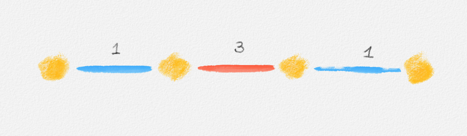
Figure 7.4: The blue edges are a maximum-cardinality matching: The matching is perfect, so there cannot be any bigger matching. It is not a maximum-weight matching because the red edge has a greater cost than the total cost of the two blue edges. The set containing only the red edge is a maximum-weight matching but not a maximum-cardinality matching because the matching consisting of the blue edges contains more edges.

Exercise 7.1: Prove that it is possible to adjust the costs in a weighted graph so that a maximum-weight matching with respect to the adjusted costs is

• A matching of maximum cost (with respect to the original costs) among all maximum-cardinality matchings of the graph or

• A matching of maximum cardinality among all maximum-weight matchings (with respect to the original costs) of the graph.

The final generalization we consider is to drop the requirement that the given graph be bipartite. Many natural applications of matching problems work with bipartite graphs and, as we will see, solving matching problems on bipartite graphs can be significantly easier than on arbitrary graphs. Nevertheless, it is useful to be able to find various kinds of matchings in arbitrary graphs, particularly as a building block for other algorithms.

Since bipartite graphs play a central role throughout most of this chapter, here are two exercises that help you get more comfortable thinking about the structure of bipartite graphs:

Exercise 7.2: Prove that a graph is bipartite if and only if it contains no odd cycle (cycle of odd length).

Exercise 7.3: Show that if a bipartite graph \(G = (V, E)\) is connected, then there exists exactly one partition of \(V\) into two disjoint subsets \(U\) and \(W\) such that every edge has one endpoint in \(U\) and the other in \(W\). Prove that in general, a non-empty bipartite graph with \(k\) connected components has \(2^{k-1}\) such partitions of its vertex set into subsets \(U\) and \(W\).

7.2. Maximal Matching

As a warm-up exercise, this section discusses the maximal matching problem. Given a graph \(G = (V, E)\), the problem is to find a matching \(M \subseteq E\) such that there is no matching \(M'\) that satisfies \(M \subset M' \subseteq E\). As an example, the blue matching \(M\) in Figure 7.2 is maximal because every edge not in \(M\) shares an endpoint with an edge in \(M\) and therefore cannot be added to \(M\) while keeping \(M\) a matching. \(M\) is not a maximum matching because both matchings in Figure 7.3 are bigger.

The algorithm to compute a maximal matching is extremely simple: We start by setting \(M = \emptyset\). Then we inspect every edge \(e \in E\) in turn. When inspecting \(e\), we add \(e\) to \(M\) if and only if \(e\)'s endpoints are unmatched at this time.

This algorithm can clearly be implemented in \(O(n + m)\) time using an adjacency list representation of the graph, which allows us to enumerate the vertices and edges of \(G\) in linear time and find the endpoints of each edge in constant time: First, we mark every vertex as unmatched; this takes \(O(n)\) time. Then we inspect every edge \(e \in E\). For each edge \((x, y)\), we check whether both \(x\) and \(y\) are unmatched. If so, we add \((x,y)\) to \(M\) and mark \(x\) and \(y\) as matched. This takes constant time per edge, \(O(m)\) time in total.

Lemma 7.2: A maximal matching of a graph \(G\) can be computed in \(O(n + m)\) time.

Proof: We already argued that the above algorithm takes \(O(n + m)\) time. To see that its output is a matching, assume the contrary. Then there exist two edges \(e\) and \(f\) in \(M\) that share an endpoint \(x\). If w.l.o.g. \(e\) is added to \(M\) before \(f\), then \(x\) is marked as matched after adding \(e\) to \(M\). Thus, when inspecting \(f\), \(x\) is matched, and we do not add \(f\) to \(M\), a contradiction.

To see that the computed matching \(M\) is maximal, assume that there exists an edge \((x,y) \in E\) such that \(M \cup \{(x,y)\}\) is also a matching. Then both \(x\) and \(y\) are unmatched at the end of the algorithm and thus also when the algorithm inspects the edge \((x,y)\). Therefore, we would have added \((x,y)\) to \(M\), a contradiction. ▨

A related problem is the independent set problem.

An independent set in a graph \(G = (V,E)\) is a subset \(I \subseteq V\) such that no two vertices in \(I\) are adjacent. See Figure 7.5.

Figure 7.5: A maximal but not maximum independent set (blue) and a maximum independent set (red). Both sets are vertex covers. The blue set is a minimum vertex cover, the red one is not.

Again, we can distinguish between a maximal independent set, which has no independent proper superset, and a maximum independent set, which is an independent set of maximum cardinality.

Exercise 7.4: Show that a maximal independent set of an arbitrary graph can be computed in \(O(n + m)\) time. (Hint: The algorithm is very similar to the maximal matching algorithm above.)

The maximum-cardinality variants of matching and independent set, on the other hand, are of very different difficulty. While the focus of this chapter is to demonstrate that a wide range of matching problems can be solved in polynomial time, finding a maximum independent set is NP-hard and in fact W[1]-hard, that is, unlikely to be fixed-parameter tractable. We will discuss fast exponential-time algorithms for finding a maximum independent set in Chapters 16 and 17.

Matchings are closely related to another classical NP-hard problem, the vertex cover problem, which is to find a minimum-size subset \(C\) of \(G\)'s vertices such that every edge of \(G\) has at least one endpoint in \(C\) (see Figure 7.5). Based on this connection, the matching algorithms discussed in this chapter will be used in fixed-parameter algorithms for the vertex cover problem.

7.3. Bipartite Matching via Network Flows

In this section, we discuss that the maximum-cardinality matching problem, the maximum-weight matching problem, and the minimum-weight perfect matching problem in bipartite graphs can be solved using network flow algorithms. The maximum-cardinality matching problem can be expressed as a maximum flow problem. The maximum-weight matching problem and the minimum-weight perfect matching problem can be expressed as minimum-cost flow problems.

7.3.1. Maximum-Cardinality Matching

Let us start with finding a maximum-cardinality matching in a bipartite graph \(G = (U, W, E)\). To find such a matching, we augment \(G\) with two new vertices \(s\) and \(t\). Every vertex in \(U\) becomes an out-neighbour of \(s\), every vertex in \(W\) becomes an in-neighbour of \(t\), and every edge of \(G\) gets directed from its endpoint in \(U\) to its endpoint in \(W\). Finally, we give every edge a capacity of \(1\). Let us call the resulting graph \(\vec{G}\). This construction is illustrated in Figure 7.6.

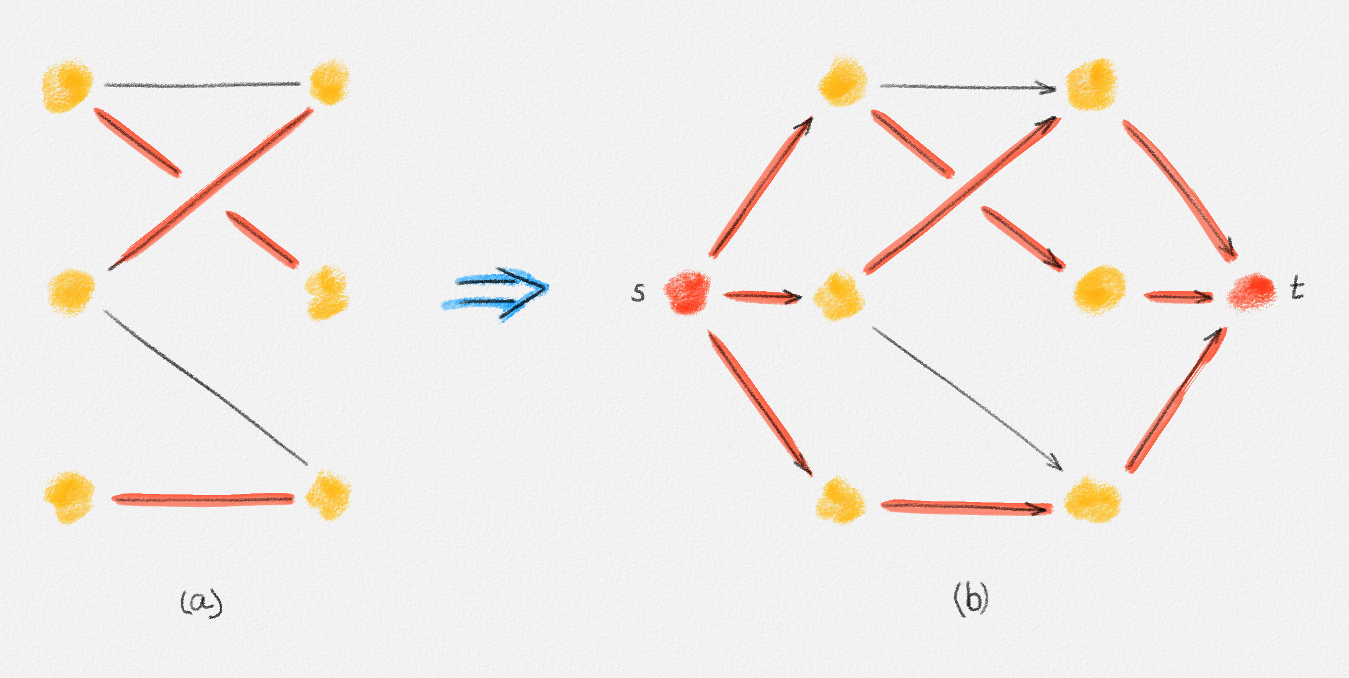
Figure 7.6: (a) A bipartite graph \(G\) and a maximum-cardinality matching shown in red. (b) The graph \(\vec{G}\) constructed from \(G\) by directing all edges from left to right, adding two vertices \(s\) and \(t\), and making all vertices in \(U\) out-neighbours of \(s\) and all vertices in \(W\) in-neighbours of \(t\). All edges have capacity \(1\). The maximum-flow corresponding to the maximum matching in (a) sends one unit of flow along each of the red \(st\)-paths.

Lemma 7.3: \(M\) is a matching in \(G\) if and only if there exists an integral \(st\)-flow \(f\) in \(\vec{G}\) such that \(M = \{e \in G \mid f_e = 1\}\).

Proof: First assume that \(M\) is a matching. Then set \(f_{s,u} = f_{u,w} = f_{w,t} = 1\) for every edge \((u,w) \in M\) and \(f_e = 0\) for any other edge. Clearly, \(f\) is integral and satisfies the capacity constraints of all edges in \(\vec{G}\). For every vertex \(u \in G\), if \(u\) is unmatched, then \(f_{s,u} = 0\) and \(f_{u,w} = 0\) for every edge \((u,w) \in G\). If \(u\) is matched, then \(f_{s,u} = 1\) and \(f_{u,w} = 1\) for exactly one edge \((u,w) \in G\) because \(M\) is a matching. Thus, \(f\) satisfies \(u\)'s flow conservation constraint whether \(u\) is matched or not. A similar argument shows that \(f\) satisfies the flow conservation constraints of all vertices in \(W\). Thus, \(f\) is an \(st\)-flow.

Now assume that \(f\) is an integral \(st\)-flow in \(\vec{G}\). By the flow conservation constraint, we have \(\sum_{w \in W} f_{u,w} = f_{s,u} \le 1\) for every vertex \(u \in U\). Since \(f\) is integral, this shows that there exists at most one edge \((u,w) \in G\) such that \(f_{u,w} = 1\). By an analogous argument, there exists at most one edge \((u,w) \in G\) such that \(f_{u,w} = 1\) for every vertex \(w \in W\). Thus, the set \(M = \{e \in G \mid f_e = 1\}\) is a matching in \(G\). ▨

Corollary 7.4: A maximum-cardinality matching of a bipartite graph \(G\) can be found in \(O\bigl(n^2 \sqrt{m}\bigr)\) time.

Proof: Constructing \(\vec{G}\) from \(G\) takes \(O(n + m)\) time. By Theorem 5.34, we can find a maximum flow \(f\) in \(\vec{G}\) in \(O\bigl(n^2 \sqrt{m}\bigr)\) time. By Observation 5.35, this flow is integral. Thus, by Lemma 7.3, the set \(M = \{e \in G \mid f_e = 1\}\) is a matching in \(G\). Constructing \(M\) from \(f\) takes \(O(n + m)\) time. Overall, computing \(M\) thus takes \(O\bigl(n^2\sqrt{m}\bigr)\) time.

Since \(U \cup \{s\}\) is an \(st\)-cut in \(\vec{G}\) and every edge in \(G\) crosses this cut, we have \(|M| = F_s\), by Lemma 5.3. If \(M\) is not a maximum-cardinality matching, then there exists a matching \(M'\) such that \(|M'| > |M|\). By Lemma 7.3, \(M' = \{e \in G \mid f'_e = 1\}\), for some integral \(st\)-flow \(f'\) in \(\vec{G}\). Again, since \(U \cup \{s\}\) is an \(st\)-cut, we have \(F'_s = |M'| > |M| = F_s\), a contradiction because \(f\) is a maximum flow in \(\vec{G}\). This proves that \(M\) is a maximum-cardinality matching in \(G\). ▨

7.3.2. Maximum-Weight Matching

Finding a maximum-weight matching via network flows is a little harder than finding a maximum-cardinality matching because we cannot easily reduce it to finding a maximum flow; we need to find a minimum-cost flow instead. Once again, we turn the bipartite graph \(G = (U, W, E)\) into a directed network \(\vec{G}\) as in the previous subsection. Again, every edge has capacity \(1\). The cost of every edge incident to \(s\) or \(t\) is \(0\). The cost of every edge \((u, w)\) with \(u \in U\) and \(w \in W\) is the negation of this edge's cost in \(G\). Finally, we add an uncapacitated edge \((s, t)\) of cost zero to \(\vec{G}\). The supply balance of every vertex in \(U \cup W\) is \(0\), \(b_s = |U|\), and \(b_t = -|U|\). This construction is shown in Figure 7.7.

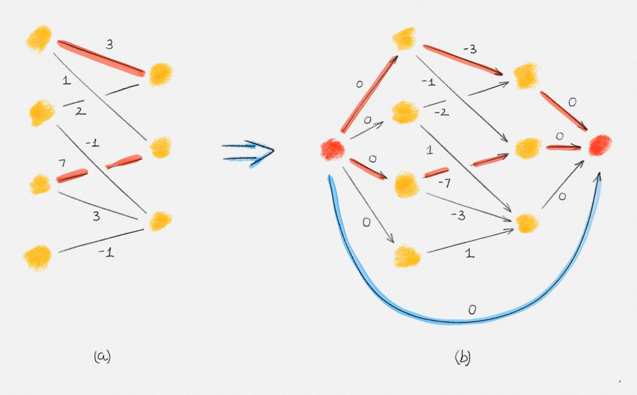
Figure 7.7: (a) A bipartite graph \(G\) and a maximum-weight matching of \(G\) shown in red. The edge labels are edge costs. (b) The graph \(\vec{G}\) obtained from \(G\) by adding two vertices \(s\) and \(t\), directing all edges of \(G\) from left to right, making all vertices in \(U\) out-neighbours of \(s\), making all vertices in \(W\) in-neighbours of \(t\), and adding an edge from \(s\) to \(t\). All edges incident to \(s\) or \(t\) have cost \(0\). The cost of any other edge is the negation of the cost of its corresponding edge in \(G\). All edges except the edge \((s, t)\) have capacity \(1\). The edge \((s, t)\) is uncapacitated. Edge capacities are not shown. Vertex supply balances are not shown. \(s\) has supply balance \(|U| = 4\). \(t\) has supply balance \(-|U| = -4\). All other supply balances are \(0\). The minimum-cost flow corresponding to the maximum-weight matching in (a) is shown in red and blue. One unit of flow is sent along each of the red \(st\)-paths. The remainder of the flow, \(2\) units of flow, is sent from \(s\) to \(t\) along the blue edge, at cost \(0\).

Lemma 7.5: \(M\) is a matching in \(G\) if and only if there exists an integral flow \(f\) in \(\vec{G}\) such that \(M = \{e \in G \mid f_e = 1\}\). The cost of \(M\) is the negation of the cost of \(f\).

Proof: The proof that \(M\) is a matching in \(G\) if and only if there exists an integral flow \(f\) in \(\vec{G}\) such that \(M = \{e \in G \mid f_e = 1\}\) is analogous to the proof of Lemma 7.3. We only need to observe that \(|U|\) is the maximum cardinality of any matching in \(G\) and that any amount of flow not sent from \(s\) to \(t\) via a path that includes a vertex in \(U\) and a vertex in \(W\) can be sent via the uncapacitated edge \((s,t)\).

To see that the cost of \(M\) is the negation of the cost of \(f\), observe that every edge in \(\vec{G}\) has cost \(0\), except edges \((u,w)\) with \(u \in U\) and \(w \in W\). For any such edge \(e\), its cost in \(\vec{G}\) is the negation of its cost in \(G\). Since \(e \in M\) if and only if \(f_e = 1\), this shows that \(M\)'s cost is the negation of the cost of \(f\). ▨

Corollary 7.6: A maximum-weight matching of a bipartite graph \(G\) can be found in \(O((n \lg n + m)m \lg n)\) time.

Proof: Constructing \(\vec{G}\) from \(G\) takes \(O(n + m)\) time. By Theorem 6.75, we can find a minimum-cost flow \(f\) in \(\vec{G}\) in \(O((n \lg n + m)m \lg n)\) time. As observed in Section 5.3, this flow is integral. Thus, by Lemma 7.5, the set \(M = \{e \in G \mid f_e = 1\}\) is a matching in \(G\). Constructing \(M\) from \(f\) takes \(O(n + m)\) time. Therefore, the whole procedure for computing \(M\) takes \(O((n \lg n + m)m \lg n)\) time.

Next assume that \(M\) is not a maximum-weight matching. Then there exists a matching \(M'\) of greater cost. By Lemma 7.5, \(M' = \{e \in G \mid f'_e = 1\}\) for some integral flow \(f'\) in \(\vec{G}\). Moreover, the cost of \(f'\) is the negation of the cost of \(M'\). Since the same is true for \(f\) and \(M\), this implies that \(f'\) has a lower cost than \(f\), a contradiction because \(f\) is a minimum-cost flow. This proves that \(M\) is a maximum-weight matching. ▨

7.3.3. Minimum-Weight Perfect Matching

The reduction of the minimum-weight perfect matching problem to a minimum-cost flow problem is similar to the reduction of the maximum-weight matching problem to a minimum-cost flow problem:

Lemma 7.7: It takes \(O\bigl(n^2 \sqrt{m}\bigr)\) time to decide whether a bipartite graph has a perfect matching. If such a matching exists, a minimum-weight perfect matching can be found in \(O\bigl(n^2 \lg n + nm\bigr)\) time.

Proof: If \(|U| \ne |W|\), the algorithm can terminate immediately because no perfect matching exists. If \(|U| = |W| = n\), a perfect matching is any matching of size \(n\), and there exists no larger matching. Thus, we find a maximum-cardinality matching in \(O(n^2\sqrt{m})\) time, using Corollary 7.4, and then compare the size of the computed matching to \(n\). If the matching has size \(n\), it is a perfect matching. Otherwise, there is no perfect matching.

If there exists a perfect matching, we are now interested in finding a matching of size \(n\) whose cost is minimized. This can be done in almost the same way as in Corollary 7.6. We construct the network \(\vec{G}\) as in the maximum-weight matching problem but (a) do not add the edge \((s,t)\) and (b) choose the cost of every edge \((u,w)\) with \(u \in U\) and \(w \in W\) to be equal to its cost in \(G\). Then it is easy to verify that every flow in \(\vec{G}\) sends one unit of flow along exactly one of the out-edges of every vertex in \(U\) and along exactly one in-edge of every vertex in \(W\). Thus, it corresponds to a perfect matching. Since we minimize the cost of the flow, the computed matching has minimum cost among all perfect matchings.

In fact, the addition of the two vertices \(s\) and \(t\) when computing a maximum-weight matching was necessary only because we did not know the cardinality of a maximum-weight matching. Thus, we (a) did not know which vertices in \(U\) have any incident edges in the computed matching and (b) needed a way to divert flow from \(s\) to \(t\) via the edge \((s,t)\) if this gives us the cheapest flow. In the minimum-weight perfect matching problem, we send exactly one unit of flow from every vertex \(u \in U\) to some vertex \(w \in W\) and every vertex \(w \in W\) receives exactly one unit of flow from some vertex \(u \in U\). Thus, we can simplify \(\vec{G}\) by removing \(s\), \(t\), and their incident edges and instead setting \(b_u = 1\) for every vertex \(u \in U\) and \(b_w = -1\) for every vertex \(w \in W\). This is illustrated in Figure 7.8 and has the benefit that the maximum capacity and the maximum absolute node supply are now \(1\), so the successive shortest paths algorithm is faster than the enhanced capacity scaling algorithm; its running time is \(O\bigl(n^2 \lg n + nm\bigl)\) if \(U = 1\) while the enhanced capacity scaling algorithm takes \(O((n \lg n + m) m \lg n)\) time. ▨

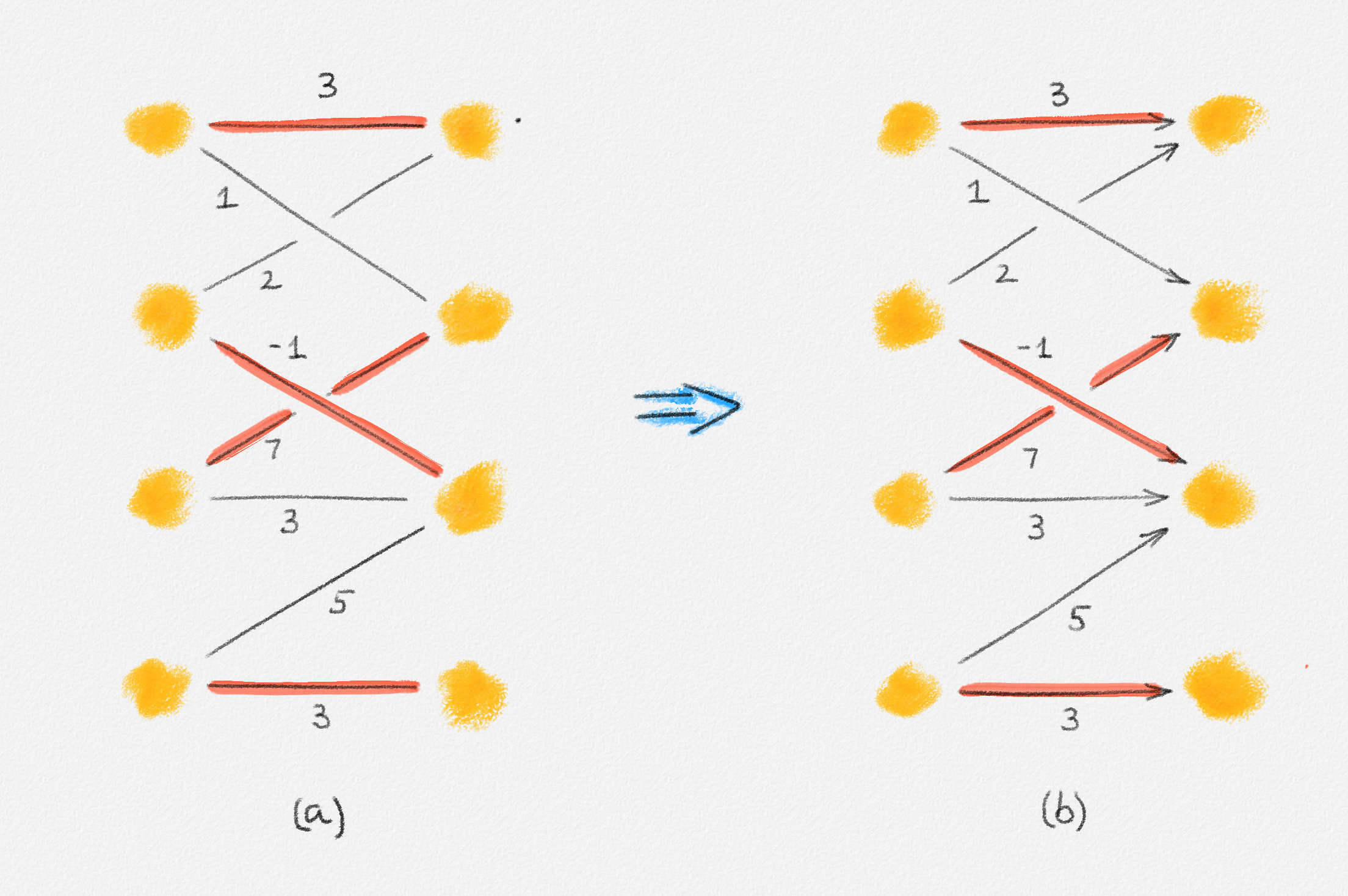
Figure 7.8: (a) A bipartite graph \(G\) and a minimum-weight perfect matching of \(G\) shown in red. The edge labels are edge costs. (b) The graph \(\vec{G}\) obtained from \(G\) by directing all edges of \(G\) from left to right. Edge costs are not negated in this construction, and no verices or edges are added. All edges have capacity \(1\) (not shown). Every vertex in \(U\) has supply balance \(1\). Every vertex in \(W\) has supply balance \(-1\). Vertex supply balances are not shown. The minimum-cost flow corresponding to the minimum-weight perfect matching in (a) sends one unit of flow along each of the red edges.

We will soon discuss a reduction of the maximum-weight matching problem in a graph \(G\) with \(n\) vertices and \(m\) edges to the minimum-weight perfect matching problem in a graph \(G'\) with \(2n\) vertices and \(2m + n\) edges. If \(G\) is bipartite, then so is \(G'\). Thus, we can in fact find a maximum-weight matching in \(O\bigl(n^2 \lg n + nm\bigr)\) time using the successive shortest paths algorithm, an improvement over the bound proven in Corollary 7.6.

7.4. Bipartite Maximum-Cardinality Matching

We have shown in Section 7.3 that a maximum-cardinality, maximum-weight or minimum-weight perfect matching in a bipartite graph can be found in polynomial time by transforming the problem into a maximum flow or minimum-cost flow problem in some network \(\vec{G}\). Next we show that all these types of matchings can be found more efficiently, without the detour via network flows. We start by discussing the maximum-cardinality matching problem, still in bipartite graphs.

• Section 7.4.1 introduces the key concept we use to find matchings of various kinds: augmenting paths. All matching algorithms start with some matching, often the trivial matching \(M = \emptyset\), and then look for augmenting paths to make the matching bigger. We prove that a matching is a maximum-cardinality matching if and only if there does not exist an augmenting path with respect to this matching.

  Note the similarity to augmenting path maximum-flow algorithms. Those algorithms start with the trivial flow \(f = 0\) and then look for augmenting paths along which to send more flow from \(s\) to \(t\). Just as we claim here that a matching is a maximum-cardinality matching if and only if it has no augmenting path, we proved that a flow is a maximum \(st\)-flow if and only if there exists no augmenting path for this flow. The only difference is that we now talk about a different kind of augmenting path, because we want to construct matchings, not flows.

• Section 7.4.2 introduces alternating forests as a tool for finding augmenting paths. We prove that such a forest can be found in \(O(n + m)\) time using an adaptation of breadth-first search (BFS), called alternating BFS and that such a forest can be used to decide whether a bipartite graph has an augmenting path for a given matching and, if so, find one. Note that this latter part relies crucially on the graph being bipartite: If the graph is not bipartite, then deciding whether there exists an augmenting path and finding such a path are much harder, as we will see in Section 7.7.

• The algorithms for finding an alternating forest and for using it to find an augmenting path in a bipartite graph, discussed in Section 7.4.2, immediately lead to a simple \(O(nm)\)-time algorithm to find a maximum-cardinality matching in a bipartite graph. We discuss this algorithm in Section 7.4.3.

• Most algorithms we discuss in this chapter find one augmenting path at a time. In Section 7.4.4, we discuss the Hopcroft-Karp algorithm, which applies a strategy reminiscent of Dinitz's maximum flow algorithm to find many augmenting paths simultaneously—the parallel to maximum flow algorithms continues. This allows the Hopcroft-Karp algorithm to find a maximum-cardinality matching in a bipartite graph in \(O\bigl(n + m\sqrt{n}\bigr)\) time.

7.4.1. Augmenting Paths

In this section, we introduce augmenting paths, the key concept needed in all matching algorithms for both bipartite and arbitrary graphs.

Given a matching \(M\) in a graph \(G\), bipartite or not, an alternating path is a path in \(G\) whose edges alternate between being in \(M\) and not being in \(M\). We call an alternating path even or odd if it is a path of even or odd length.

An alternating cycle is a cycle of even length whose edges alternate between being in \(M\) and not being in \(M\).

An augmenting path is an alternating path both of whose endpoints are unmatched.

In particular, an augmenting path must have odd length and must start and end with an unmatched edge. These definitions are illustrated in Figure 7.9.

Figure 7.9: A graph \(G\) and a matching \(M\) (the red edges). The red, blue, and yellow shaded paths are alternating for \(M\). The red path is augmenting because its endpoints are both unmatched. The green path is not alternating because it contains two consecutive unmatched edges. For the red path \(R\) and the blue path \(B\), \(M \oplus R\) and \(M \oplus B\) are matchings. For the yellow path \(Y\), \(M \oplus Y\) is not a matching because its left endpoint is matched by an edge not in \(Y\).

For two edge sets \(E_1\) and \(E_2\), let \(E_1 \oplus E_2 = (E_1 \setminus E_2) \cup (E_2 \setminus E_1)\). The following lemma and its corollary give a useful characterization of maximum-cardinality matchings. See Figure 7.10 for an illustration.

Lemma 7.8: For two matchings \(M_1\) and \(M_2\), \(M_1 \oplus M_2\) is a collection of paths \(P_1, \ldots, P_k\) and cycles \(C_1, \ldots, C_\ell\). If \(a_1\) is the number of augmenting paths for \(M_1\) among \(P_1, \ldots, P_k\) and \(a_2\) is the number of augmenting paths for \(M_2\) among \(P_1, \ldots, P_k\), then \(|M_1| = |M_2| - a_1 + a_2\).

Figure 7.10: The symmetric difference \(M_1 \oplus M_2\) (shaded yellow) of two matchings \(M_1\) (red edges) and \(M_2\) (blue edges) is composed of a collection of alternating paths and cycles. In this example, one of the paths is an augmenting path for \(M_1\) and there are no augmenting paths for \(M_2\). Thus, \(|M_2| = |M_1| + 1\).

Proof: Every vertex has at most one incident edge in \(M_1\) and at most one incident edge in \(M_2\). Thus, it has at most two incident edges in \(M_1 \oplus M_2\). Since this is true for every vertex, \(M_1 \oplus M_2\) is a collection of paths and cycles.

We have \(|M_1| = |M_1 \cap M_2| + |M_1 \setminus M_2|\) and \(|M_2| = |M_1 \cap M_2| + |M_2 \setminus M_1|\). Thus,

\[\begin{aligned} |M_1| - |M_2| &= |M_1 \setminus M_2| - |M_2 \setminus M_1|\\ &= |M_1 \cap (M_1 \oplus M_2)| - |M_2 \cap (M_1 \oplus M_2)|\\ &= \sum_{i=1}^k\ \bigl(|M_1 \cap P_i| - |M_2 \cap P_i|\bigr) + \sum_{i=1}^\ell\ \bigl(|M_1 \cap C_i| - |M_2 \cap C_i|\bigr). \end{aligned}\]

Since \(M_1\) and \(M_2\) are matchings, the edges in every path \(P_i\) and every cycle \(C_i\) alternate between being in \(M_1\) and \(M_2\). Thus, every cycle \(C_i\) has even length and contains the same number of edges from \(M_1\) and \(M_2\), that is, \(|M_1 \cap C_i| - |M_2 \cap C_i| = 0\) for all \(1 \le i \le \ell\). Similarly, every even-length path \(P_i\) contains the same number of edges from \(M_1\) and \(M_2\), that is, \(|M_1 \cap P_i| - |M_2 \cap P_i| = 0\) for any such path.

Every odd-length path either contains one more edge from \(M_1\) than from \(M_2\) or one more edge from \(M_2\) than from \(M_1\). Let \(\mathcal{P}_1\) be the set of paths that contain one more edge from \(M_2\) than from \(M_1\), and let \(\mathcal{P}_2\) be the set of paths that contain one more edge from \(M_1\) than from \(M_2\). Then

\[|M_1| - |M_2| = |\mathcal{P}_2| - |\mathcal{P}_1|.\]

Next we prove that a path among \(P_1, \ldots, P_k\) belongs to \(\mathcal{P}_1\) if and only if it is an augmenting path for \(M_1\). By symmetry, a path among \(P_1, \ldots, P_k\) belongs to \(\mathcal{P}_2\) if and only if it is an augmenting path for \(M_2\). Thus, \(|\mathcal{P}_1| = a_1\), \(|\mathcal{P}_2| = a_2\), and \(|M_1| = |M_2| - a_1 + a_2\), as claimed.

So consider a path \(P_i\) in \(\mathcal{P}_1\). Since \(P_i\) is an alternating path with respect to \(M_1\), to prove that \(P_i\) is an augmenting path for \(M_1\), we need to prove that its endpoints \(x\) and \(y\) are unmatched by \(M_1\). Consider \(x\). The proof that \(y\) is unmatched is analogous. Since the edges in \(P_i\) alternate between \(M_1\) and \(M_2\), and \(P_i\) contains one more edge from \(M_2\) than from \(M_1\), the edge \(e\) in \(P_i\) incident to \(x\) is in \(M_2\) and, since it is in \(M_1 \oplus M_2\), not in \(M_1\). Thus, if \(x\) were matched by \(M_1\), then the edge \(f\) in \(M_1\) incident to \(x\) would have to be a different edge, \(f \ne e\). Since \(e \in M_2\) and \(M_2\) is a matching, we have \(f \notin M_2\), so \(f \in M_1 \oplus M_2\). This shows that \(x\) would have two incident edges in \(M_1 \oplus M_2\), but being the endpoint of \(P_i\), it has degree one in \(M_1 \oplus M_2\). This is a contradiction, so \(x\) must be unmatched.

Now consider a path \(P_i\) that is an augmenting path for \(M_1\). By the definition of an augmenting path, \(P_i\) is an alternating path with respect to \(M_1\) whose endpoints are unmatched by \(M_1\). Thus, the first and last edges of \(P_i\) do not belong to \(M_1\). This implies that \(P_i\) has one more edge from \(M_2\) than from \(M_1\), that is, \(P_i \in \mathcal{P}_1\). ▨

The following corollary provides the characterization of a maximum-cardinality matching that all matching algorithms in this chapter are based on:

Corollary 7.9: A matching \(M\) is a maximum-cardinality matching if and only if there is no augmenting path in \(G\) with respect to \(M\). For an augmenting path \(P\), \(M' = M \oplus P\) is a matching of cardinality \(|M'| = |M| + 1\).

Proof: First assume that there exists an augmenting path \(P\) with respect to \(M\) and let \(M' = M \oplus P\). Note that \(M'\) is a matching: If it is not, then there exists a vertex \(x\) with two incident edges \(e, f \in M'\). At most one of these edges is in \(M\) because \(M\) is a matching. The other, say \(e\), is therefore in \(P \setminus M\). Since \(P\) is an augmenting path, all edges incident to the endpoints of \(e\), other than \(e\) itself, are in \(E \setminus (M \cup P)\) or in \(M \cap P\). None of these edges is in \(M' = (M \setminus P) \cup (P \setminus M)\), so \(x\) cannot have a second edge in \(M'\), \(f\), incident to it.

Next observe that \(M \oplus M' = P\). Since \(P\) is an augmenting path for \(M\), Lemma 7.8 shows that \(|M'| = |M| + 1\), that is, \(M\) is not a maximum-cardinality matching and the second part of the corollary holds.

Conversely, if \(M\) is not a maximum-cardinality matching, then let \(M'\) be a maximum-cardinality matching. Since \(|M'| > |M|\), one of the paths in \(M \oplus M'\) must be an augmenting path for \(M\), by Lemma 7.8. Thus, the first part of the corollary holds. ▨

7.4.2. Alternating Forests and Alternating BFS

A key tool in many matching algorithms is the alternating forest:

Given a graph \(G\) and a matching \(M\) in \(G\), an alternating forest is a rooted forest \(F \subseteq G\) whose roots are unmatched and such that every path in \(F\) from a root to one of its descendants is an alternating path. See Figure 7.11. Note that there is no requirement that \(F\) contains all vertices of \(G\).

For a vertex \(x \in F\), we denote the tree in \(F\) that contains \(x\) as \(T_x\), the root of \(T_x\) as \(r_x\), and the path from \(r_x\) to \(x\) in \(T_x\) as \(P_x\).

For every vertex \(x \in F\), we refer to the depth of \(x\) in \(F\), that is, to the length of \(P_x\) as \(x\)'s level \(\ell^F_x\). We call a vertex \(x \in F\) even or odd depending on whether its level is even or odd.

Figure 7.11: A bipartite graph \(G = (U, W, E)\). Vertices in \(U\) are red. Vertices in \(W\) are blue. The red edges form a matching of \(G\). The yellow shaded subgraph is an alternating forest of \(G\) with all unmatched vertices in \(U\) as the roots. For clarity, this forest is drawn separately below. This separate drawing highlights the level of every vertex and the fact that all top-down paths in the forest are alternating paths. Note that all vertices in \(U\) are on even levels and all vertices in \(W\) are on odd levels.

Given a bipartite graph \(G = (U, W, E)\) and set of unmatched vertices \(R \subseteq U\), we call an alternating forest \(F\) maximum for \(R\) if \(R\) is the set of roots of \(F\) and a vertex \(x\) belongs to \(F\) if and only if there exists an alternating path form a vertex in \(R\) to \(x\).

The algorithm to compute a maximum alternating forest with a given set of roots \(R\) is called alternating BFS because it operates much like breadth-first search (BFS) but alternatingly follows matched and unmatched edges:

We start by marking every vertex in \(G\) as unexplored. Then we mark the vertices in \(R\) as explored, make them the roots of \(F\), and insert them into a queue \(Q\) of vertices whose out-edges are to be explored. Note that this ensures that all vertices in \(Q\) are even and in \(U\). We maintain this invariant throughout the algorithm.

Now, as long as \(Q\) is not empty, we remove the next vertex \(u\) from the head of \(Q\) and inspect all its out-edges. For every edge \((u,w)\) such that \(w\) is unexplored, we mark \(w\) as explored and make \(w\) a child of \(u\) in \(F\). If \(w\) is matched by an edge \((u',w)\), then we also mark \(w\)'s mate \(u'\) as explored, make it \(w\)'s child in \(F\), and add \(u'\) to the end \(Q\). This ensures that \(u'\) is even. Since \(u \in U\) and \(G\) is bipartite, we have \(w \in W\) and \(u' \in U\). So the invariant that \(Q\) contains only even vertices in \(U\) is maintained. Note that we do not need to check whether \(u'\) is explored: Since \(w\) was unexplored and we always add the two endpoints of a matched edge to \(F\) together, \(u'\) is explored if and only if \(w\) is explored.

The final forest \(F\) is the one we obtain once \(Q = \emptyset\).

By the next exercise and lemma, this forest \(F\) is indeed a maximum alternating forest with the vertices in \(R\) as its roots, and this procedure to compute \(F\) takes \(O(n + m)\) time.

Exercise 7.5: Prove that alternating BFS takes \(O(n + m)\) time.

Lemma 7.10: Given a bipartite graph \(G = (U, V, E)\) and a set \(R \subseteq U\) of unmatched vertices, alternating BFS computes a maximum alternating forest \(F\) with the vertices in \(R\) as its roots.

Proof: The forest \(F\) computed by alternating BFS is clearly alternating: Every vertex \(u \in Q\) is even and explored. Thus, if it has a mate, this mate is also explored. Therefore, the child edges of \(u\) added to \(F\) are unmatched. We add a child \(u' \in U\) to an odd vertex \(w\) only if \(u'\) is \(w\)'s mate. Thus, the child edges of odd vertices are matched. Since the child edges of all even vertices are unmatched and the child edges of all odd vertices are matched, \(F\) is an alternating forest.

It remains to prove that \(F\) is maximum for \(R\), that is, that a vertex \(x\) belongs to \(F\) if and only if it can be reached from a vertex in \(R\) via an alternating path.

The "only if" direction is easy because, for every vertex \(x \in F\), the path \(P_x\) is an alternating path from \(r_x \in R\) to \(x\).

For the "if" direction, consider all vertices \(x\) with an alternating path from a vertex in \(R\) to \(x\). For each such vertex \(x\), let \(A_x\) be a shortest alternating path with \(x\) as one of its endpoints and with its other endpoint, \(u_x\), in \(R\). We use induction on \(|A_x|\) to prove that \(x \in F\).

If \(|A_x| = 0\), then \(x = u_x\) and \(x \in R\). Since every vertex in \(R\) is the root of a tree in \(F\), this implies that \(x \in F\).

If \(|A_x| > 0\), then let \(y\) be \(x\)'s predecessor in \(A_x\). The subpath of \(A_x\) from \(u_x\) to \(y\) is an alternating path from \(u_x\) to \(y\) of length less than \(|A_x|\). Since \(A_y\) is a shortest alternating path with \(y\) as one of its endpoints and with the other endpoint in \(R\), this implies that \(|A_y| < |A_x|\). Thus, by the induction hypothesis, \(y \in F\).

If \(x \in U\), then \(A_x\) has even length because \(G\) is bipartite and both endpoints of \(A_x\) are in \(U\). Since \(u_x\) is unmatched, this implies that the edge \((y,x)\) is matched. Since mates are added to \(F\) together and \(y \in F\), this implies that \(x \in F\).

If \(x \in W\), then \(A_x\) has odd length because \(G\) is bipartite and \(A_x\) has one endpoint in \(U\) and the other in \(W\). Since \(u_x\) is unmatched, this implies that the first and last edges of \(A_x\) are both unmatched. Specifically, the edge \((y,x)\) is unmatched. Since \(x \in W\), we have \(y \in U\) because \(G\) is bipartite. Thus, the path \(P_y\) from \(r_y\) to \(y\) in \(F\) has even length. Therefore, \(y\) is even and alternating BFS explores all unmatched edges incident to \(y\). When exploring the edge \((y,x)\), \(x\) becomes \(y\)'s child in \(F\) unless \(x\) is already in \(F\). In either case, \(x \in F\). ▨

Lemma 7.11: Given a bipartite graph \(G\) and a matching \(M\) of \(G\), it takes \(O(n + m)\) time to decide whether there exists an augmenting path \(P\) for \(M\) and, if so, find such a path.

Proof: We use alternating BFS to construct a maximum alternating forest \(F\) whose roots are all the unmatched vertices in \(U\). If \(F\) contains an unmatched vertex \(w \in W\), then the path \(P_w\) from \(r_w\) to \(w\) in \(F\) is an augmenting path because it is an alternating path and both its endpoints are unmatched. Conversely, if there exists an augmenting path \(P\) for \(M\), then it has odd length and therefore must have one endpoint, \(u\), in \(U\) and the other, \(w\), \(W\). Since \(u\) is unmatched, this shows that there exists an alternating path from an unmatched vertex in \(U\) to \(w\). Since \(F\) is a maximum alternating forest, \(w\) is therefore in \(F\).

The algorithm takes \(O(n + m)\) time to construct \(F\), by Exercise 7.5. Given \(F\), it takes \(O(n)\) time to inspect all vertices in \(F\) to check whether one of them is in \(W\) and is unmatched. If we find such a vertex \(w\), we follow parent pointers in \(F\) to construct the augmenting path \(P_w\). Thus, the entire algorithm takes \(O(n + m)\) time. ▨

7.4.3. A Simple \(\boldsymbol{O(nm)}\)-Time Algorithm

The maximum-cardinality matching algorithm discussed in this section is similar in spirit to augmenting path maximum-flow algorithms. We start with the trivial matching \(M = \emptyset\) and then improve the matching by repeatedly finding an augmenting path \(P\) and replacing \(M\) with \(M \oplus P\).¹ Once no augmenting path exists, the current matching \(M\) is a maximum-cardinality matching, by Corollary 7.9, so we return this matching \(M\).

By Lemma 7.11, we can decide whether there exists an augmenting path for the current matching \(M\) and, if so, find such a path \(P\) in \(O(n + m)\) time. Since \(|M \oplus P| > |M|\) for every matching \(M\) and every augmenting path \(P\) for \(M\), and since a matching cannot have more than \(\frac{n}{2}\) edges, the algorithm has at most \(\frac{n}{2}\) iterations. Thus, the running time of the algorithm is \(O((n + m)m)\).

This bound can be improved to \(O(nm)\) using the following simple trick: Observe that an isolated vertex cannot be the endpoint of an edge in the computed matching (because it has no incident edges at all). Thus, we can remove these vertices from \(G\) before running the maximum matching algorithm. This takes \(O(n)\) time. After removing isolated vertices, \(G\) has \(n' \le 2m\) vertices, so each iteration of the maximum matching algorithm now takes \(O(n' + m) = O(m)\) time. The cost of all at most \(\frac{n}{2}\) iterations is thus \(O(nm)\). Adding the \(O(n)\) cost of removing isolated vertices, the cost of the whole algorithm is \(O(n + nm) = O(nm)\). This proves the following lemma:

Lemma 7.12: A maximum-cardinality matching in a bipartite graph can be found in \(O(nm)\) time.

7.4.4. The Hopcroft-Karp Algorithm*

The algorithm for the bipartite maximum-cardinality matching problem discussed in this section improves on the simple algorithm from Section 7.4.3 and achieves a running time of \(O\bigl(n + m\sqrt{n}\bigr)\). This algorithm is due to Hopcroft and Karp. The strategy it uses to improve on the running time of the simple \(O(nm)\)-time algorithm has many parallels to Dinitz's maximum flow algorithm: Instead of finding one augmenting path at a time, we find many such paths in each iteration. To find these paths, we construct a level graph and then use DFS in this graph to find a set of augmenting paths equivalent to a blocking flow. This ensures that the length of a shortest augmenting path increases from one iteration to the next and is the key to proving that the algortihm terminates after \(O\bigl(\sqrt{n}\bigr)\) iterations.

Let us call an augmenting path \(P\) a shortest augmenting path if there is no shorter augmenting path than \(P\).¹

We call a set \(A = \{P_1, \ldots, P_t\}\) of shortest augmenting paths inclusion-maximal if the paths in \(A\) are vertex-disjoint and every shortest augmenting path not in \(A\) shares at least one vertex with some path in \(A\). In this case, \(M \oplus (P_1 \cup \cdots \cup P_t)\) is a matching of size \(|M| + t\).

The Hopcroft-Karp algorithm starts with some matching \(M\) that can be found in \(O(n + m)\) time. The trivial matching \(M = \emptyset\) or a maximal matching fits the bill. Each iteration of the algorithm finds an inclusion-maximal set of shortest augmenting paths \({P_1, \ldots, P_t}\) and replaces \(M\) with \(M \oplus (P_1 \cup \cdots \cup P_t)\). The algorithm ends once there is no augmenting path, that is, once the set of paths found in the current iteration is empty. By Corollary 7.9, \(M\) is a maximum-cardinality matching at this point.

Theorem 7.13: The Hopcroft-Karp algorithm computes a maximum-cardinality matching in a bipartite graph in \(O\bigl(n + m\sqrt{n}\bigr)\) time.

Proof: We just argued that the algorithm computes a maximum-cardinality matching. We prove in Section 7.4.4.1 that an inclusion-maximal set of shortest augmenting paths can be found in \(O(n + m)\) time. If \(G\) has no isolated vertices, then \(n \le 2m\), so finding an inclusion-maximal set of shortest augmenting paths takes \(O(m)\) time. To ensure that \(G\) has no isolated vertices, we remove these vertices from \(G\), which takes \(O(n)\) time. As we show next, the Hopcroft-Karp algorithm runs for \(O\bigl(\sqrt{n}\bigr)\) iterations. Thus, its total running time is \(O\bigl(n + m\sqrt{n}\bigr)\).

By Lemma 7.14 below, after the first \(\sqrt{n}\) iterations, every augmenting path for the current matching \(M\) has length at least \(\sqrt{n}\). Let \(M'\) be a maximum-cardinality matching and let \(S = M \oplus M'\). By Lemma 7.8, \(S\) contains at least \(|M'| - |M|\) vertex-disjoint augmenting paths with respect to \(M\). Since each such path has length at least \(\sqrt{n}\), there are at most \(\sqrt{n}\) such paths. Thus, \(|M'| - |M| \le \sqrt{n}\).

Since each iteration of the Hopcroft-Karp algorithm increases the size of the current matching by at least one, this shows that it takes at most \(\sqrt{n}\) additional iterations to obtain a maximum-cardinality matching. The total number of iterations is thus at most \(2\sqrt{n}\). ▨

Lemma 7.14: Every iteration of the Hopcroft-Karp algorithm increases the length of the shortest augmenting path with respect to the current matching \(M\).

Proof: Let \(M\) be the matching at the beginning of the current iteration, let \(M'\) be the matching at the end of the current iteration, let \(A = \{P_1, \ldots, P_t\}\) be the inclusion-maximal set of shortest augmenting paths we use to construct \(M'\) from \(M\), and let \(k\) be the length of the paths in \(A\).

Consider any augmenting path \(P = \langle v_0, \ldots, v_{k'} \rangle\) with respect to \(M'\). We need to show that \(k' > k\).

If \(P\) is vertex-disjoint from all paths in \(A\), then \(P\) is also an augmenting path for \(M\) and \(A \cup {P}\) is a collection of vertex-disjoint augmenting paths for \(M\). Since \(A\) is an inclusion-maximal set of shortest augmenting paths for \(M\), \(P\) is not a shortest augmenting path for \(M\), that is, \(k' > k\).

So assume that \(P\) shares a vertex \(v\) with at least one path \(P_i\) in \(A\). Let \(S = (P_1 \cup \cdots \cup P_t) \oplus P\). Since \(M' = M \oplus (P_1 \cup \cdots \cup P_t)\), we have \(P_1 \cup \cdots \cup P_t = M \oplus M'\), that is, \(S = (M \oplus M') \oplus P = M \oplus (M' \oplus P)\). \(M' \oplus P\) is a matching of size \(|M'| + 1 = |M| + t + 1\) because \(P\) is an augmenting path for \(M'\). Thus, by Lemma 7.8, \(S\) is a collection of paths and cycles that includes at least \(|M' \oplus P| - |M| = t + 1\) augmenting paths for \(M\). Since any augmenting path for \(M\) has length at least \(k\), the set \(S\) thus contains at least \(k(t+1)\) edges. Since every vertex in \(P_i\) has an incident edge in \(M'\) and the endpoints of \(P\) are unmatched by \(M'\), \(v\) must be an internal vertex of \(P\). Its incident edge in \(M'\) belongs to both \(P_i\) and \(P\) because \(v\) has an incident edge in \(M'\) that belongs to \(P\) and an incident in \(M'\) that belongs to \(P_i\) but \(M'\) is a matching and thus contains at most one edge incident to \(v\). Thus, \(P\) and \(P_i\) share at least one edge. This implies that \(|S| \le |P_1 \cup \cdots \cup P_t \cup P| \le kt + k' - 1\). Since \(|S| \ge k(t+1)\), this gives \(kt + k' - 1 \ge k(t+1)\), that is, \(k' \ge k + 1\). ▨

7.4.4.1. The Level Graph

This section introduces the level graph \(L^M\) for a matching \(M\) of a bipartite graph and shows how to compute \(L^M\) and how use it to find an inclusion-maximal set of shortest augmenting paths, all in \(O(n + m)\) time.

Given a bipartite graph \(G = (U, W, E)\), a subset of unmatched vertices \(R \subseteq U\), and some vertex \(x \in G\), a shortest alternating path from \(\boldsymbol{R}\) to \(\boldsymbol{x}\) is a shortest alternating path \(P\) with the property that one of its endpoints is \(x\) and the other endpoint is in \(R\).

Exercise 7.6: Let \(G = (U, W, E)\) be a bipartite graph, let \(R \subseteq U\) be a subset of unmatched vertices in \(U\), and let \(F\) be a maximum alternating forest of \(G\) with \(R\) as its set of roots computed using alternating BFS. Prove that for every vertex \(x \in F\), the path \(P_x\) from \(r_x \in R\) to \(x\) is a shortest alternating path from \(R\) to \(x\).

Exercise 7.7: Let \(G = (U, W, E)\) be a bipartite graph, let \(R \subseteq U\) be a subset of unmatched vertices in \(U\), and let \(P\) be a shortest alternating path from \(R\) to some vertex \(x\). Let \(r \in R\) be the other endpoint of \(P\), and let \(y\) be any vertex in \(P\). Prove that the subpath of \(P\) from \(r\) to \(y\) is a shortest alternating path from \(R\) to \(y\).

Given a bipartite graph \(G = (U, W, E)\) and a matching \(M\) in \(G\), let \(U' \subseteq U\) be the subset of all unmatched vertices in \(U\), and let \(k\) be the length of a shortest augmenting path for \(M\). If no such path exists, then \(M\) is a maximum matching and \(k = \infty\).

The level graph \(L^M \subseteq G\) is a subgraph of \(G\) containing exactly all vertices \(x \in G\) that can be reached from a vertex in \(U'\) via an alternating path of length at most \(k\). An edge \(e \in G\) belongs to \(L^M\) if and only if it belongs to a shortest alternating path of length at most \(k\) from \(U'\) to some vertex \(x \in L^M\). This is illustrated in Figure 7.12.

Figure 7.12: A bipartite graph \(G = (U, W, E)\). Vertices in \(U\) are red. Vertices in \(W\) are blue. The red edges form a matching \(M\) of \(G\). An alternating forest of \(G\) with respect to \(M\) is shaded and, for clarity, drawn separately below \(G\). The level graph \(L^M\) of \(G\) with respect to \(M\) is shown below the alternating forest.

Lemma 7.15: The level graph \(L^M\) for a bipartite graph \(G = (U, W, E)\) and a matching \(M\) of \(G\) can be constructed in \(O(n + m)\) time.

Proof: Let \(U' \subseteq U\) be the set of all unmatched vertices in \(U\). We start by constructing a maximum alternating forest \(F\) with \(U'\) as its set of roots, using alternating BFS. By Lemma 7.10, this takes \(O(n + m)\) time.

Since \(F\) is maximum, it contains exactly those vertices in \(G\) that are reachable from \(U'\) via alternating paths. Thus, the vertex set of \(F\) is a superset of the vertex set of \(L^M\). By Exercise 7.6, the path \(P_x\) from \(r_x\) to \(x\) in \(F\) is a shortest alternating path from \(U'\) to \(x\), for all \(x\). Thus, if \(k\) is the minimum level such that \(F\) contains an unmatched vertex \(w \in W\) at level \(k\), then the vertex set of \(L^M\) is exactly the set of vertices in \(F\) at levels \(0, \ldots, k\). If \(F\) contains no unmatched vertex in \(W\), then \(k = \infty\). To obtain the vertex set of \(L^M\), we remove all vertices at levels greater than \(k\) from \(F\). This takes \(O(n)\) time.

To construct the edge set of \(L^M\), we inspect all edges of \(G\) and include an edge \((x,y)\) in the edge set of \(L^M\) if and only if \(x\) and \(y\) belong to \(L^M\) and either

• \((x,y) \in M\), \(\ell^F_x = 2i-1\), and \(\ell^F_y = 2i\), for some \(i \in \mathbb{N}\), or
• \((x,y) \notin M\), \(\ell^F_x = 2i\), and \(\ell^F_y = 2i+1\), for some \(i \in \mathbb{N}\).

This takes \(O(m)\) time, so the total cost of this procedure is \(O(n + m)\), as claimed. We need to prove that the graph \(H\) it produces is indeed \(L^M\).

Since we already observed that the vertices at levels \(0, \ldots, k\) in \(F\) are exactly the vertices reachable from \(U'\) via augmenting paths of length at most \(k\), \(H\) and \(L^M\) have the same vertex set. It remains to prove that \(H\) includes an edge \(e\) if and only if \(L^M\) includes this edge, that is, if and only if there exists a shortest alternating path from \(U'\) to some vertex \(x \in L^M\) that includes \(e\).

"Only if": Consider an edge \((x, y)\) that we add to \(H\). Then \(\ell^F_y = \ell^F_x + 1\).

If \(x\) is even, then \(P_x\) ends in a match edge and \((x, y) \notin M\). Since \(\ell_z^F \le \ell_x^F < \ell_y^F\) for every vertex \(z \in P_x\), we have \(y \notin P_x\), so adding \((x,y)\) to \(P_x\) gives an alternating path of length \(\ell_x^F + 1 = \ell_y^F\) from \(r_x\) to \(y\).

If \(x\) is odd, then \(P_x\) ends in an unmatched edge and \((x, y) \in M\). Moreover, every vertex \(z \in P_x\) satisfies \(\ell_z^F \le \ell_x^F < \ell_y^F\), so \(z \ne y\). Thus, once again, adding \((x,y)\) to \(P_x\) gives an alternating path of length \(\ell_x^F + 1 = \ell_y^F\) from \(r_x\) to \(y\).

In both cases, we obtain an alternating path of length \(\ell_y^F\) from \(U'\) to \(y\). Since this path has length \(\ell_y^F\), it is a shortest alternating path from \(U'\) to \(y\). Thus, there exists a shortest alternating path from \(U'\) to \(y\) that includes the edge \((x,y)\).

"If": Consider an edge \((x,y)\) in a shortest alternating path \(A\) from \(U'\) to some vertex \(z \in L^M\). Let \(u\) be the endpoint of \(A\) in \(U'\). Then \(x, y \in L^M\), and we already observed that this implies that \(x, y \in F\), so their levels \(\ell^F_x\) and \(\ell^F_y\) are well defined. By Exercise 7.7, the subpaths \(A_x\) and \(A_y\) of \(A\) from \(u\) to \(x\) and \(y\), respectively, are shortest alternating paths from \(U'\) to \(x\) and \(y\), respectively. Thus, by Exercise 7.6, \(\ell^F_x = |A_x|\), \(\ell^F_y = |A_y|\), and therefore, \(\ell^F_y = \ell^F_x + 1\).

If \(x \in U\), then \(A_x\) and \(P_x\) are even because \(G\) is bipartite. Thus, \((x, y) \notin M\). By the above rules, we add \((x, y)\) to \(H\) in this case.

If \(x \in W\), then \(A_x\) and \(P_x\) are odd. Thus, \((x, y) \in M\) and, once again, we add \((x,y)\) to \(H\) by the above rules.

This shows that we add exactly the edges of \(L^M\) to \(H\), that is, \(H\) and \(L^M\) have the same vertex and edge sets and are thus the same graph. ▨

Lemma 7.16: An inclusion-maximal set of shortest augmenting paths can be found in \(O(n + m)\) time.

Proof: Once again, let \(U' \subseteq U\) be the subset of unmatched vertices in \(U\), and let \(k\) be the length of a shortest augmenting path for \(M\). We start by constructing the level graph \(L^M\) of \(M\), using Lemma 7.15. We turn \(L^M\) into a directed graph by directing the edges in \(L^M\) from vertices at lower levels to vertices at higher levels.

If \(L^M\) contains no unmatched vertex in \(W\), then \(M\) is a maximum-cardinality matching, and we return the empty set (there are no augmenting paths). So assume that there exists an augmenting path and, therefore, that \(k < \infty\).

We iterate over the vertices in \(U'\). For each such vertex \(u\), we run DFS in \(L^M\) from \(u\). The search ends as soon as we have explored all vertices reachable from \(u\) or we find an unmatched vertex in \(W\), whichever comes first. If we find an unmatched vertex \(w \in W\), then the path \(P\) from \(u\) to \(w\) explored by the search is an augmenting path of length \(k\) because all unmatched vertices in \(W\) that are in \(L^M\) are at level \(k\) in \(L^M\) and all edges in \(L^M\) connect vertices on consecutive levels and are directed from vertices on lower level to vertices on higher levels. Thus, we add this path \(P\) to \(A\). No vertex in \(P\) can be part of another augmenting path in any inclusion-maximal set of shortest augmenting paths that includes \(P\). Any vertex not in \(P\) that is explored by the search for \(P\) cannot reach any unexplored vertex at level \(k\) in \(L^M\) and thus is not part of any augmenting path of length \(k\) either. Thus, all vertices explored by the current search can be ignored by subsequent searches for shortest augmenting paths starting from other vertices in \(U'\). By removing all vertices explored by the current search and their incident edges before advancing to the next vertex in \(U'\), we ensure that every vertex and every edge in \(L^M\) is explored by at most one search from a vertex in \(U'\) and the total cost of all searches is \(O(n + m)\). (This argument is analogous to finding a blocking flow in \(O(nm)\) time in Dinitz's maximum flow algorithm.)

To see that the set \(A\) of paths obtained after the final search in \(L^M\) is an inclusion-maximal set of shortest augmenting paths, observe first that it is a set of vertex-disjoint shortest augmenting paths because every path in \(L^M\) is alternating; we add a path to \(A\) only if both its endpoints are unmatched and, thus, its length is \(k\); and we explicitly ensure that all paths in \(A\) are vertex-disjoint.

To see that no superset of \(A\) is a vertex-disjoint set of shortest augmenting paths, consider an arbitrary augmenting path \(P\) of length \(k\). One of the endpoints of \(P\) is a vertex \(u \in U'\). If \(P\) is vertex-disjoint from every path in \(A\), then none of the vertices in \(P\) is removed from \(L\) before the search from \(u\) starts. Indeed, we argued above that any previous search removes only vertices in augmenting paths found so far and vertices that do not belong to any shortest augmenting path. Thus, when we start the DFS from \(u\), there exists a path of length \(k\) in \(L\) from \(u\) to an unmatched vertex \(w\). The search finds such a path and adds it to \(A\), a contradiction because we assumed that \(P\) is vertex-disjoint from every path in \(A\). ▨

7.5. Bipartite Minimum-Weight Perfect Matching

Having discussed how to compute maximum-cardinality matchings in bipartite graphs efficiently, let us now turn our attention to weighted matchings. In this section, we discuss how to find a minimum-weight perfect matching in a complete bipartite graph \(G = (U, W, E)\). This means that every edge \((u,w)\) with \(u \in U\) and \(w \in W\) is in \(G\). We also require that \(|U| = |W|\) because otherwise no perfect matching can exist. A complete bipartite graph with \(|U| = |W|\) always has a perfect matching, so the algorithm does not need to worry about the possibility that no perfect matching may exist. In Section 7.6, we will see that the same algorithm can also be used to compute minimum-weight perfect matchings and maximum-weight matchings of arbitrary bipartite graphs, but at that point, the algorithm needs to check whether a perfect matching even exists.

• The algorithm for finding a minimum-weight perfect matching, called the Hungarian Algorithm, is a very elegant applications of the primal-dual schema, so we start the discussion by reviewing, in Section 7.5.1, the main ideas of the primal-dual schema.

• In Section 7.5.2, we use these ideas to develop a first version of the Hungarian algorithm, which runs in \(O\bigl(n^4\bigr)\) time.

• We conclude this section in Section 7.5.3 by discussing an improved implementation of the Hungarian algorithm, which runs in \(O\bigl(n^3\bigr)\) time.

7.5.1. Minimum-Weight Perfect Matching as an LP

Recall the high-level ideas of the primal-dual schema. An algorithm based on the primal-dual schema requires a formulation of the problem to be solved as an LP \(P\), and we need the dual LP of \(P\), call it \(D\). The general strategy for finding an optimal solution to \(P\) is to start with two solutions \(\hat x\) and \(\hat y\) of \(P\) and \(D\), respectively, such that \(\hat y\) is feasible, \(\hat x\) is most likely infeasible, and \(\hat x\) and \(\hat y\) satisfy complementary slackness. The algorithm now repeatedly updates \(\hat x\) and \(\hat y\) so that complementary slackness is maintained, \(\hat y\) remains feasible, and \(\hat x\) becomes "more feasible" in every iteration. At the end, both \(\hat x\) and \(\hat y\) are feasible and satisfy complementary slackness. Thus, by Theorem 4.5, they are optimal solutions of their respective LPs.

So let us formulate the minimum-weight perfect matching problem as an LP. Actually, let us start with an ILP formulation. We associate a variable \(x_e\) with every edge. An assignment of values in \(\{0,1\}\) to these variables naturally represents a subset of edges \(M = \{e \in E \mid x_e = 1\}\). We want to choose \(M\) to be a minimum-weight perfect matching. Thus, we want to minimize the objective function

\[\sum_{e \in E} c_ex_e,\]

subject to appropriate constraints that guarantee that \(M\) is a perfect matching. Throughout this section, we use \(c_e\) to refer to the cost of the edge \(e\).

If \(|U| = |W| = n\), then a perfect matching has size \(n\):

\[\sum_{e \in E} x_e = n.\]

\(M\) is a matching if it contains at most one of the edges incident to each vertex:

\[\begin{aligned} \sum_{w \in W} x_{u,w} &\le 1 \quad \forall u \in U,\\ \sum_{u \in U} x_{u,w} &\le 1 \quad \forall w \in W. \end{aligned}\]

This gives the following complete ILP formulation of the minimum-weight perfect matching problem:

\[\begin{gathered} \text{Minimize}\ \sum_{e \in E} c_ex_e\\ \begin{aligned} \text{s.t.}\ \sum_{e \in E} x_e &\ge n\\ \sum_{w \in W} x_{u,w} &\le 1 && \forall u \in U\\ \sum_{u \in U} x_{u,w} &\le 1 && \forall w \in W\\ x_e &\in \{0, 1\} && \forall e \in E. \end{aligned} \end{gathered}\tag{7.1}\]

We turned the equality constraint \(\sum_{e \in E} x_e = n\) into an inequality \(\sum_{e \in E} x_e \ge n\) because the upper bound \(\sum_{e \in E} x_e \le n\) is redundant: If \(\sum_{e \in E} x_e \ge n\) and \(\sum_{w \in W} x_{u,w} \le 1\) for all \(u \in U\), then we must have \(\sum_{e \in E} x_e = n\), \(\sum_{w \in W} x_{u,w} = 1\) for all \(u \in U\), and \(\sum_{u \in U} x_{u,w} = 1\) for all \(w \in W\).

The LP relaxation of (7.1) is

\[\begin{gathered} \text{Minimize}\ \sum_{e \in E} c_ex_e\\ \begin{aligned} \text{s.t.}\ \sum_{e \in E} x_e &\ge n\\ \sum_{w \in W} x_{u,w} &\le 1 && \forall u \in U\\ \sum_{u \in U} x_{u,w} &\le 1 && \forall w \in W\\ x_e &\ge 0 && \forall e \in E. \end{aligned} \end{gathered}\tag{7.2}\]

Note that we omitted the upper bound constraint \(x_e \le 1\) for every edge \(e \in E\). This constraint is also redundant because for all \((u,w) \in E\), \(x_{u,w} \le 1\) follows from the constraints \(\sum_{w' \in W} x_{u,w'} \le 1\) and \(x_{u,w'} \ge 0\) for all \((u,w') \in E\).

The Hungarian Algorithm finds an integral optimal solution of (7.2). Thus, it is also an optimal solution of (7.1) and is therefore a minimum-weight perfect matching.

The dual of (7.2) is

\[\begin{gathered} \text{Maximize } nz - \sum_{u \in U} y_u - \sum_{w \in W} y_w\\ \begin{aligned} \text{s.t.}\ z - y_u - y_w &\le c_{u,w} && \forall (u,w) \in E\\ y_u &\ge 0 && \forall u \in U\\ y_w &\ge 0 && \forall w \in W\\ z &\ge 0. \end{aligned} \end{gathered}\tag{7.3}\]

Here, \(z\) is the dual variable corresponding to the first primal constraint, \(y_u\) is the dual variable corresponding to the constraint \(\sum_{w \in W} x_{u,w} \le 1\) associated with the vertex \(u \in U\), and \(y_w\) is the dual variable corresponding to the constraint \(\sum_{u \in U} x_{u,w} \le 1\) associated with the vertex \(w \in W\).

Now remember that we want to find a feasible primal solution \(\hat x\) and a feasible dual solution \(\bigl(\hat z, \hat y\bigr)\) that satisfy complementary slackness. The complementary slackness conditions for the two LPs (7.2) and (7.3) are

\begin{align} \sum_{e \in E} x_e &= n && \text{or} & z &= 0\tag{7.4}\\ \sum_{w \in W} x_{u,w} &= 1 && \text{or} & y_u &= 0 && \forall u \in U\tag{7.5}\\ \sum_{u \in U} x_{u,w} &= 1 && \text{or} & y_w &= 0 && \forall w \in W\tag{7.6}\\ z - y_u - y_v &= c_{u, w} && \text{or} & x_{u,w} &= 0 && \forall (u,w) \in E.\tag{7.7} \end{align}

As observed above, conditions (7.4)–(7.6) are satisfied by every feasible primal solution, so we can ignore them. This leaves us with (7.7). As we will see shortly, this condition has a very natural interpretation, which forms the basis of the Hungarian Algorithm.

Let us clean up the dual a little. We associate a new variable \(\pi_u = z - y_u\) with every vertex \(u \in U\) and a new variable \(\pi_w = -y_w\) with every vertex \(w \in W\). Substituting these variables into (7.3) gives the LP

\[\begin{gathered} \text{Maximize } \sum_{u \in U} \pi_u + \sum_{w \in W} \pi_w\\ \begin{aligned} \text{s.t.}\ \pi_u + \pi_w &\le c_{u,w} && \forall (u,w) \in E\\ \pi_w &\le 0 && \forall w \in W. \end{aligned} \end{gathered}\tag{7.8}\]

With the same substitution, the complementary slackness condition (7.7) becomes

\[\pi_u + \pi_w = c_{u,w} \quad \text{or} \quad x_{u,w} = 0.\]

We can consider \(\pi\) to be a function assigning a potential \(\pi_v\) to every vertex of \(G\). Since we have the constraint \(\pi_u + \pi_w \le c_{u,w}\) for every edge \((u,w) \in E\), it is natural to call an edge tight if \(\pi_u + \pi_w = c_{u,w}\). Since our primal LP encodes that the subset of edges \(M \subseteq E\) we want to find is a perfect matching, we can interpret the complementary slackness condition as: Find a perfect matching \(M \subseteq E\) and a potential function \(\pi\) such that \(M\) contains only tight edges.

Lemma 7.17: A perfect matching \(M\) in a bipartite graph \(G = (U, W, E)\) is a minimum-weight perfect matching if and only if there exists a potential function \(\pi\) such that every edge in \(M\) is tight.

This lemma does in fact hold for any graph \(G\), not only for bipartite graphs, and it has an extremely short combinatorial proof. I chose to arrive at Lemma 7.17 in a seemingly roundabout fashion, via LP duality and complementary slackness, because it makes it obvious that the Hungarian Algorithm, discussed next, is an application of the primal-dual schema. Without the derivation of Lemma 7.17 via LP duality, the introduction of a potential function \(\pi\) to help us pick the edges in \(M\) and the adjustments to \(\pi\) made by the algorithm would seem more "magical".

7.5.2. The Hungarian Algorithm

Based on Lemma 7.17, the following strategy finds a minimum-weight perfect matching in a bipartite graph. We start by setting \(M = \emptyset\), \(\pi_w = 0\) for all \(w \in W\), and \(\pi_u = \min_{w \in W} c_{u,w}\) for all \(u \in U\). We use \(\hat x\) to refer to the assignment of values in \(\{0,1\}\) to the variables in the primal LP that represents \(M\), that is, \(\hat x_e = 0\) if \(e \notin M\) and \(\hat x_e = 1\) if \(e \in M\). Given the one-to-one correspondence between \(M\) and \(\hat x\), we consider \(M\) and \(\hat x\) to be one and the same, which justifies that we call \(M\) a primal solution, a solution of (7.2).

Our initial choice of \(M\) is an infeasible primal solution (because it contains fewer than \(n\) edges), but \(\pi\) is easily seen to be a feasible dual solution. Complementary slackness holds because \(M = \emptyset\), so trivially, all edges in \(M\) are tight.

The algorithm now proceeds in \(n\) phases. Each phase increases the size of \(M\) by one while ensuring that \(M\) is a matching and every edge in \(M\) is tight. Thus, after the \(n\)th phase, we obtain a perfect matching. Since each of its edges is tight, it is a minimum-weight perfect matching, by Lemma 7.17.

Remember our tool to increase the size of a matching \(M\): We find an augmenting path \(P\) and then replace \(M\) with \(M \oplus P\). Now we have to be careful, though. We want to ensure that the matching contains only tight edges, so we need to pick a tight augmenting path, an augmenting path composed of tight edges. The problem is that there may not exist a tight augmenting path for the current matching \(M\), even if \(M\) is not a perfect matching. When this happens, we adjust the potential function to create a tight augmenting path while also ensuring that all edges in the current matching \(M\) remain tight.

We perform this adjustment of \(\pi\) in iterations. Each phase consists of up to \(n + 1\) iterations. Each iteration looks for a tight augmenting path for \(M\). If it finds such a path \(P\), it replaces \(M\) with \(M \oplus P\), and it is the last iteration in this phase: We have achieved the goal of increasing the size of \(M\) by one while keeping all edges in \(M\) tight. If the iteration does not find a tight augmenting path, it adjusts \(\pi\) to create more tight edges. Then we start another iteration. As we will see, it takes at most \(n\) such incremental adjustments of the potential function \(\pi\) to create a tight augmenting path. Hence the upper bound of \(n + 1\) on the number of iterations in each phase. We will also see that each iteration takes \(O\bigl(n^2\bigr)\) time. With \(n\) phases and up to \(n + 1\) iterations per phase, this gives a running time of \(O\bigl(n^4\bigr)\) for the whole algorithm.

Note that the grouping of the iterations of the algorithm into phases is only conceptual, a vehicle for analyzing the algorithm. (This will change when we develop a more efficient implementation of the algorithm in Section 7.5.3.) An alternative description of the algorithm is that, as long as \(|M| < n\), it repeats the following steps: It tries to find a tight augmenting path \(P\) for \(M\). If this succeeds, it replaces \(M\) with \(M \oplus P\). Otherwise, it adjusts \(\pi\) to create more tight edges.

It remains to describe the search for \(P\) in each iteration, and the adjustment of \(\pi\) if this search fails.

7.5.2.1. A Single Iteration

In the proof of Lemma 7.11, we discussed how to find an augmenting path for a given matching \(M\) by constructing a maximum alternating forest \(F\) with all unmatched vertices in \(U\) as its roots and testing whether \(F\) contains an unmatched vertex \(w \in W\). If such a vertex \(w \in W\) exists, then the path \(P_w\) from \(w\) to \(r_w\) in \(F\) is an augmenting path for \(M\).

Each iteration of the Hungarian algorithm employs the exact same strategy, except that we construct \(F\) by applying alternating BFS only to the tight subgraph of \(G\), the subgraph \(G^\pi\) of \(G\) containing all tight edges with respect to the current potential function \(\pi\). We use \(F^\pi\) to refer to an alternating forest of \(G^\pi\) whose roots are all unmatched vertices in \(U\), and we may also say that \(F^\pi\) is an alternating forest with respect to \(\boldsymbol{\pi}\). If we do find an augmenting path \(P_w\) in \(F^\pi\), it is a tight augmenting path, and \(M \oplus P_w\) is a matching composed of tight edges and of size \(|M \oplus P_w| = |M| + 1\), that is, replacing \(M\) with \(M \oplus P_w\) makes progress towards a perfect matching and maintains complementary slackness. As explained before, the iteration is the last iteration in its phase in this case because we have achieved the goal of the current phase, which was to grow the matching by one edge.

The more interesting question is how to adjust \(\pi\) when we fail to find a tight augmenting path using this strategy:

In this case, we define four sets \(X\), \(\bar X\), \(Y\), and \(\bar Y\). \(X \subseteq U\) is the set of all vertices in \(U\) that belong to \(F_\pi\) and \(\bar X = U \setminus X\). In other words, \(X\) is the set of all vertices in \(U\) that are reachable from unmatched vertices in \(U\) via tight alternating paths. Similarly, \(Y \subseteq W\) is the set of all vertices in \(W\) that belong to \(F\) and \(\bar Y = W \setminus Y\). Thus, again, \(Y\) is the set of all vertices in \(W\) that are reachable from unmatched vertices in \(U\) via tight alternating paths. This is illustrated in Figure 7.13.

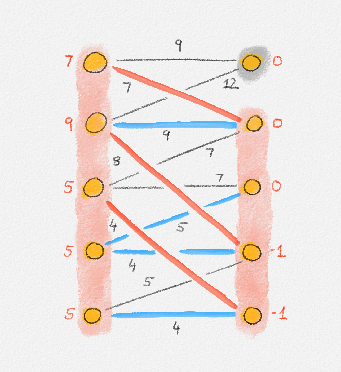
Figure 7.13: The two bottom vertices on the left side (\(U\)) are unmatched. The vertices shaded pink are the ones in \(X\) and \(Y\), that is, the ones reachable from one of these two vertices via alternating paths. The vertices shaded grey are the ones in \(\bar X\) and \(\bar Y\), that is, the ones not reachable from one of these two vertices via alternating paths. In this example, \(\bar X = \emptyset\). The red edges are in the current matching. The blue edges are unmatched edges in \(F^\pi\). In particular, they are tight. The black edges are not in \(F^\pi\). In this example, none of the black edges is tight. In general, however, there can be tight edges that are not included in \(F^\pi\).

Let

\[\delta = \min_{u \in X, w \in \bar Y} (c_{u,w} - \pi_u - \pi_w),\]

and define a new potential function \(\pi'\) as

\[\pi_v' = \begin{cases} \pi_v + \delta & \text{if } v \in X\\ \pi_v - \delta & \text{if } v \in Y\\ \pi_v & \text{otherwise}. \end{cases}\]

We replace our potential function \(\pi\) with \(\pi'\) and then start another iteration. As we will show next, every edge in \(M\) remains tight with respect to this new potential function \(\pi'\), and the alternating forest \(F^{\pi'}\) contains all vertices in \(Y\) as well as at least one vertex in \(\bar Y\). Thus, after adjusting \(\pi\) in this fashion at most \(n\) times, \(F\) contains all vertices in \(W\). As long as the current matching \(M\) is not a perfect matching, there exists an unmatched vertex in \(W\), that is, once \(F^\pi\) contains all vertices in \(W\), there must exist an augmenting path in \(F^\pi\), and this augmenting path is tight. This is the argument why each phase consists of at most \(n\) iterations that adjust \(\pi\) as just described, followed by an iteration that increases the size of \(M\).

Figure 7.14 illustrates a complete run of the Hungarian Algorithm. Note that the graph in Figure 7.14 is not complete. We can apply the Hungarian Algorithm also to incomplete bipartite graphs, only the algorithm is no longer guaranteed to succeed because the graph may not have a perfect matching.

Phase 1

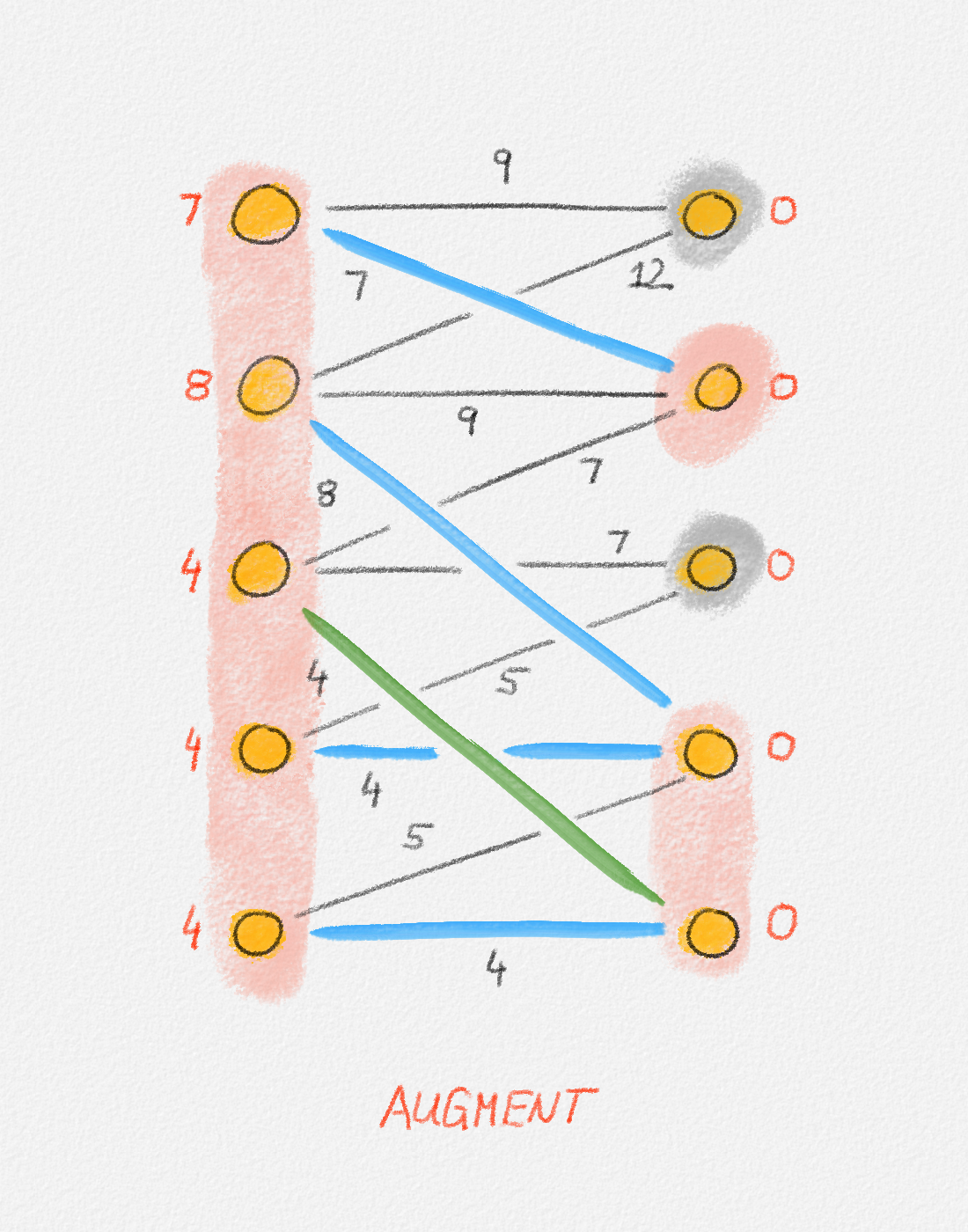
Phase 2

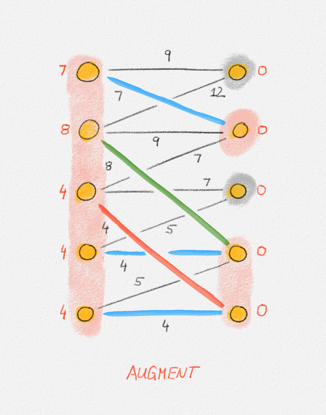
Phase 3

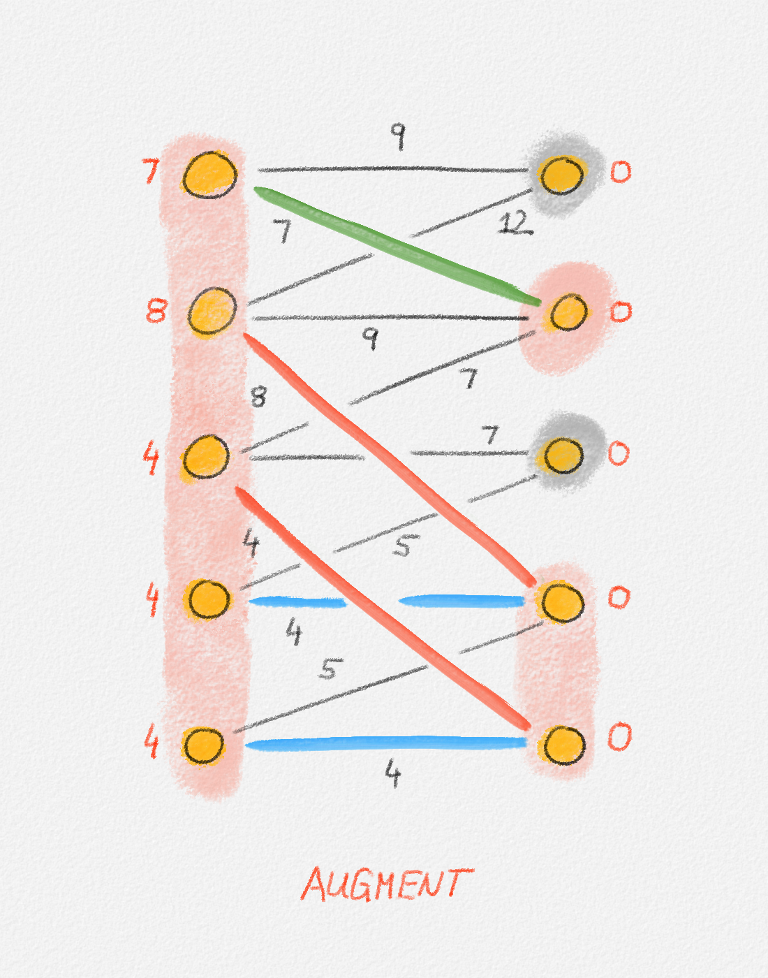
Phase 4

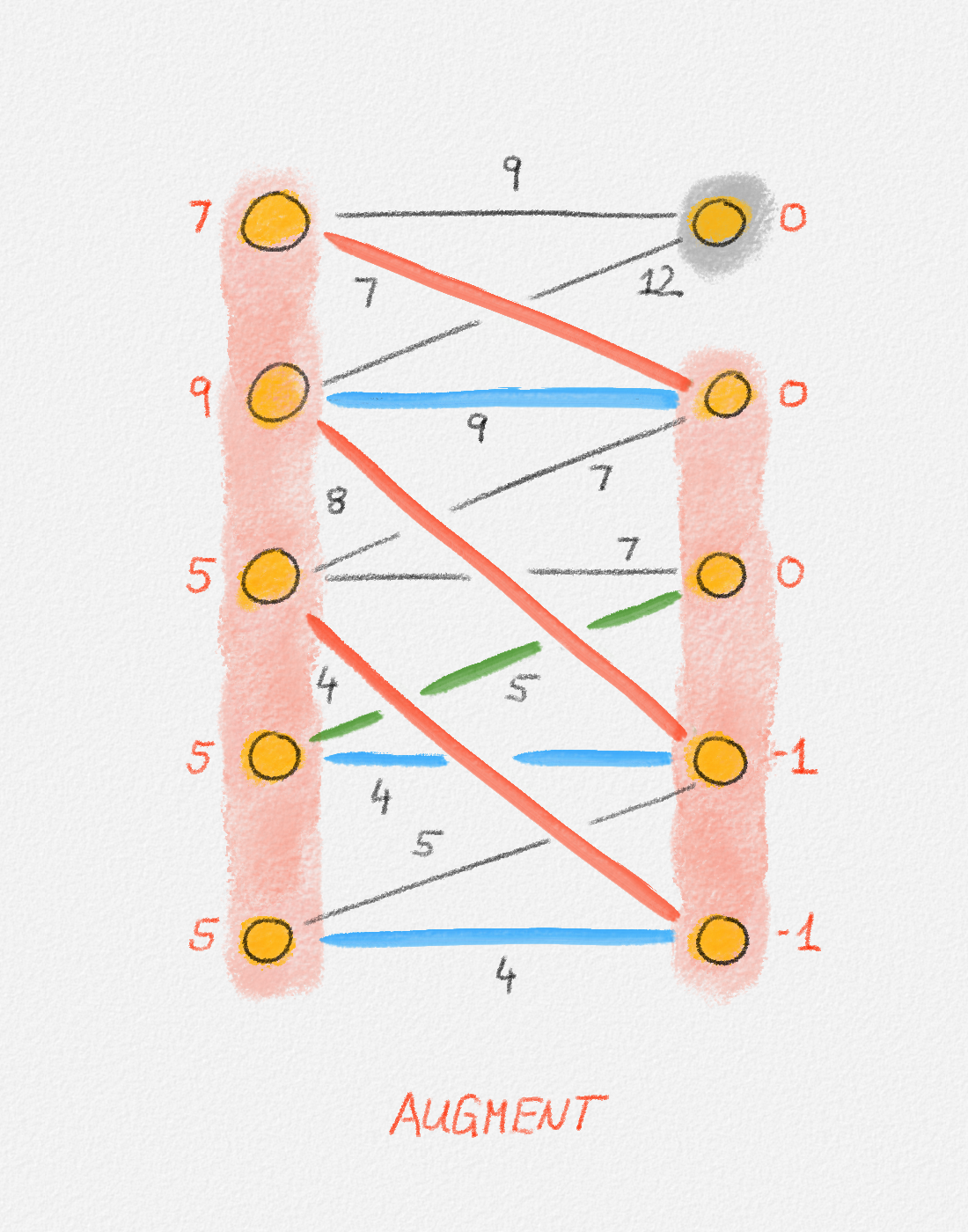
Phase 5

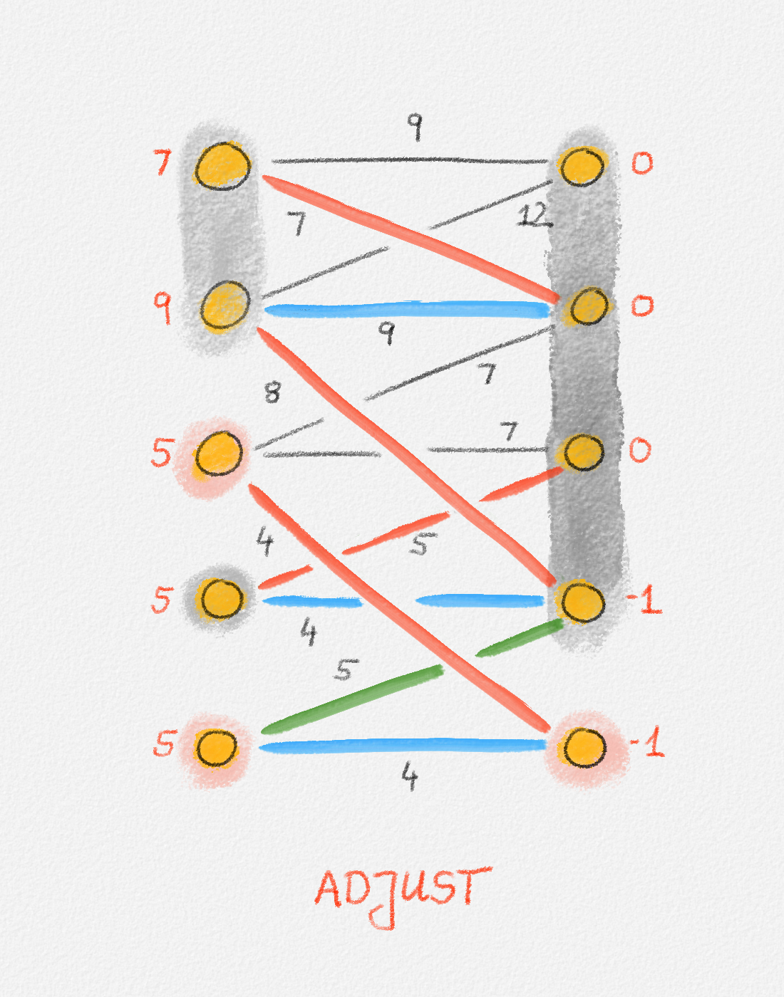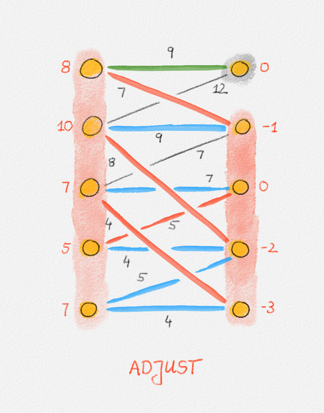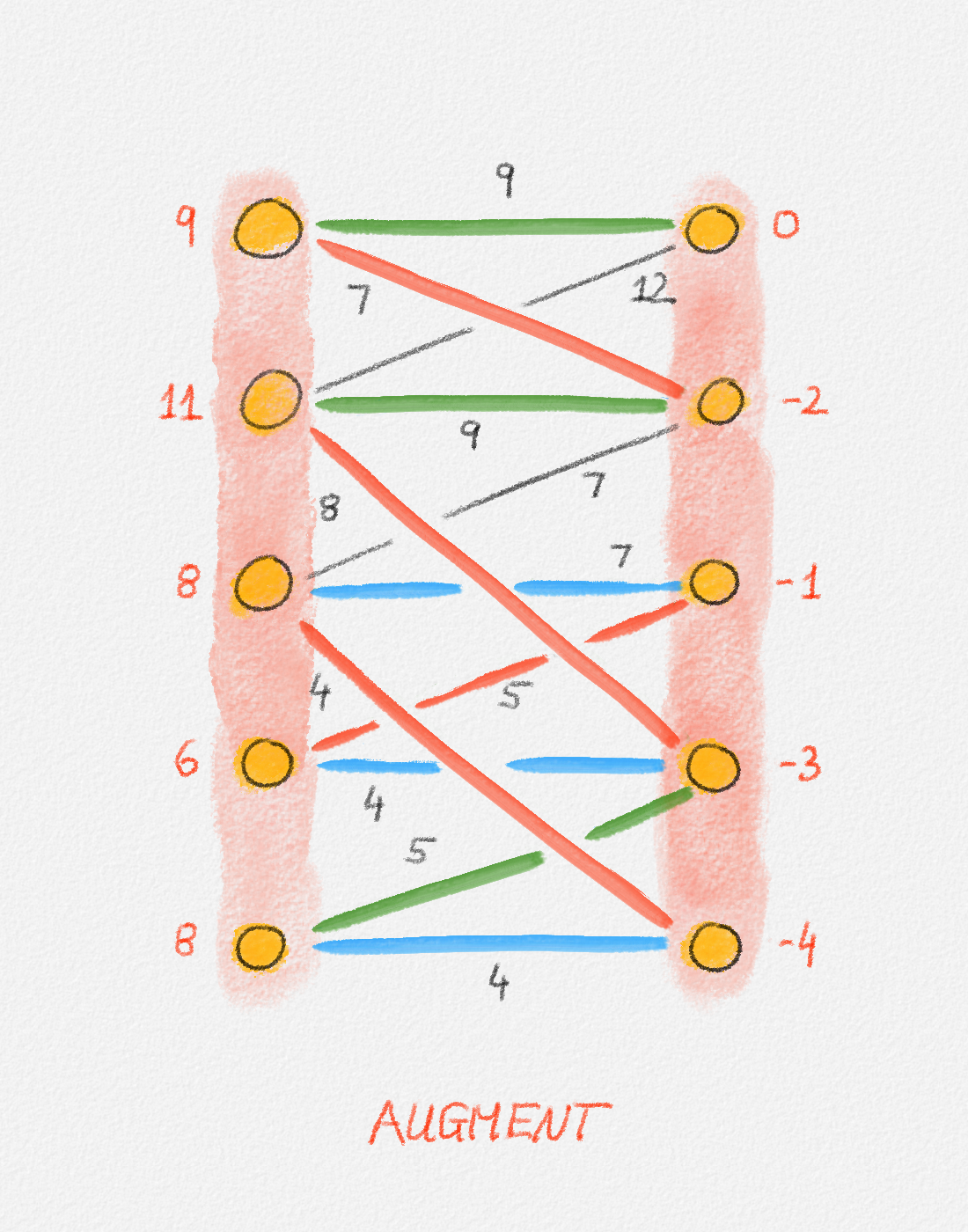Final matching

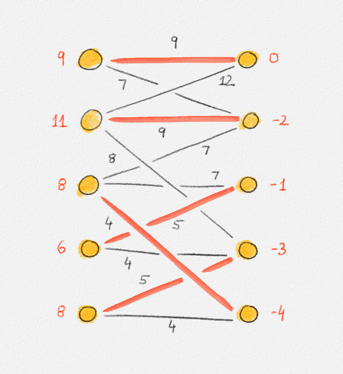
Figure 7.14: Illustration of a full run of the Hungarian algorithm. In this case, the algorithm runs for 5 phases. The final iteration in each phase grows the matching. If the phase has more than one iteration, the iterations before the final iteration adjust the potential function to create more tight edges that can be followed to obtain a larger alternating forest \(F^\pi\). In each figure, red vertex labels are the vertex potentials. Black edge labels are the edge costs. \(X\) and \(Y\) are shaded pink. \(\bar X\) and \(\bar Y\) are shaded grey. Blue edges are tight, black edges are not. Red edges are the edges in the current matching and are also tight. In an augmentation iteration, the augmenting path used to grow the matching is the one composed of the green edges and possibly red matching edges connecting them. (The only phase in this example where the augmenting path has more than one edge is Phase 5.) In an adjustment iteration, the green edge is the tightest edge between \(X\) and \(\bar Y\). The vertex potentials of the vertices in \(X\) and \(Y\) are adjusted by the slack of this edge. The last figure shows the final matching and potential function computed by the algorithm. The matching is clearly a perfect matching. The potential function is a valid potential function and all edges in the matching are tight with respect to this potential function, so the matching is a minimum-weight perfect matching.

7.5.2.2. Correctness of Each Iteration

We already argued that the matching \(M \oplus P_w\) produced by an iteration that finds an augmenting path is \(F^\pi\) is once again composed of only tight edges. Thus, each such iteration maintains complementary slackness.

Next we prove that every edge in \(M\) remains tight with respect to the potential function

\[\pi_v' = \begin{cases} \pi_v + \delta & \text{if } v \in X\\ \pi_v - \delta & \text{if } v \in Y\\ \pi_v & \text{otherwise}, \end{cases}\]

where \(X\) and \(Y\) are the subsets of vertices in \(U\) and \(W\), respectively, that belong to \(F^\pi\), \(\bar X = U \setminus X\), and \(\bar Y = W \setminus Y\), and

\[\delta = \min_{u \in X, w \in \bar Y}(c_{u,w} - \pi_u - \pi_w).\]

We also prove that \(|Y'| > |Y|\), where \(X'\) and \(Y'\) are the subsets of vertices in \(U\) and \(W\), respectively, that belong to \(F^{\pi'}\), \(\bar X' = U \setminus X'\), and \(\bar Y' = W \setminus Y'\). Thus, it takes at most \(n\) iterations to include all vertices in \(W\) in \(F^\pi\), at which point we are guaranteed to find an augmenting path to grow \(M\), unless \(M\) is already a perfect matching.

Lemma 7.18: If the potential function \(\pi\) is feasible and every edge in \(M\) is tight with respect to \(\pi\), then \(\pi'\) is feasible and every edge in \(M\) is tight with respect to \(\pi'\).

Proof: First observe that \(\delta \ge 0\) because \(\pi\) is a feasible potential function, that is, every edge \((u,w) \in E\) satisfies \(c_{u,w} - \pi_u - \pi_w \ge 0\).

Since we have \(\pi_w \le 0\) and \(\pi'_w = \pi_w\) or \(\pi'_w = \pi_w - \delta\) for every vertex \(w \in W\), this immediately implies that \(\pi'_w \le 0\) for every vertex \(w \in W\).

Next observe that every edge \((u,w) \in E\) satisfies

\[\bigl(\pi'_u + \pi'_w\bigr) - (\pi_u + \pi_w) = \begin{cases} \hphantom{-}\delta & \text{if } u \in X \text{ and } w \in \bar Y\\ -\delta & \text{if } u \in \bar X \text{ and } w \in Y\\ \hphantom{-}0 & \text{otherwise}. \end{cases}\tag{7.9}\]

Thus, unless \(u \in X\) and \(w \in \bar Y\), we have \(\pi'_u + \pi'_w \le \pi_u + \pi_w \le c_{u,w}\). If \(u \in X\) and \(w \in \bar Y\), then, by the choice of \(\delta\), we have \(\pi'_u + \pi'_w = \pi_u + \pi_w + \delta \le \pi_u + \pi_w + (c_{u,w} - \pi_u - \pi_w) = c_{u,w}\).

Since \(\pi_w' \le 0\) for all \(w \in W\) and \(\pi_u' + \pi_w' \le c_{u,w}\) for all \((u,w) \in E\), \(\pi'\) is a feasible potential function.

By the next lemma, each edge \((u,w) \in M\) satisfies \(u \in X\) and \(w \in Y\) or \(u \in \bar X\) and \(w \in \bar Y\). Thus, by (7.9), \(\pi_u' + \pi_w' = \pi_u + \pi_w\). Since every edge in \(M\) is tight with respect to \(\pi\), it is therefore also tight with respect to \(\pi\). ▨

Lemma 7.19: Every edge \((u,w) \in M\) satisfies \(u \in X\) if and only if \(w \in Y\).

Proof: Assume that \(u \in X\). Then there exists a tight alternating path \(P\) from some unmatched vertex \(u' \in U\) to \(u\). Since \(u \in U\), this path is even, that is, its last edge is in \(M\). Since \((u,w)\) is the only edge in \(M\) incident to \(u\) (\(M\) is a matching), \(w\) must be \(u\)'s predecessor in \(P\) and the subpath of \(P\) from \(u'\) to \(w\) is a tight alternating path from \(u'\) to \(w\). Therefore, \(w \in Y\).

Now assume that \(w \in Y\). Then there exists a tight alternating path \(P\) from some unmatched vertex \(u' \in U\) to \(w\). Since \(w \in W\), this path is odd, that is, its last edge is not in \(M\). Since \((u,w) \in M\), the edge \((u,w)\) is tight. Thus, appending this edge to \(P\) gives a tight alternating path from \(u'\) to \(u\), and \(u \in X\). ▨

Lemma 7.20: The alternating forest \(F^{\pi'}\) with respect to \(\pi'\) contains more vertices from \(W\) than the alternating forest \(F^{\pi}\) with respect to \(\pi\).

Proof: Let \(X\), \(Y\), \(\bar X\), \(\bar Y\), \(X'\), \(Y'\), \(\bar X'\), and \(\bar Y'\) be defined as above. The lemma claims that \(|Y'| > |Y|\). To prove this, it suffices to prove that \(X \subseteq X'\) and \(Y \subset Y'\).

We start by proving that \(X \subseteq X'\) and \(Y \subseteq Y'\). Then we prove that \(Y'\) contains at least one vertex that is not in \(Y\). Thus, \(Y \subset Y'\).

The vertex set of \(F^\pi\) is \(X \cup Y\). Assume that there exists a vertex \(z \in X \cup Y\) that is not in \(F^{\pi'}\). Then choose this vertex so that the length of the path \(P_z\) from \(z\) to \(r_z\) in \(F^{\pi}\) is minimized. Let \(v\) be \(z\)'s predecessor in \(P_z\). By the choice of \(z\), \(v \in F^{\pi'}\). Thus, there exists a tight alternating path \(P'_v\) with respect to \(\pi'\) from an unmatched vertex \(u \in U\) to \(v\). Note that the edge \((v,z)\) is tight with respect to \(\pi\) because it belongs to \(P_z\). Since \(v, z \in F^\pi\), we have either \(v \in X\) and \(z \in Y\) or \(v \in Y\) and \(z \in X\). In both cases, \(\pi'_v + \pi'_z = \pi_v + \pi_z = c_{v,z}\), that is, the edge \((v,z)\) is tight also with respect to \(\pi'\).

Now, if \(z \in U\), then the path \(P_z\) is even, so the edge \((v,z)\) is in \(M\), \(v \in W\), and the path \(P'_v\) is odd. If \(z \in W\), then the path \(P_z\) is odd, so the edge \((v,z)\) is not in \(M\), \(v \in U\), and the path \(P'_v\) is even. In both cases, appending the edge \((v,z)\) to the path \(P'_v\) produces a tight alternating path from \(u\) to \(z\) with respect to \(\pi'\), that is, \(z \in X' \cup Y'\) (unless \(z \in P'_v\), in which case \(z\) also belongs to \(X' \cup Y'\)), a contradiction. This proves that \(X \cup Y \subseteq X' \cup Y'\), that is, \(X \subseteq X'\) and \(Y \subseteq Y'\).

Next consider any edge \((u,w)\) such that \(u \in X\), \(w \in \bar Y\), and \(c_{u,w} - \pi_u - \pi_w = \delta\). By the definition of \(\delta\), such an edge exists. This edge satisfies \(\pi'_u + \pi'_w = \pi_u + \pi_w + \delta = \pi_u + \pi_w + (c_{u,w} - \pi_u - \pi_w) = c_{u,w}\), that is, this edge is tight with respect to \(\pi'\). Since \(u \in X\) and \(X \subseteq X'\), there exists a tight alternating path \(P'_u\) with respect to \(\pi'\) from some unmatched vertex \(u' \in U\) to \(u\). Since \(u \in U\), this path is even and therefore ends in an edge in \(M\). By Lemma 7.19, \((u,w) \notin M\). Thus, the path obtained by appending the edge \((u,w)\) to \(P'_u\) is a tight alternating path from \(u'\) to \(w\) with respect to \(\pi'\), that is, \(w \in Y'\). Since \(w \in \bar Y\), this shows that \(Y \subset Y'\). ▨

7.5.2.3. Summary of the Algorithm

Let us summarize how the Hungarian algorithm works.

We start with an empty matching \(M = \emptyset\) and a feasible potential function \(\pi\). This choice guarantees that complementary slackness holds initially.

Then each iteration either finds a tight augmenting path \(P\) composed of tight edges, or it replaces \(\pi\) with a new potential function \(\pi'\) such that \(F^{\pi'}\) includes more vertices in \(W\) than \(F^\pi\) does and all edges in \(M\) remain tight with respect to \(\pi'\). We can do the latter at most \(n\) times before we are guaranteed to find a tight augmenting path in \(F^\pi\). Thus, each phase has at most \(n + 1\) iterations. Since the algorithm needs \(n\) phases to arrive at a perfect matching, it terminates after \(O\bigl(n^2\bigr)\) iterations. Since we maintain complementary slackness at all times, the final matching is in fact a minimum-weight perfect matching.

To bound the running time of the algorithm by \(O\bigl(n^4\bigr)\), it suffices to prove that each iteration takes \(O\bigl(n^2\bigr)\) time.

Observe that it takes \(O(n + m) = O\bigl(n^2\bigr)\) time to identify the current tight subgraph \(G^\pi\) of \(G\) and find an alternating forest \(F^\pi\) of \(G^\pi\). If \(F^\pi\) contains an unmatched vertex \(w \in W\), it takes \(O(n)\) extra time to trace the path \(P_w\) in \(F^\pi\) from \(w\) to \(r_w\) and augment \(M\) with \(P_w\). Thus, the last iteration of each phase takes \(O\bigl(n^2\bigr)\) time.

If \(F^\pi\) contains no unmatched vertex in \(W\), then it takes \(O\bigl(n^2\bigr)\) time to inspect all edges between vertices in \(X\) and vertices in \(\bar Y\) to determine \(\delta\) and \(O(n)\) additional time to add \(\delta\) to the potential of every vertex in \(X\) and subtract \(\delta\) from the potential of every vertex in \(Y\). Thus, any iteration that is not the last iteration in its phase also takes \(O\bigl(n^2\bigr)\) time.

Since the algorithm runs for at most \(n^2 + n\) iterations and each iteration takes \(O\bigl(n^2\bigr)\) time, the algorithm runs in \(O\bigl(n^4\bigr)\) time. Thus, we obtain the following result:

Theorem 7.21: The Hungarian Algorithm takes \(O\bigl(n^4\bigr)\) time to find a minimum-weight perfect matching in a complete bipartite graph \(G = (U, W, E)\) with \(|U| = |W| = n\).

7.5.3. A Faster Implementation*

Our goal in this section is to reduce the running time of the Hungarian Algorithm to \(O\bigl(n^3\bigr)\). We do not change the basic algorithm at all: Each iteration computes an alternating forest and uses it to either find a tight augmenting path for \(M\) or update \(\pi\) so that more vertices in \(W\) are reachable from unmatched vertices in \(U\) via tight alternating paths.

The key to reducing the running time of the algorithm to \(O\bigl(n^3\bigr)\) is to reduce the running time of each iteration to \(O(n)\).

The main steps that each iteration performs are

1. Construct an alternating forest \(F^\pi\) and the sets \(X\), \(Y\), \(\bar X\), and \(\bar Y\).
2. Trace an augmenting path in \(F^\pi\) and augment the matching (if there exists an unmatched vertex in \(Y\)).
3. Compute \(\delta\) (if all vertices in \(Y\) are unmatched).
4. Update \(\pi\) (if all vertices in \(Y\) are unmatched).

Steps 2 and 4 already take \(O(n)\) time. Steps 1 and 3 are the ones that take quadratic time. To reduce their cost to \(O(n)\) per iteration, we observe that neither \(F_\pi\) nor \(\delta\) needs to be computed from scratch in each iteration. We do need to compute them from scratch in each phase, every time the matching \(M\) changes. However, updating \(\pi\) only grows \(X\) and \(Y\), as shown in the proof of Lemma 7.20. The proof of Lemma 7.18 shows that every edge in \(F^\pi\) remains tight when we update \(\pi\) (because its endpoints are in \(X\) and \(Y\)). Thus, instead of recomputing \(F^\pi\) in each iteration, we simply add to the forest \(F^\pi\) from the previous iteration, and we update \(\delta\) in the process to maintain that it is the minimum slack of the edges between \(X\) and \(\bar Y\).

An elegant implementation of this idea embeds the adjustment of \(\pi\) directly into the construction of \(F^\pi\). The construction of \(F^\pi\) proceeds in up to \(2n\) iterations, during which the algorithm maintains the following information:

• Every vertex \(z \in X \cup Y\) stores its parent \(p_z\) in \(F^\pi\). Any unmatched vertex \(u \in U\) satisfies \(p_u = \textrm{NULL}\). We use these parent pointers to trace an augmenting path \(P_w\) at the end of the phase, as soon as we discover an unmatched vertex \(w\) in \(F^\pi\).

• Every vertex \(w \in \bar Y\) also stores a "parent" \(p_w\). This is the vertex \(p_w \in X\) such that \(c_{p_w,w} - \pi_{p_w} - \pi_w = \min_{u \in X} (c_{u,w} - \pi_u - \pi_w)\). In other words, \(p_w\) is the other endpoint of the edge with minimum slack among all edges connecting \(w\) to a vertex in \(X\). For \(w \in \bar Y\), \((p_w,w)\) is not an edge in \(F^\pi\) yet. Think about \(p_w\) as the vertex that becomes \(w\)'s parent in \(F^\pi\) once we raise \(\pi_{p_w}\) sufficiently.

• Every vertex \(w \in \bar Y\) stores its slack \(\delta_w = \min_{u \in X}(c_{u,w} - \pi_u - \pi_w)\). This is exactly the slack of the edge \((p_w, w)\).

• We store the overall slack \(\delta = \min_{w \in \bar Y} \delta_w\). Note that this is exactly the value \(\delta\) we use to adjust \(\pi\), only we now maintain \(\delta\) as we change \(F^\pi\) instead of computing it from scratch when we cannot grow \(F^\pi\) anymore.

The construction of \(F^\pi\) maintains the sets \(X\), \(Y\), \(\bar X\), and \(\bar Y\) explicitly. Initially, \(X\) contains all unmatched vertices in \(U\), \(\bar X = U \setminus X\), \(Y = \emptyset\), and \(\bar Y = W\). This corresponds to initializing the queue of the alternating BFS with the unmatched vertices in \(U\), but we do not explicitly maintain this queue and may not discover the vertices in \(F^\pi\) in breadth-first order. With this initial definition of \(X\), \(Y\), \(\bar X\), and \(\bar Y\), we initialize parent pointers by setting \(p_u = \textrm{NULL}\) for all \(u \in U\). For every vertex \(w \in W = \bar Y\), we set \(\delta_w = \min_{u \in X} (c_{u,w} - \pi_u - \pi_w)\) and \(p_w = \textrm{argmin}_{u \in X} (c_{u,w} - \pi_u - \pi_w)\). We set \(\delta = \min_{w \in W} \delta_w\). This initialization is easily seen to take \(O\bigl(n^2\bigr)\) time. Since we perform it only once per phase, these initialization steps take \(O\bigl(n^3\bigr)\) time across all \(n\) phases of the algorithm.

Now, as long as \(Y\) does not contain any unmatched vertex, we repeat the following steps:

• If \(\delta = 0\), then there exists a vertex \(w \in \bar Y\) with \(\delta_w = 0\), that is, the edge \((p_w, w)\) is tight. We add \(w\) and the edge \((p_w, w)\) to \(F^\pi\), by moving \(w\) from \(\bar Y\) to \(Y\).

  • If \(w\) is unmatched, then \(F^\pi\) now contains an unmatched vertex in \(W\). The construction of \(F^\pi\) ends and the phase concludes by replacing \(M\) with \(M \oplus P_w\).

  • If \(w\) is matched to a vertex \(u \in U\), then \(u \in \bar X\) because we always add mates to \(F^\pi\) together. In this case, we set \(p_u = w\) and add \(u\) and the edge \((p_u, u)\) to \(F_\pi\) by moving \(u\) from \(\bar X\) to \(X\). This makes \(u\) a new neighbour in \(X\) of every vertex \(w' \in \bar Y\), so we update the slack of \(w'\) to \(\delta_{w'} = \min(\delta_{w'}, c_{u,w'} - \pi_u - \pi_{w'})\) and set \(p_{w'} = u\) if \(\delta_{w'} = c_{u,w'} - \pi_u - \pi_{w'}\) now. Finally, we set \(\delta = \min_{w' \in W} \delta_{w'}\) and proceed to the next iteration.

  Note that moving \(w\) from \(\bar Y\) to \(Y\) and \(u\) from \(\bar X\) to \(X\) is easily accomplished in constant time. Updating the slack values of all vertices in \(\bar Y\) and updating \(\delta\) take constant time per vertex in \(\bar Y\), \(O(n)\) time in total. Thus, the cost of each iteration in which \(\delta = 0\) is \(O(n)\).

• If \(\delta > 0\), we increase \(\pi_u\) by \(\delta\) for every vertex \(u \in X\), decrease \(\pi_w\) by \(\delta\) for every vertex \(w \in Y\), decrease \(\delta_w\) by \(\delta\) for every vertex \(w \in \bar Y\), decrease \(\delta\) by \(\delta\), that is, set \(\delta = 0\), and then proceed to the next iteration. This clearly takes \(O(n)\) time.

  Note that all edges in \(F^\pi\) remain tight after this update of \(\pi\), that increasing \(\pi_u\) by \(\delta\) for all \(u \in X\) does indeed decrease the slack of every vertex \(w \in \bar Y\) by \(\delta\), and that \(\delta\) does indeed become \(0\) as a result. Also, since all vertices in \(X\) have their potentials decreased by \(\delta\), the minimum-slack edge \((p_w, w)\) connecting \(w\) to a vertex \(p_w \in X\) remains the same for every vertex \(w \in \bar Y\). Thus, we do not need to update \(p_w\) for any vertex \(w \in \bar Y\).

We have argued that each iteration takes \(O(n)\) time. Every iteration in which \(\delta = 0\) adds a vertex in \(\bar Y\) to \(Y\), so there can be at most \(n\) such iterations per phase. If \(\delta > 0\), then the iteration sets \(\delta = 0\), so every iteration in which \(\delta > 0\) is followed by an iteration in which \(\delta = 0\), and there are also at most \(n\) iterations in which \(\delta > 0\). Thus, there are at most \(2n\) iterations per phase. Since the cost per iteration is \(O(n)\) and the initialization of each phase takes \(O\bigl(n^2\bigr)\) time, the cost per phase is thus \(O\bigl(n^2\bigr)\). Since the algorithm runs for \(n\) phases, its running time is therefore \(O\bigl(n^3\bigr)\) and we obtain the following result:

Theorem 7.22: A minimum-weight perfect matching in a complete bipartite graph can be computed in \(O\bigl(n^3\bigr)\) time.

7.6. Bipartite Maximum-Weight Matching

We have discussed how to find a maximum-cardinality matching in a bipartite graph and how to find a minimum-weight perfect matching in a complete bipartite graph with the same number of vertices on each side of the bipartition (otherwise, there is no perfect matching). It is time that we turn our attention to the problem of finding a maximum-weight matching in a bipartite graph.

As we will see shortly, this problem reduces to finding a minimum-weight perfect matching in an auxiliary bipartite graph, so we can once again use the Hungarian Algorithm. In its current form, however, this algorithm is not as efficient as we would like. If the graph is complete, then \(O\bigl(n^3\bigr) = O(nm)\), so the Hungarian Algorithm at least matches the running time of the simple \(O(nm)\)-time algorithm for finding a maximum-cardinality matching. If the graph is sparse, on the other hand—\(m = O(n)\)—then \(O(nm) = O\bigl(n^2\bigr)\) and the Hungarian Algorithm takes \(O(n)\) times longer to find a matching than it takes to find a maximum-cardinality matching.

In Section 7.6.1, we show how to reduce the running time of the Hungarian Algorithm to \(O\bigl(n^2 \lg n + nm\bigr)\). In Section 7.6.2, we show how to reduce maximum-weight matching to minimum-weight perfect matching.

Throughout this section, we assume that all edges have finite costs.

7.6.1. An Even Faster Implementation of the Hungarian Algorithm*

The Hungarian Algorithm does not use the fact that the input graph is complete in any way. We even used an incomplete graph to illustrate the algorithm in Figure 7.14. Completeness only guarantees that the graph has a perfect matching, provided that \(|U| = |W|\). If we run the algorithm on an incomplete graph, it may fail because there may not exist a perfect matching even if \(|U| = |W|\). Figure 7.15 shows an example. If we want to run the Hungarian algorithm on arbitrary bipartite graphs, we need to include an appropriate test whether there even exists a perfect matching. We will discuss this test in Section 7.6.1.4.

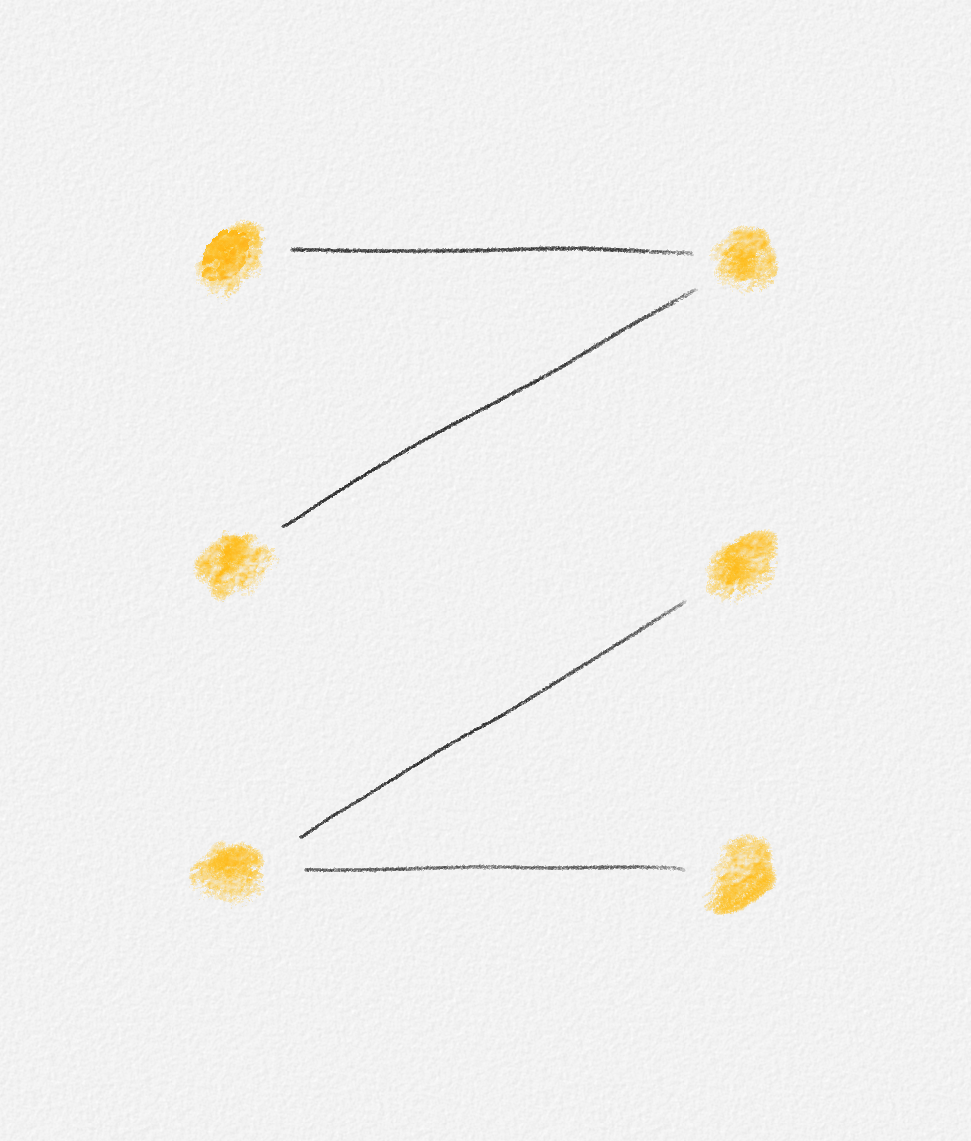
Figure 7.15: A trivial example of a bipartite graph where \(|U| = |W|\) but there is no perfect matching.

The \(O\bigl(n^3\bigr)\) running time of the Hungarian Algorithm in its current form is the result of its running for \(n\) phases, each of which takes \(O\bigl(n^2\bigr)\) time. To reduce the running time of the algorithm to \(O\bigl(n^2\lg n + nm\bigr)\), we show how to reduce the cost per phase to \(O(n \lg n + m)\).

We will show that the initialization of each phase already takes \(O(n + m)\) time. The looser \(O\bigl(n^2\bigr)\) bound on its cost that we obtained before was the result of us not being careful enough in the analysis.¹

The more challenging part is to reduce the cost of all up to \(2n\) iterations in each phase to \(O(n \lg n + m)\). To do this, we show that the last iteration in each phase can be implemented in \(O(n)\) time, and any other iteration can be implemented in \(O(\lg n + \deg(u))\) time, where \(u\) and \(w\) are the vertices moved from \(\bar X\) and \(\bar Y\) to \(X\) and \(Y\) in this iteration. Note that this means that the average cost per iteration is sublinear in \(n\) if \(G\) is sparse. This is something we can achieve only by using appropriate data structures, a priority queue in this case. The initialization of each phase needs to be modified to initialize the priority queue, but this does not increase its cost above \(O(n + m)\).

In Section 7.6.1.1, we start by discussing the data structures we maintain. Then, in Section 7.6.1.2, we discuss the initialization phase and its cost. In Section 7.6.1.3, we show how each iteration, except the last, can be implemented in \(O(\lg n + \deg(u))\) time, and that the last iteration can be implemented in \(O(n)\) time. Section 7.6.1.4 discusses how we detect that no perfect matching exists, so we can abort the algorithm in this case. Finally, Section 7.6.1.5 puts all the pieces together to obtain the fastest version of the Hungarian algorithm we discuss in these notes.

7.6.1.1. The Necessary Data Structures

Recall that each iteration of the Hungarian algorithm finds the vertex \(w \in \bar Y\) with minimum slack \(\delta_w\), moves it to \(Y\) and moves its mate from \(\bar X\) to \(X\) if \(w\) has a mate (is matched). The first thing we need to do to achieve a sublinear cost per iteration is to avoid inspecting all vertices in \(\bar Y\) to find the one with minimum slack. We do this by maintaining a priority queue \(Q\) storing the vertices in \(\bar Y\), ordered by their current slack values \(\delta_w\). This allows us to find the vertex with minimum slack \(\delta_w\) in constant time using a FindMin operation.

When moving a vertex \(u\) from \(\bar X\) to \(X\) and when updating \(\pi\), we also need to update the slack values of the vertices in \(\bar
Y\). Moving a vertex \(u\) from \(\bar X\) to \(X\) does not pose any problems: Given the right priority queue implementation—for example, a Fibonacci Heap or Thin Heap—the DecreaseKey operation necessary to update the priority of every vertex in \(\bar Y\) as a result of having a new neighbour \(u\) in \(X\) takes constant amortized time. Thus, the amortized cost of moving a vertex from \(\bar X\) to \(X\) is \(O(\deg(u))\) (because only the priorities of neighbours of \(u\) need to be updated), which is within the cost per iteration we aim to achieve.

Updating \(\pi\) seems to pose a greater challenge because raising \(\pi_u\) by \(\delta\) for every vertex \(u \in X\) decreases \(\delta_w\) by \(\delta\) for every vertex \(w \in \bar Y\). Thus, if we wanted to maintain the invariant that the priority in \(Q\) of every vertex in \(\bar Y\) is its slack \(\delta_w\), then the cost of updating \(\pi\) would be \(\Omega(|Y|)\), which could be linear in \(n\). To avoid this, observe that I was careful in phrasing what \(Q\) stores above: I said that \(Q\) stores the vertices in \(\bar Y\) ordered by their slack values. I didn't say that their priorities are the slack values. Note that when we increase \(\pi_u\) by \(\delta\) for every vertex \(u \in X\), the slack value \(\delta_w\) changes by the same amount \(\delta\) for every vertex \(w \in \bar Y\). Thus, the relative ordering of the vertices in \(\bar Y\) with respect to their slack values does not change. As a result, we do not need to update any priorities in \(Q\) if all we want to guarantee is that the vertices in \(Q\) are ordered by their slack values. To be able to reconstruct each vertex's slack value from its priority in \(Q\), we maintain a slack adjustment \(\delta_0\), which has the property that the slack of every vertex \(w \in \bar Y\) is its priority in \(Q\) minus this slack adjustment. By adding \(\delta\) to \(\delta_0\), we can (implicitly) decrease the slack values of all vertices \(w \in \bar Y\) by \(\delta\) in constant time.

Let's put the bits and pieces together and give a complete list of the data structures the algorithm maintains:

• For every vertex \(z \in X \cup Y\), we store its parent \(p_z\) in \(F^\pi\), just as in the \(O\bigl(n^3\bigr)\)-time version of the Hungarian algorithm. For every unmatched vertex \(u \in U\), its parent is \(p_u = \textrm{NULL}\).

• For every vertex \(w \in \bar Y\), we store its "parent" \(p_w\), which is the vertex \(p_w \in X\) such that the edge \((p_w, w)\) has minimum slack among all edges connecting \(w\) to a vertex in \(X\). As in the \(O\bigl(n^3\bigr)\)-time version of the Hungarian algorithm, \(p_w\) is the vertex that becomes \(w\)'s parent in \(F^\pi\) once we move \(w\) to \(Y\).

• We store a slack adjustment \(\delta_0\), a single real number.

• We store an adjusted potential \(\pi'_z\) for every vertex \(z \in U \cup W\). Invariant 7.23 below states how the potential \(\pi_z\) of each vertex \(z \in U \cup W\) can be computed in constant time from \(\pi'_z\) and the slack adjustmest \(\delta_0\).

• We maintain a priority queue \(Q\) storing all vertices in \(\bar Y\). Let \(q_w\) be the priority of each vertex \(w \in Q\).

To use these data structures to implement the Hungarian algorithm, we maintain the following invariant:

Invariant 7.23:

• For every vertex \(z \in \bar X \cup \bar Y\), its potential \(\pi_z\) equals \(\pi'_z\).
• For every vertex \(u \in X\), its potential \(\pi_u\) is \(\pi_u' + \delta_0\).
• For every vertex \(w \in Y\), its potential \(\pi_w\) is \(\pi_w' - \delta_0\).
• For every vertex \(w \in \bar Y\), its slack is \(\delta_w = q_w - \delta_0\).

7.6.1.2. Initialization of Each Phase

The initialization of each phase looks very similar to that of the \(O\bigl(n^3\bigr)\)-time implementation of the Hungarian algorithm:

• We start by setting \(\pi'_z = \pi_z\) for every vertex \(z \in U \cup W\) and setting \(\delta_0 = 0\). This establishes the invariants that \(\pi_z = \pi'_z\) for every vertex \(z \in \bar X \cup \bar Y\), \(\pi_u = \pi'_u + \delta_0\) for every vertex \(u \in X\), and \(\pi_w = \pi'_w - \delta_0\) for every vertex \(w \in Y\), no matter how we choose \(X\), \(Y\), \(\bar X\), and \(\bar Y\).

• As in the \(O\bigl(n^3\bigr)\)-time implementation of the Hungarian algorithm, we choose \(X\) to be the set of all unmatched vertices in \(U\), \(\bar X = U \setminus X\), \(Y = \emptyset\), and accordingly, \(\bar Y = W\). For each vertex \(u \in U\), we set \(p_u = \textrm{NULL}\). For each vertex \(w \in \bar Y\), we set \(p_w = \textrm{argmin}_{u \in X}(c_{u,w} - \pi_u - \pi_w)\). This establishes the correct parent pointers for all vertices in \(G\).

• Finally, we calculate \(\delta_w = \min (\{\infty\} \cup \{c_{u,w} - \pi_u - \pi_w \mid (u, w) \in E, u \in X\})\) for every vertex \(w \in \bar Y\) and insert \(w\) into \(Q\) with priority \(q_w = \delta_w\). Since \(\delta_0 = 0\), this establishes the invariant that \(\delta_w = q_w - \delta_0\) for every vertex \(w \in \bar Y\). Note that \(\delta_w = \infty\) if \(w\) has no neighbour in \(X\).

After this initialization, Invariant 7.23 holds.

The cost of the initialization is easily seen to be \(O(n + m)\): Initializing \(\delta_0\) and the adjusted potentials of all vertices in \(G\) takes \(O(n)\) time, as does initializing the parent pointers of all vertices not in \(\bar Y\). Computing \(q_w\) and \(p_w\) for each vertex \(w \in \bar Y\) takes \(O(\deg(w))\) time because it requires inspecting each edge incident to \(w\). Since there are \(m\) edges in \(G\), this takes \(O(m)\) time. If we use a Fibonacci Heap or Thin Heap as the priority queue implementation, then inserting each vertex \(w \in \bar Y\) into \(Q\), with priority \(q_w\), takes constant time. Thus, the initialization of the priority queue adds \(O(|Y|) = O(n)\) to the cost of the initialization.

Lemma 7.24: The initialization of each phase of the Hungarian algorithm takes \(O(n + m)\) time and establishes Invariant 7.23.

7.6.1.3. Implementing Each Iteration

Each iteration in a phase now needs to pick the vertex \(w \in \bar Y\) with minimum slack and move it to \(Y\).

By Invariant 7.23, the vertex with minimum slack also has minimum priority in \(Q\). Thus, we can identify \(w\) in constant time using a FindMin operation.

Also by Invariant 7.23, we have \(\delta_w = q_w - \delta_0\), so we can compute \(\delta_w\) in constant time. Note that since \(w\) is the vertex with minimum slack, we have \(\delta_w = \delta\). Next we need to either update \(\pi\) if \(\delta > 0\) or grow \(F^\pi\) if \(\delta = 0\). We will assume for now that \(\delta = \delta_w < \infty\). As we prove in Section 7.6.1.4, if \(\delta_w = \infty\), then there does not exist a perfect matching in \(G\), so this is how we detect that there exists no perfect matching and abort the algorithm in this case.

Updating \(\boldsymbol{\pi}\)

If \(\delta > 0\), then we need to

• Increase \(\pi_u\) by \(\delta\) for every vertex \(u \in X\),
• Decrease \(\pi_w\) by \(\delta\) for every vertex \(w \in Y\), and
• Decrease \(\delta_{w'}\) by \(\delta\) for every vertex \(w' \in \bar Y\).

We can do this in constant time by adding \(\delta\) to \(\delta_0\). Indeed, by Invariant 7.23, we have

• \(\pi_u = \pi'_u + \delta_0\) for every vertex \(u \in X\). Increasing \(\delta_0\) by \(\delta\) without changing \(\pi'_u\) thus increases \(\pi_u\) by \(\delta\).

• \(\pi_{w'} = \pi'_{w'} - \delta_0\) for every vertex \(w' \in Y\). Increasing \(\delta_0\) by \(\delta\) without changing \(\pi'_{w'}\) thus decreases \(\pi_{w'}\) by \(\delta\).

• \(\delta_{w'} = q_{w'} - \delta_0\) for every vertex \(w' \in \bar Y\). Increasing \(\delta_0\) by \(\delta\) without changing \(q_{w'}\) thus decreases \(\delta_{w'}\) by \(\delta\).

Growing \(\boldsymbol{F^{\pi}}\)

As in the \(O\bigl(n^3\bigr)\)-time implementation of the Hungarian algorithm, we start by moving \(w\) from \(\bar Y\) to \(Y\). This no longer takes constant time, because we need to maintain our data structures and Invariant 7.23, but we can implement this step in \(O(\lg n)\) time:

• First we remove \(w\) from \(Q\) using a DeleteMin operation. This is what takes \(O(\lg n)\) time. Since \(Q\) is our representation of \(\bar Y\), this removes \(w\) from \(\bar Y\) and, thus, adds it to \(Y\).

• To restore Invariant 7.23, we need to update \(\pi'_w\) so that \(\pi_w = \pi'_w - \delta_0\). Since we just removed \(w\) from \(\bar Y\), we currently have \(\pi_w' = \pi_w\). Thus, we ensure that \(\pi_w = \pi'_w - \delta_0\) by increasing \(\pi'_w\) by \(\delta_0\). This clearly takes constant time.

The next steps depend on whether \(w\) is matched.

If \(w\) is unmatched, we have created a tight augmenting path \(P_w\) in \(F^\pi\), and this is the last iteration of the current phase. Note that our data structures do not help us to reduce the cost of reporting \(P_w\) to less than \(O(n)\). However, since this is the last iteration of the phase, we incur this \(O(n)\) cost only once per phase. Since the initialization of the phase already takes \(O(n + m)\) time, adding an \(O(n)\) cost to report the path \(P_w\) to the overall cost of the phase increases the cost of the phase by at most a constant factor.

If \(w\) is matched, then we need to move \(w\)'s mate \(u\) from \(\bar X\) to \(X\) and update the priorities of its neighbours in \(\bar Y\) accordingly:

• First we set \(p_u = w\), thereby making \(u\) the child of \(w\) in \(F^\pi\). This clearly takes constant time.

• Next we restore the part of Invariant 7.23 that states that every vertex \(u' \in X\) has potential \(\pi_{u'} = \pi'_{u'} + \delta_0\). All vertices in \(X \setminus \{u\}\) already satisfy this invariant. To ensure that \(u\) satisfies the invariant, observe that we just removed \(u\) from \(\bar X\). Thus, by Invariant 7.23, we have \(\pi'_u = \pi_u\). By decreasing \(\pi'_u\) by \(\delta_0\), we establish the condition that \(\pi_u = \pi'_u + \delta_0\). This clearly takes constant time.

• Finally, we restore the invariant that the slack of every vertex \(w' \in \bar Y\) is \(\delta_{w'} = q_{w'} - \delta_0\). Note that moving \(u\) from \(\bar X\) to \(X\) leaves the slack of \(w'\) unchanged if \((u, w') \notin E\). If \((u, w') \in E\), then the new slack of \(w'\) is \(\delta_{w'} = \min(\delta_{w'}, c_{u,w'} - \pi_u - \pi_{w'})\).

  By Invariant 7.23, we can compute the current slack \(\delta_{w'}\) of \(w'\) by subtracting \(\delta_0\) from the current priority \(q_{w'}\) of \(w'\). We can also compute \(\pi_u\) as \(\pi'_u + \delta_0\) and \(\pi_{w'}\) as \(\pi'_{w'}\) because \(u \in X\) and \(w' \in \bar Y\). Next we compare \(\delta_{w'}\) with \(c_{u,w'} - \pi_u - \pi_w\).

  If \(\delta_{w'} \le c_{u,w'} - \pi_u - \pi_{w'}\), then the slack of \(w'\) does not change as the result of moving \(u\) from \(\bar X\) to \(X\): the edge \((u, w')\) is not the minimum-slack edge connecting \(w'\) to \(X\). Thus, no further updates of \(w'\) are required.

  If \(\delta_{w'} > c_{u,w'} - \pi_u - \pi_{w'}\), then \((u,w')\) is the new minimum-slack edge connecting \(w'\) to \(X\). We start by setting \(p_{w'} = u\). This takes constant time. Then we need to update \(q_{w'}\) to reflect the decrease of \(\delta_{w'}\). Since Invariant 7.23 requires that \(\delta_{w'} = q_{w'} - \delta_0\) and we now have \(\delta_{w'} = c_{u,w'} - \pi_u - \pi_{w'}\), we need to decrease \(q_{w'}\) to \(c_{u,w'} - \pi_u - \pi_{w'} + \delta_0\), which we do using a DecreaseKey operation. On a Fibonacci Heap or Thin Heap, this operation takes amortized constant time.

We have shown the following lemma:

Lemma 7.25: Each iteration of the Hungarian algorithm updates the potential function \(\pi\), moves a matched vertex \(w\) from \(\bar Y\) to \(Y\) and its mate \(u\) from \(\bar X\) to \(X\), or moves an unmatched vertex \(w\) from \(\bar Y\) to \(Y\) and reports the resulting augmenting path \(P_w\) in \(F^\pi\). In the first case, the iteration takes constant time. In the second case, it takes amortized \(O(\lg n + \deg(u))\) time. In the last case, the iteration takes \(O(n)\) time and is the last iteration of the current phase.

7.6.1.4. Abort When There's No Perfect Matching

The implementation of the Hungarian algorithm discussed so far behaves exactly like the \(O\bigl(n^3\bigr)\)-time implementation of the Hungarian algorithm but uses efficient data structures to reduce the running time to \(O\bigl(n^2\lg n + nm\bigr)\). We will discuss that this is indeed the running time of the algorithm in Section 7.6.1.5. In this section, we address how we detect that \(G\) has no perfect matching whenever this is the case.

As already stated in Section 7.6.1.3, whenever the vertex \(w \in \bar Y\) with minimum slack \(\delta_w\) satisfies \(\delta_w = \infty\), we abort the algorithm and report that \(G\) has no perfect matching. Next we prove that this is correct.

Lemma 7.26: If \(M\) is not a perfect matching, all vertices in \(Y\) are matched, \(\bar Y \ne \emptyset\), and all vertices in \(\bar Y\) have infinite slack, then there is no perfect matching.

Proof: Since we assume that the current matching \(M\) is not a perfect matching, to prove that there is no perfect matching, it suffices to show that \(M\) is a maximum-cardinality matching.

So assume for the sake of contradiction that \(M\) is not a maximum matching. Then there exists an augmenting path \(P\) for \(M\). Since \(G\) is bipartite, \(P\) has an unmatched endpoint \(u \in U\) and an unmatched endpoint \(w \in W\). Since we start the phase by adding all unmatched vertices in \(U\) to \(X\), we have \(u \in X\). Since we assume that all vertices in \(Y\) are matched (otherwise, the phase would end because we have found a tight augmenting path), we have \(w \in \bar Y\). Thus, \(P\) starts in \(X \cup Y\) and ends in \(\bar X \cup \bar Y\). Let \(z\) be the vertex in \(P\) closest to \(u\) that belongs to \(\bar X \cup \bar Y\).

If \(z \in \bar Y\), then by the choice of \(z\), its predecessor \(u'\) in \(P\) belongs to \(X\). Thus, we have a vertex \(z \in \bar Y\) that has a neighbour in \(X\). Since all edge costs are finite, this implies that \(\delta_z < \infty\), a contradiction.

If \(z \in \bar X\), then by the choice of \(z\), its predecessor \(w'\) in \(P\) belongs to \(Y\). Moreover, the subpath of \(P\) from \(u\) to \(z\) is even and the edge \((w', z)\) is in \(M\). Since we move the mate of every vertex \(w' \in Y\) from \(\bar X\) to \(X\) when moving \(w'\) from \(\bar Y\) to \(Y\), we thus have \(z \in X\), again a contradiction.

Thus, there exists no augmenting path for \(M\) and \(M\) is a maximum-cardinality matching. ▨

7.6.1.5. Summary

The implementation of the Hungarian Algorithm discussed in this section moves the same sequence of vertices from \(\bar Y\) to \(Y\) and computes the same vertex potentials and augmenting path in each phase as the \(O\bigl(n^3\bigr)\)-time implementation from Section 7.5.3. Thus, the algorithm computes a minimum-weight perfect matching.

By Lemmas 7.24 and 7.25, the initialization and the final iteration of each phase take \(O(n + m)\) time in total. Any iteration that updates \(\pi\) takes constant time. Any other iteration takes \(O(\lg n + \deg(u))\) time, where \(w\) is the vertex moved from \(\bar Y\) to \(Y\) and \(u\) is \(w\)'s mate, which is moved from \(\bar X\) to \(X\). Since each phase has at most \(2n\) iterations and every vertex in \(U\) is moved from \(\bar X\) to \(X\) at most once per phase, the total cost of the initialization and all iterations in a phase is thus \(O(n \lg n + m)\). Summing this over all \(n\) phases of the algorithm, this gives a running time of \(O\bigl(n^2 \lg n + nm\bigr)\) for the whole algorithm. Thus, we have the following result:

Theorem 7.27: A minimum-weight perfect matching in a bipartite graph \(G\) can be computed in \(O\bigl(n^2 \lg n + nm\bigr)\) time if \(G\) has a perfect matching. If \(G\) has no perfect matching, the algorithm detects this and aborts.

7.6.2. Maximum-Weight Matching

To compute a maximum-weight matching in a bipartite graph \(G\), we first observe that this is the same as computing a minimum-weight matching in \(G\) after negating all edge weights. To compute a minimum-weight matching in \(G\), we reduce this problem to computing a minimum-weight perfect matching in an auxiliary graph \(G''\).

The graph \(G''\) consists of \(G\) and an identical copy \(G'\) of \(G\). In addition, for every vertex \(x \in G\), \(G''\) has an edge \((x,x')\) of weight zero, where \(x'\) is the copy of \(x\) in \(G'\). This is illustrated in Figure 7.16. \(G''\) has a trivial perfect matching \(\{(x,x') \mid x \in G\}\). Since \(G''\) has \(2n\) vertices and \(2m + n\) edges, we can compute a minimum-weight perfect matching \(M''\) of \(G''\) in \(O\bigl(n^2 \lg n + nm\bigr)\) time. By the next lemma, the matching \(M = \{(x,y) \in M'' \mid x,y \in G\}\) is a minimum-weight matching of \(G\).

Figure 7.16: The graph \(G''\) used to compute a minimum-weight matching in \(G\). \(G\) and its copy, \(G'\), are shaded. Note that every edge in \(G'\) has the same cost as the corresponding edge in \(G\). The edge between every vertex in \(G\) and its copy in \(G'\) has cost \(0\). By connecting each vertex in \(G\) to its copy in \(G'\), we obtain a trivial perfect matching of \(G''\).

Lemma 7.28: If \(M''\) is a minimum-weight perfect matching of \(G''\), then the matching \(M = \{(x,y) \in M'' \mid x,y \in G\}\) is a minimum-weight matching of \(G\).

Proof: Let \(M^*\) be a minimum-weight matching of \(G\) and consider the two matchings \(M = \{(x, y) \in M'' \mid x, y \in G\}\) and \(M' = \{(x,y) \in M'' \mid x, y \in G'\}\). Since \(M^*\) is a minimum-weight matching of \(G\), \(M\) is a matching of \(G\), and \(M'\) is a matching of \(G'\), we have \(c(M) \ge c(M^*)\) and \(c(M') \ge c(M^*)\). If \(c(M) > c(M^*)\), then observe that \(c(M'') = c(M) + c(M') > 2c(M^*)\) because every edge between \(G\) and \(G'\) in \(G''\) has weight \(0\). On the other hand, the matching \(M''' = \{(x,y), (x',y') \mid (x,y) \in M^*\} \cup \{(x,x') \mid x \in G \text{ is unmatched by } M^*\}\) is a perfect matching of \(G''\) of weight \(2c(M^*)\). Thus, \(M''\) is not a minimum-weight perfect matching of \(G''\), a contradiction. This shows that \(c(M) \le c(M^*)\). Since \(c(M) \ge c(M^*)\), we therefore have \(c(M) = c(M^*)\), that is, \(M\) is a minimum-weight matching of \(G\). ▨

Note that the reduction from the maximum-weight matching problem to the minimum-weight perfect matching problem discussed in this section works for any graph, not just for bipartite graphs. In order to compute a maximum-weight matching, however, we need an algorithm for computing a minimum-weight perfect matching. We only discussed how to do this for bipartite graphs, so we obtain the following result using Theorem 7.27 and Lemma 7.28:

Theorem 7.29: A maximum-weight matching in a bipartite graph can be computed in \(O\bigl(n^2 \lg n + nm\bigr)\) time.

7.7. General Maximum-Cardinality Matching

The overall strategy of the bipartite maximum matching algorithm in Section 7.4 does not use that the graph is bipartite at all. Indeed, Corollary 7.9 states that a matching is a maximum-cardinality matching if and only if there is no augmenting path; there is no requirement that the graph should be bipartite. Thus, we can find a maximum-cardinality matching in any graph by starting with the empty matching or with a maximal matching and then repeatedly finding augmenting paths and augmenting the matching until no augmenting path exists.

Where bipartiteness is used in the bipartite maximum matching algorithm is in finding an augmenting path efficiently. In a bipartite graph \(G = (U, W, E)\), every augmenting path, having odd length, needs to start at an unmatched vertex in \(U\) and end at an unmatched vertex in \(W\). Alternating BFS from the unmatched vertices in \(U\) allowed us to find such a path in \(O(m)\) time (or to decide that there is no augmenting path and the matching is therefore maximum).

It turns out that finding an augmenting path in an arbitrary undirected graph is significantly harder. The fact that we cannot meaningfully divide the unmatched vertices into two subsets, those in \(U\) and those in \(W\), so that the augmenting path we need to find starts in one of those sets and ends in the other is only a minor nuisance. The more fundamental problem is that non-bipartite graphs can have odd cycles, cycles of odd length. By Exercise 7.2, bipartite graphs do not. Figure 7.17 shows an example where performing BFS or DFS to construct an alternating forest fails to find an augmenting path even though such a path exists. The problem is the highlighted odd cycle.

Figure 7.17: In this example, alternating BFS constructs an alternating forest that includes the path \(\langle a, b, c, d \rangle\). Alternating DFS may construct an alternating forest that includes this path. In any such forest, \(d\) is an odd vertex, so the edge \((d,e)\) is not included in the forest. In particular, the alternating forest does not include the yellow augmenting path. The problem in this example is the odd cycle shaded in pink. In order to discover the yellow augmenting path, we need to make our alternating forest travel around this cycle "in the right direction". This is what makes finding an augmenting path in non-bipartite graphs hard.

• In Section 7.7.1, we discuss Edmonds's algorithm for finding an augmenting path in an arbitrary graph in \(O(nm)\) time. The key strategy of Edmonds's algorithm can be described as follows: It runs alternating BFS from all unmatched vertices. It may then be possible to identify an augmenting path composed of two paths in the constructed alternating forest and an edge that joins them. If the algorithm finds such a path, it returns it. If it does not, then there are two possibilities: Either there is no augmenting path or there must exist a particular type of odd cycle, called a "blossom", composed of a path in the alternating forest plus one edge not in the forest. The algorithm is able to distinguish between these two cases. If there is no augmenting path, then the current matching is maximum and the algorithm exits. If there exists a blossom, the algorithm replaces the entire blossom with a single vertex: It "contracts" the blossom. It then recursively calls itself on the resulting smaller graph. If it fails to find an augmenting path in this smaller graph, then there is no augmenting path in the original graph either. Otherwise, an augmenting path in the original graph can be constructed easily from an augmenting path in the contracted graph. Since this strategy leads to an \(O(nm)\)-time algorithm to find an augmenting path and we can augment any matching at most \(\frac{n}{2}\) times before the matching is a maximum-cardinality matching, this leads to an \(O\bigl(n^2m\bigr)\)-time algorithm for finding a maximum-cardinality matching in an arbitrary graph.

• Just as we were able to reduce the time needed to find a maximum-cardinality matching in a bipartite graph from \(O(nm)\) to \(O\bigl(m\sqrt{n}\bigr)\), there have been numerous papers written on reducing the running time of Edmonds's algorithm to \(O(nm)\) and, by combining the ideas of Edmonds's algorithm with those of the Hopcroft-Karp algorithm for bipartite graphs, even to \(O\bigl(m\sqrt{n}\bigr)\). Even some of the current world-leading experts on matching algorithms find it difficult to fully verify the correctness of those algorithms. Thus, as at least a modest improvement over Edmonds's algorithm, we will discuss Gabow's implementation of Edmonds's algorithm in Section 7.7.2, which takes \(O\bigl(n^3\bigr)\) time. By implementing Gabow's algorithm using clever data structures, its running time can be reduced to \(O(nm \cdot \alpha(n))\), where \(\alpha\) is the inverse of Ackermann's function, a function that is never greater than a very small constant even for astronomical inputs. We will not discuss this faster implementation here.

7.7.1. Edmonds's Algorithm

Let us assume for now that the graph \(G\) for which we want to compute a maximum-cardinality matching is connected. As already said, Edmonds's algorithm uses the same strategy as any other maximum-cardinality matching algorithm: It starts with either the empty matching \(M = \emptyset\) or with a maximal matching \(M\), which can be found in \(O(n + m) = O(m)\) time. Then it repeatedly grows the matching \(M\) by looking for an augmenting path \(P\) and replacing \(M\) with \(M \oplus P\). Once it fails to find an augmenting path \(P\), \(M\) is a maximum-cardinality matching, by Corollary 7.9. We will show that it takes \(O(nm)\) time to find an augmenting path \(P\) in an arbitrary connected graph, or decide that no such path exists. Since we must obtain a maximum-cardinality matching after at most \(\frac{n}{2}\) iterations, we call this algorithm to find an augmenting path at most \(\frac{n}{2}\) times. Thus, we can find a maximum-cardinality matching in a connected graph in \(O\bigl(n^2m\bigr)\) time.

If the input graph is not connected, then we can compute the connected components of the graph in \(O(n + m)\) time and then find maximum-cardinality matchings for all components. The result is clearly a maximum-cardinality matching of the whole graph. If the components are \(G_1, \ldots, G_k\) and \(G_i\) has \(n_i \le n\) vertices and \(m_i\) edges, then \(\sum_{i=1}^k m_i = m\) and the running time of the whole algorithm is

\[\begin{multline} O(n + m) + \sum_{i=1}^k O\bigl(n_i^2m_i\bigr) \le O(n + m) + \sum_{i=1}^k O\bigl(n^2m_i\bigr)\\ = O(n + m) + O\bigl(n^2m\bigr) = O\bigl(n^2m\bigr). \end{multline}\]

Thus, we obtain the following result:

Theorem 7.30: A maximum-cardinality matching in an arbitrary graph \(G\) can be found in \(O\bigl(n^2m\bigr)\) time.

It remains to discuss how to find an augmenting path in a connected graph in \(O(nm)\) time.

7.7.1.1. Finding and Contracting Blossoms

To find an augmenting path for the current matching \(M\), Edmonds's algorithm starts by computing an alternating forest \(F\) of \(G\) with all unmatched vertices in \(G\) as roots.

Recall that we call a vertex odd or even depending on whether its depth in \(F\) is odd or even. The first lemma in this section states a sufficient, but not necessary, condition under which \(M\) is a maximum-cardinality matching:

Lemma 7.31: If there is no unmatched edge \((x,y) \notin F\) such that \(x\) and \(y\) are both even vertices in \(F\), then \(M\) is a maximum-cardinality matching.

Proof: We prove the contrapositive: If \(M\) is not a maximum-cardinality matching, then there must exist an unmatched edge \((x,y)\) such that \(x\) and \(y\) are both even vertices in \(F\).

If \(M\) is not a maximum-cardinality matching, then there exists an augmenting path \(P\) for \(M\). We partition \(P\) into maximal subpaths \(P_0, \ldots, P_{k+1}\) such that each such subpath contains only edges in \(F\). See Figure 7.18.

Figure 7.18: The path shaded in yellow, grey, and green is an augmenting path \(P\). The yellow paths are the subpaths \(P_1, P_2, P_3, P_4, P_5\) of \(P\) that stay within a single tree in \(F\). Note that each of the paths \(P_2, P_3, P_4\) has an odd and an even endpoint. The grey and green edges are the edges in \(P\) that connect the paths \(P_1, P_2, P_3, P_4, P_5\). Of these, the two green edges are edges with two even endpoints.

For \(0 \le i \le k+1\), let \(x_i\) be the first vertex of \(P_i\), and let \(y_i\) be the last vertex of \(P_i\). We prove that \(y_0\) is an even vertex, \(x_{k+1}\) is an even vertex and, for \(1 \le i \le k\), either \(x_i\) or \(y_i\) is an even vertex. Since \(y_0\) is an even vertex, there exists a maximum index \(0 \le i \le k\) such that \(y_i\) is even. If \(i = k\), then \(x_{i+1} = x_{k+1}\) is even. If \(i < k\), then \(y_{i+1}\) is odd, so \(x_{i+1}\) is even. Since \(y_i\) is even and \(x_{i+1}\) is even, the edge \((y_i, x_{i+1})\) is an edge not in \(F\) connecting two even vertices. Since even vertices in \(F\) are matched by edges in \(F\), this edge is unmatched. The lemma follows.

First consider the path \(P_0\). If \(P_0 = \langle x_0 \rangle\), then \(y_0 = x_0\). Since \(x_0\) is unmatched, \(y_0\) is even in this case. If \(P_0 \ne \langle x_0 \rangle\), then \(y_0\) is a matched vertex because \(y_0 \in T_{x_0}\) and \(x_0\) is the only unmatched vertex in \(T_{x_0}\). Since \(y_{k+1}\) is unmatched, this implies that \(y_0 \ne y_{k+1}\), so \(k \ge 0\) and \(y_0\) has a successor \(x_1\) in \(P\). Next observe that \(P_0 = P_{y_0}\) because \(x_0\) is the root of \(T_{x_0}\), \(y_0 \in T_{x_0}\), and all edges in \(P_0\) belong to \(T_{x_0}\). Thus, if \(y_0\) were odd, then the last edge in \(P_0\) would be unmatched. Since \(P\) is an alternating path, this would imply that the edge \((y_0,x_1)\) would have to be matched and \(x_1\) would be in \(T_{x_0}\), a contradiction. This shows that \(y_0\) is even. An analogous argument shows that \(x_{k+1}\) is even.

Now consider any path \(P_i\) with \(1 \le i \le k\). Since \(x_i\) is reachable from \(x_0\) via an alternating subpath of \(P\), we have \(x_i \in F\). Since \(x_0\) and \(y_{k+1}\) are the only unmatched vertices in \(P\), all vertices in \(P_i\) are matched. In particular, \(x_i\) and \(y_i\) are matched. If the edge in \(P_i\) incident to \(x_i\) were unmatched, then the edge \((y_{i-1}, x_i)\) in \(P\) would have to be matched because \(P\) is an alternating path. Thus, \(y_{i-1}\) would be in \(T_{x_i}\), a contradiction. This shows that the edge in \(P_i\) incident to \(x_i\) is matched. By an analogous argument, the edge in \(P_i\) incident to \(y_i\) is matched. Thus, the first and last edges of \(P_i\) are matched and \(P_i\) has odd length. Since \(P_i\) is an alternating path in \(T_{x_i}\), either \(x_i\) is an ancestor of \(y_i\) in \(T_{x_i}\) or vice versa. Thus, since \(P_i\) has odd length, exactly one of \(x_i\) and \(y_i\) is even. ▨

Based on Lemma 7.31, the search for an augmenting path in Edmonds's algorithm employs the following strategy: We inspect all edges of \(G\).

• If we find no unmatched edge \((x, y) \notin F\) such that both \(x\) and \(y\) are even, then by Lemma 7.31, \(M\) is a maximum-cardinality matching. Thus, we report that there is no augmenting path.

• If we do find an unmatched edge \((x, y) \notin F\) such that both \(x\) and \(y\) are even, then there are two possibilities:

  • \(x\) and \(y\) belong to different trees in \(F\). As illustrated in Figure 7.19, the union of \(P_x\), \(P_y\), and the edge \((x, y)\) is an augmenting path \(P\) from \(r_x\) to \(r_y\) in this case. The search for an augmenting path terminates and we return \(P\).

    ---

    

    Figure 7.19: The green edge is an edge \((x, y)\) connecting two vertices in different trees of \(F\). This edge together with the two paths \(P_x\) and \(P_y\) forms the yellow path, which is an augmenting path from \(r_x\) to \(r_y\).

    ---

  • \(x\) and \(y\) belong to the same tree in \(F\). In this case, \(P_x\) and \(P_y\) have at least one vertex in common, namely \(r_x\). We partition the edge set \(P_x \cup P_y \cup \{(x,y)\}\) into two subsets. The first subset, \(B\), contains \((x,y)\) and all edges in \(P_x \oplus P_y\). The second subset, \(S\), contains all edges in \(P_x \cap P_y\). This is illustrated in Figure 7.20.

    ---

    

    Figure 7.20: A blossom formed by an edge \((x,y)\) connecting two even vertices in the same tree of \(F\). The blossom is shaded pink. The stem \(S\) of the blossom is shaded grey.

    ---

    In this case, we call \(B \cup S\) a flower. \(B\) is its blossom. \(S\) is its stem. One endpoint of \(S\) is \(r_x\). The other endpoint, \(z\), is the only vertex shared by \(B\) and \(S\). We call \(z\) the base of the blossom \(B\). Note that the stem \(S\) may be empty (contain no edges), in which case \(z = r_x\).

    Let \(G/B\) be the graph obtained from \(G\) by contracting the blossom \(B\). What this means is that we remove all vertices in \(B\) and introduce a new vertex \(v_B\) representing the whole blossom. For every edge \((v, w) \in G\) with exactly one endpoint in \(B\), say \(w\), we introduce the edge \((v, v_B)\) into \(G/B\). This construction is illustrated in Figure 7.21.

    ---

    

    Figure 7.21: Contracting the blossom \(B\) creates a new vertex \(v_B\). Every edge with exactly one endpoint in \(B\) is now incident to \(v_B\). Duplicate edges are removed. Each edge in \(G/B\) is matched (red) if its corresponding edge in \(G\) is matched. Edges in the alternating forest are drawn solid. Edges not in the alternating forest are drawn dashed.

    ---

    We also construct a matching \(M/B\) of \(G/B\), which is obtained from \(M\) by removing all those edges from \(M\) that belong to \(B\). If there is an edge \((v, w) \in M\) with exactly one endpoint in \(B\), say \(w\), then we add the edge \((v, v_B)\) to \(M/B\). Note that there can be at most one such edge in \(M\) and \(w = z\) in this case because any other vertex in \(B\) is matched by an edge in \(B\).

    As we show in the next section, \(M\) is a maximum matching of \(G\) if and only if \(M/B\) is a maximum matching of \(G/B\). Thus, the algorithm recurses on \(G/B\) and \(M/B\) to try to find an augmenting path for \(M/B\) in \(G/B\). If it fails to find such a path, then \(M/B\) is a maximum matching of \(G/B\), so \(M\) is a maximum matching of \(G\) and we report that there is no augmenting path for \(M\) in \(G\). If we do find an augmenting path \(P\), then the next section also shows how to construct an augmenting path for \(M\) in \(G\) from \(P\). We construct this path and return it.

This is the entire algorithm for finding an augmenting path for \(M\) in \(G\) or deciding that no such path exists. Its correctness follows from the discussion above and from the results in the next subsection. To analyze its running time, observe that we can find the alternating forest \(F\) in \(O(n + m) = O(m)\) time using alternating BFS. Inspecting all edges to check whether there exists an unmatched edge \((x, y) \notin F\) such that both \(x\) and \(y\) are even takes \(O(m)\) time. Tracing the two paths \(P_x\) and \(P_y\) to identify \(r_x\) and \(r_y\), check whether \(r_x = r_y\), and construct the augmenting path \(P\) if \(r_x \ne r_y\) takes \(O(m)\) time. If \(r_x = r_y\), we need to construct \(G/B\) and \(M/B\). I leave it as an exercise to verify that this construction takes \(O(m)\) time. As we show in the next section, given an augmenting path \(P\) for \(M/B\) in \(G/B\), the construction of an augmenting path for \(M\) in \(G\) from \(P\) also takes \(O(m)\) time. Thus, excluding the cost of the recursive call on \(G/B\) and \(M/B\), we can find an augmenting path for \(M\) in \(G\) or decide that no such path exists in \(O(m)\) time.

To bound the cost of the recursive call, observe that every blossom has at least \(3\) vertices. Since we replace the entire blossom \(B\) with a single vertex in \(G/B\), the graph \(G/B\) has at most \(n - 2\) vertices. Since every edge in \(G/B\) represents at least one edge in \(G\), \(G/B\) has at most \(m\) edges. Thus, if \(T(n,m)\) is the running time of the algorithm on a graph with \(n\) vertices and \(m\) edges, this running time is bounded by the following recurrence relation:

\[T(n,m) \le \begin{cases} O(1) & \text{if } n < 2\\ O(m) + T(n - 2, m) & \text{if } n \ge 2. \end{cases}\]

(On a graph with less than two vertices, we can immediately return because the empty matching is a maximum-cardinality matching for such a graph.)

The solution of this recurrence is \(T(n,m) = O(nm)\). You should be able to prove this using substitution, which you learned in CSCI 3110.

Thus, we have the desired result:

Lemma 7.32: Given a connected graph \(G\) and a matching \(M\) of \(G\), it takes \(O(nm)\) time to find an augmenting path for \(M\) in \(G\) or decide that no such path exists.

7.7.1.2. Expanding Blossoms

It remains to show that if \(B\) is a blossom in \(G\), then \(M\) is a maximum-cardinality matching of \(G\) if and only if \(M/B\) is a maximum-cardinality matching of \(G/B\), and that an augmenting path for \(M\) in \(G\) can be constructed in linear time from an augmenting path for \(M/B\) in \(G/B\) if \(M\) and \(M/B\) are not maximum-cardinality matchings.

We start with the second claim, which immediately implies half of the first claim: If \(M/B\) is not a maximum-cardinality matching, then \(M\) is not a maximum-cardinality matching, as witnessed by the augmenting path for \(M\) that we are able to construct.

Lemma 7.33: Let \(B\) be a blossom in \(G\). Then an augmenting path \(P\) for \(M\) in \(G\) can be constructed from an augmenting path \(P'\) for \(M/B\) in \(G/B\) in \(O(m)\) time.

Proof: Consider an augmenting path \(P'\) in \(G/B\) with endpoints \(x\) and \(y\). If this path does not include \(v_B\), then all its edges are edges of \(G\) and are matched by \(M\) if and only if they are matched by \(M/B\); its endpoints are unmatched by \(M\). Thus, it is an augmenting path in \(G\). See Figure 7.22.

Figure 7.22: If an augmenting path \(P'\) for \(M/B\) in \(G/B\) does not include \(v_B\), then it is also an augmenting path for \(M\) in \(G\) that does not interact with \(B\).

If \(P'\) includes \(v_B\), then one of the edges incident to \(v_B\) is unmatched. Let us call this edge \((v_B,w)\) and assume that this is the first edge on the subpath of \(P'\) from \(v_B\) to \(y\). See Figure 7.23. Then there exists a vertex \(v \in B\) such that \((v,w)\) is an unmatched edge of \(G\). Let \(P'_w\) be the subpath of \(P'\) from \(w\) to \(y\). \(P'_w\) is an alternating path in \(G\). Since \((v_B,w)\) is unmatched, the first edge in \(P'_w\) is matched.

Figure 7.23: If an augmenting path \(P'\) for \(M/B\) in \(G/B\) includes \(v_B\), then it can be transformed into an augmenting path for \(M\) in \(G\) that is composed of the two subpaths of \(P'\) obtained by removing \(P'\) and an even alternating path from the base of \(B\) to another vertex in \(B\).

Since \(v \in B\), there exists an even path \(Q\) in \(B\) from \(z\) to \(v\). This path starts with an unmatched edge incident to \(z\) and ends with a matched edge incident to \(v\). By concatenating this path with \(P'_w\), we obtain an odd path \(P''_w\) from \(z\) to \(y\) in \(G\).

If \(z\) is unmatched, then \(P''_w\) is an augmenting path in \(G\). If \(z\) is matched by an edge \((u,z)\), then \((u,v_B)\) is a matched edge in \(G/B\). Thus, \(v_B \ne x\) and \((u,v_B) \in P'\). The subpath \(P'_u\) of \(P'\) from \(x\) to \(u\) is an alternating path in \(G\) whose last edge is unmatched. By concatenating \(P'_u\) and \(P''_w\), we obtain an alternating path from \(x\) to \(y\) in \(G\). Since both \(x\) and \(y\) are unmatched by \(M\), this is an augmenting path.

The construction described in this proof takes \(O(m)\) time. I leave it as an exercise for you to verify this. ▨

Lemma 7.34: Let \(B\) be a blossom in \(G\). Then \(M\) is a maximum-cardinality matching of \(G\) if and only if \(M/B\) is a maximum-cardinality matching of \(G/B\).

Proof: Lemma 7.33 shows that there exists an augmenting path for \(M\) if there exists an augmenting path for \(M/B\). Thus, \(M\) is not a maximum-cardinality matching of \(G\) if \(M/B\) is not a maximum-cardinality matching of \(G/B\).

To prove the opposite direction, assume that \(M\) is not a maximum-cardinality matching of \(G\). We need to show that \(M/B\) is not a maximum-cardinality matching of \(G/B\). Let \(M' = M \oplus S\), where \(S\) is the stem of the flow that has \(B\) as its blossom. In other words, \(S = P_z\). Since \(r_z\) is unmatched by \(M\) and the last edge in \(P_z\) is matched, \(M'\) is a matching and has size \(|M'| = |M|\). See Figure 7.24. Thus, \(M'\) is not a maximum-cardinality matching in \(G\). We have \(|M'/B| = |M'| - |M' \cap B| = |M| - |M \cap B| = |M/B|\). Thus, to prove that \(M/B\) is not a maximum-cardinality matching of \(G/B\), it suffices to prove that \(M'/B\) is not a maximum-cardinality matching of \(G/B\).

Figure 7.24: The matching in the top-right figure is the matching \(M' = M \oplus S\) obtained from the the matching \(M\) in the top-left figure. The matching \(M'/B\) in the bottom-right figure can also be obtained as \(M'/B = (M/B) \oplus S\).

The advantage of reasoning about the matchings \(M'\) and \(M'/B\) instead of the matchings \(M\) and \(M/B\) is that \(B\) is a blossom also with respect to \(M'\) but its stem is empty because \(z\) is unmatched by \(M'\). Thus, any augmenting path for \(M'\) does not interact with the flower's stem. This simplifies the construction of an augmenting path for \(M'/B\) from an augmenting path for \(M'\) considerably. In the remainder of this proof, we consider vertices and edges in \(G\) matched if they are matched by \(M'\); vertices and edges in \(G/B\) are matched if they are matched by \(M'/B\).

Consider an augmenting path \(P\) for \(M'\) in \(G\). If it does not include any vertex in \(B\), then it is a path in \(G/B\), each of its edges is matched by \(M'/B\) if and only if it is matched by \(M'\), and both endpoints are unmatched by \(M'/B\). Thus, it is an augmenting path for \(M'/B\) and \(M'/B\) is not a maximum-cardinality matching of \(G/B\). This is similar to the situation in Figure 7.22 in the proof of Lemma 7.33.

If \(P\) does include a vertex in \(B\), then observe that \(B\) includes only one unmatched vertex, \(z\), so at least one of the endpoints of \(P\) is not in \(B\). See Figure 7.25. Let \(x\) be this endpoint, let \(v\) be the vertex in \(P\) closest to \(x\) that belongs to \(B\), and let \(P'\) be the subpath of \(P\) from \(x\) to \(v\). If \(v = z\), then \(v\) is unmatched. If \(v \ne z\), then \(v\) is matched by an edge in \(M' \cap B\). In either case, the edge in \(P'\) incident to \(v\) is unmatched. The path \(P''\) obtained from \(P'\) by replacing \(v\) with \(v_B\) is an alternating path in \(G/B\). Since \(z\) is unmatched, so is \(v_B\). Since \(x\) is unmatched by \(M'\) and \(x \notin B\), it is also unmatched by \(M'/B\). Thus, \(P''\) is an augmenting path for \(M'/B\). ▨

Figure 7.25: If \(P\) is an augmenting path for the matching \(M'\), then the pink subpath of \(P\) turns into an augmenting path for \(M'/B\) because \(z\) being unmatched by \(M'\) implies that \(v_B\) is unmatched by \(M'/B\).

7.7.1.3. An Example

The recursive approach to finding an augmenting path for a matching \(M\) in a connected graph \(G\) may seem convoluted. To hopefully help you understand this procedure better, here is an extended example that shows how Edmonds's algorithm finds an augmenting path.

As an input, we use the graph and matching in Figure 7.26.

Figure 7.26: A graph \(G\) and a matching \(M\) (red edges). The matching is not maximum, as witnessed by the pink augmenting path.

We discuss how Edmonds's algorithm goes about finding the pink augmenting path in the figure (see Figure 7.27):

• We start by constructing an alternating forest of \(G\), shown in the top left of Figure 7.27. Upon detecting the edge \((h, i)\) connecting two even vertices, we contract the blossom \(B_1\) with vertex set \(\{ f, g, h, i, j\}\). This gives the graph \(G_1 = G/B_1\) along with a matching \(M_1 = M/B_1\) shown in the second figure in the top row. Note the vertex \(v_{B_1}\) representing the blossom \(B_1\) in \(G_1\).

• Next we call the algorithm recursively on \((G_1, M_1)\) in an attempt to find an augmenting path for \(M_1\) in \(G_1\). Once again, we start by constructing an alternating forest of \(G_1\). Upon detecting the edge \((m,o)\) connecting two even vertices,we construct the blossom \(B_2\) with vertex set \(\{c, d, e, k, l, m, n, o, v_{B_1}\}\). This gives the graph \(G_2 = G_1/B_2\) along with a matching \(M_2 = M_1/B_2\) shown in the third figure in the top row. Note the vertex \(v_{B_2}\) representing the blossom \(B_2\) in \(G_2\).

• Since we contracted a blossom, we once again recurse on the resulting graph \(G_2\) and the resulting matching \(M_2\). We start by constructing an alternating forest of \(G_2\) and upon detecting the edge \((p,q)\) connecting two even vertices, we contract the blossom \(B_3\) with vertex set \(\{p, q, r, s, t, u, v, w, x\}\). This gives the top-right graph \(G_3 = G_2/B_3\) and matching \(M_3 = M_2/B_3\), where the blossom \(B_3\) has been replaced with a single vertex \(v_{B_3}\).

• And one more time: We recurse on \(G_3\) and \(M_3\). This recursive call starts by constructing an alternating forest of \(G_3\). Upon detecting the edge \((v_{B_2}, v_{B_3})\) connecting two even vertices, we have finally found an augmenting path for \(M_3\) in \(G_3\) because \(v_{B_2}\) and \(v_{B_3}\) belong to different trees in the alternating forest. The augmenting path is the path \(P_3 = \langle a, b, v_{B_2}, v_{B_3}, y, z\rangle \) shown in the bottom-right of Figure 7.27. The recursive call on \(G_3\) returns this augmenting path and the recursive call on \(G_2\) is once again the active one.

• This recursive call needs to turn \(P_3\) into an augmenting path \(P_2\) for \(M_2\) in \(G_2\). Since \(v_{B_3}\) is part of the path returned by the recursive call, we construct the path \(P_2\) by splitting \(P_3\) into the two subpaths that have \(v_{B_3}\) as one of their endpoints. These subpaths correspond to paths from \(a\) to \(v\) and from \(z\) to \(x\) in \(G_2\), shown in green in the second figure from the right. We join these two paths together using the red path \(\langle v, t, r, p, q, s, u, w, x \rangle\) shown in pink. This is an even alternating path composed of only edges in the blossom. The recursive call on \(G_2\) returns this path \(P_2\) as an augmenting path in \(G_2\) and the recursive call on \(G_1\) is once again the active one.

• This recursive call constructs an augmenting path \(P_1\) in \(G_1\) in the same fashion: We split \(P_2\) into the two subpaths before and after \(v_{B_2}\). These correspond to the two green paths in \(G_1\) from \(a\) to \(c\) and from \(z\) to \(\ell\). We join these two paths together using the path \(\langle c, e, v_{B_1}, n, o, m, \ell\rangle\) in the blossom \(B_2\). The resulting path is the augmenting path in \(G_1\), which the recursive call on \(G_1\) returns. Control now returns to the top-level invocation on \(G\).

• This invocation repeats the same process one more time: We split \(P_1\) into the two subpaths before and after \(v_{B_1}\). These paths correspond to the two green paths from \(a\) to \(f\) and from \(z\) to \(j\) shown in the bottom-left figure. We join these paths using the pink path \(\langle f, g, h, i, j \rangle\) inside the blossom \(B_1\). The result is the final augmenting path \(P\) shown in Figure 7.26.

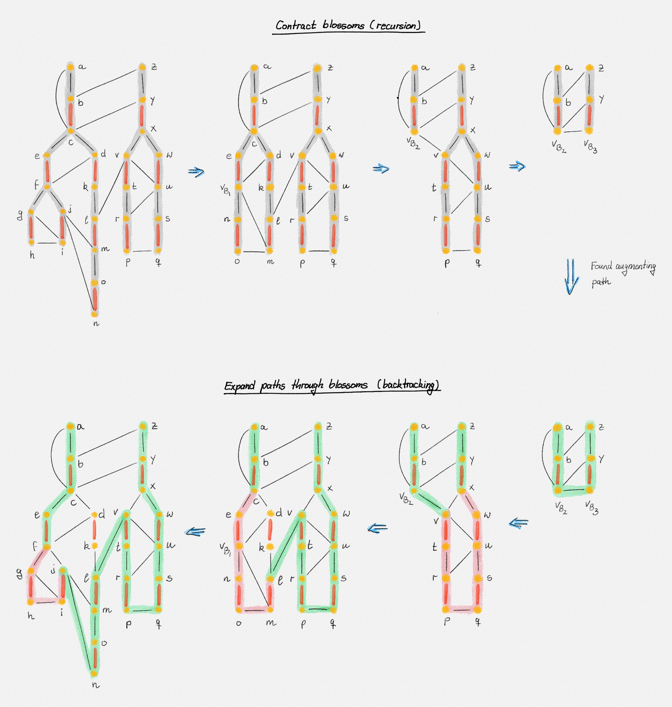
Figure 7.27: Illustration of the search for an augmenting path by Edmonds's algorithm. The top row shows, left to right, a sequence of graphs on which the algorithm recurses. The left graph is the input graph. Each subsequent graph is obtained from the previous one by contracting a blossom. The alternating forest is shown shaded. The bottom row shows how these blossoms are re-expanded after finding the augmenting path shown in the bottom-right figure. Each expansion maintains the augmenting path (green) by splitting it into the two subpath before and after \(v_{B_i}\) and then splicing these two pieces back together using an even alternating path inside the blossom (pink).

7.7.2. Gabow's Algorithm*

Coming soon!

8. Coping with NP-Hardness

Having discussed a range of advanced techniques to obtain polynomial-time algorithms for various graph problems beyond the scope of an introductory algorithms class, we leave the realm of problems that can be solved in polynomial time and focus on techniques for solving NP-hard problems now. We will focus almost exclusively on NP-hard optimization problems.

In this chapter, we use the vertex cover problem as an introductory example to highlight some of the central challenges and techniques for coping with NP-hardness. After this brief overview given in this chapter, the remaining chapters in these notes discuss a range of techniques that can be used to design approximation algorithms and techniques for designing fast exponential-time algorithms to solve NP-hard optimization problems.

8.1. The Vertex Cover Problem

Consider a computer network whose traffic we want to monitor in order to protect against attacks. We are required to observe every packet sent across any link in the network. An easy way to ensure this is to place a monitoring appliance on every network node. The appliance placed on a node now monitors the packets arriving at and leaving from this node. Clearly, this ensures that we observe every packet. However, these appliances are costly and intrusive. Thus, we would like to minimize the number of appliances we install. There is no need to place appliances on all nodes; it suffices to ensure that every link has at least one endpoint with an appliance on it. This idea is formalized as follows:

Given an undirected graph \(G = (V, E)\), a vertex cover of \(G\) is a subset of vertices \(C \subseteq V\) such that every edge in \(E\) has at least one endpoint in \(C\). See Figure 8.1.

Figure 8.1: Coming soon!

Vertex cover problem: Given a graph \(G = (V, E)\),find a vertex cover of minimum size or, if the vertices have weights, of minimum weight.

This is a classical NP-hard problem, so it cannot be solved exactly in polynomial time unless \(\textrm{P} = \textrm{NP}\).

8.2. Approximation Algorithms

Since we should not expect to solve any NP-hard optimization problem optimally in polynomial time, a natural question we may ask is whether we can obtain a suboptimal but good solution in polynomial time.

Heuristics are one way to try to find good solutions efficiently, and they can be extremely effective in practice. A downside of heuristics is that they do not provide any guarantees: They may produce very good solutions in practice, but we cannot prove that they always provide good solutions; or they may always produce very good solutions and do so quickly in practice, but we cannot prove that the algorithms are guaranteed to be fast.

We do not discuss heuristics further in these notes and instead focus on (polynomial-time) approximation algorithms. In contrast to heuristics, these are algorithms for which we can prove that they are fast, that they always run in polynomial time, and we are able to provide a provable bound on how much worse than an optimal solution the computed solution may be.

Let us formalize this notion of "bounding how bad the computed solution can be":

A \(\boldsymbol{c}\)-approximation algorithm for some minimization problem \(P\) with objective function \(f\) is an algorithm which, for any instance \(I\) of \(P\), computes a solution \(S\) whose objective function value \(f(S)\) is at most \(c \cdot \textrm{OPT}(I)\), where \(\textrm{OPT}(I)\) denotes the objective function value of an optimal solution of \(P\) on the input \(I\).

The factor \(c\) is called the approximation ratio achieved by the algorithm.

If \(P\) is a maximization problem, then a \(c\)-approximation algorithm for \(P\) computes a solution \(S\) for any instance \(I\) of \(P\) whose objective function value is \(f(S) \ge c \cdot \textrm{OPT}(I)\).

In the case of the vertex cover problem, this means that for any input graph \(G\), a \(c\)-approximation algorithm is guaranteed to compute a vertex cover that is at most \(c\) times bigger than a minimum vertex cover of \(G\).

Finding the Optimal Objective Function Value is the Hard Part

It is not hard to prove that the hard part of solving an NP-hard optimization problem \(P\) is finding \(\textrm{OPT}(I)\) for any instance \(I\) of \(P\): Assume we are given some polynomial-time algorithm \(\mathcal{A}\) which, given an instance \(I\) of \(P\) and some threshold \(t\), decides whether \(\textrm{OPT}(I) \le t\). This algorithm doesn't even compute \(\textrm{OPT}(I)\): It only decides whether \(\textrm{OPT}(I) \le t\). Given such an algorithm \(\mathcal{A}\), we can use it to design a polynomial-time algorithm that finds an optimal solution of \(P\) on the input \(I\). Since \(P\) is NP-hard, we believe that there is no polynomial-time algorithm that finds an optimal solution for any given instance of \(P\). Thus, a polynomial-time algorithm \(\mathcal{A}\) that decides whether \(\textrm{OPT}(I) \le t\) is also unlikely to exist.

This is a major problem for designing approximation algorithms: In order to prove a bound on the approximation ratio of a given algorithm, we need to compare the objective function value of the computed solution with the optimal objective function value, but computing the optimal objective function value is NP-hard. How do we bound the approximation ratio then? The answer is, we need to find a good lower bound (for minimization problems) or upper bound (for maximization problems) on \(\textrm{OPT}(I)\).

For the vertex cover problem, we need to establish a lower bound \(\ell\) on the size of any vertex cover of the input graph \(G\). In particular, \(\textrm{OPT}(G) \ge \ell\). If we can argue that our algorithm computes a vertex cover of size at most \(c\cdot\ell\), then this vertex cover also has size at most \(c\cdot\textrm{OPT}(G)\), that is, the algorithm is a \(c\)-approximation algorithm.

What is a good lower bound on the size of any vertex cover of some graph \(G\)? Consider a maximal matching \(M\) of \(G\). See Figure 8.2. Since no two edges in \(M\) share an endpoint, no vertex of \(G\) covers more than one edge in \(M\), that is, we need at least \(|M|\) vertices to cover the edges in \(M\). Thus, any vertex cover of \(G\) has size at least \(|M|\).

Figure 8.2: Coming soon!

Now consider the set \(C_M = \{ u, v \mid (u,v) \in M \}\). Clearly, \(|C_M| = 2|M|\). Moreover, it is a vertex cover of \(G\). Indeed, if there exists an edge \((u,v)\) not covered by \(C_M\), then \(u,v \notin C_M\), that is, the edge \((u,v)\) does not share any endpoint with any edge in \(M\). Thus, \(M \cup \{(u,v)\}\) is a matching, a contradiction because \(M\) is a maximal matching.

This gives a simple linear-time \(2\)-approximation algorithm for the vertex cover problem: Compute a maximal matching of \(G\) and return the set of all matched vertices.

Theorem 8.1: There exists a linear-time \(2\)-approximation algorithm for the vertex cover problem.

Inapproximability and Families of Tight Inputs

Given any algorithm, we should always ask ourselves whether it can be improved. In the case of approximation algorithms, the central question is whether the approximation guarantee can be improved. This question has to be asked carefully, in order to obtain a meaningful answer. For example, the answer is always yes if we place no bound on the running time of the better algorithm we hope to obtain: If the optimal is computable, we can always obtain an optimal solution given enough time. The right way to ask this question is whether there exists a polynomial-time algorithm that provides a better approximation guarantee. If the problem is NP-hard, no polynomial-time algorithm that solves the problem exactly exists unless \(\textrm{P}=\textrm{NP}\).

For some problems, we are able to prove that they cannot be approximated below a certain threshold unless \(\textrm{P}=\textrm{NP}\). For example, we will show that, assuming that \(\textrm{P} \ne \textrm{NP}\), \(2\) is essentially the best approximation guarantee for the \(k\)-center problem that can be obtained in polynomial time. The way to prove this is to show that an algorithm with approximation ratio \(c\) sufficiently smaller than \(2\) can be used to solve some NP-hard decision problem. Since the latter is not possible in polynomial time unless \(\textrm{P} = \textrm{NP}\), no polynomial-time algorithm with approximation factor \(c\) exists, again unless \(\textrm{P} = \textrm{NP}\).

For other problems, we are able to prove that they can be approximated arbitrarily well. The bin packing problem and the travelling salesman problem are two such problems. They can be approximated, in polynomial time, to within a factor of \(1 + \epsilon\) of an optimal solution, for any constant \(\epsilon > 0\). Such a solution is called a polynomial-time approximation scheme (PTAS). There is, however, a price that needs to be paid for improved approximation guarantees: The running time of the algorithm increases as \(\epsilon\) decreases. This should not be surprising because, as \(\epsilon\) approaches \(0\), the running time should approach exponential time, given that we are trying to solve an NP-hard optimization problem. Since the running time of the algorithm depends on \(\epsilon\), we should ask how bad the dependence of the running time on \(\epsilon\) is. If the dependence is polynomial in \(\frac{1}{\epsilon}\), we call the PTAS a fully polynomial-time approximation scheme (FPTAS). A PTAS that is not an FPTAS can have an exponential or worse dependence on \(\frac{1}{\epsilon}\); it only has to be possible to compute a \((1 + \epsilon)\)-approximation in polynomial time for any fixed \(\epsilon > 0\).

Both inapproximability results, such as the inapproximability result for the \(k\)-center problem mentioned above, and (F)PTASs require some care to obtain. A more immediate question we can ask about a given approximation algorithm, which is usually much easier to answer, is whether its analysis can be improved. Thus, we are not asking whether there is a better algorithm, only whether we could possibly prove that the algorithm we have already developed does in fact achieve a better approximation ratio than we have proven so far. Since every approximation algorithm is based on some lower or upper bound on the optimal objective function value \(\textrm{OPT}\), the approximation ratio the algorithm is able to guarantee depends on the quality of this lower or upper bound. Thus, we may ask whether there exists a family of tight inputs, an infinite family of inputs for which the algorithm cannot perform significantly better than the bound we proved.¹

As an example, consider the matching-based approximation algorithm for the vertex cover problem. A family of tight inputs is provided by the set of complete bipartite graphs \(K_{n,n}\) on \(2n\) vertices. See Figure 8.3.

Figure 8.3: Coming soon!

Any maximal matching of \(K_{n,n}\) includes \(n\) edges and thus matches all \(2n\) vertices of the graph. The approximation algorithm thus includes all \(2n\) vertices in the vertex cover. However, a vertex cover of size \(n\) exists: the \(n\) vertices in one of the two bipartitions cover all edges. Thus, the vertex cover the algorithm computes for \(K_{n,n}\) is by a factor \(2\) larger than an optimal vertex cover; there exist an infinite number of inputs for which the algorithm does not achieve an approximation guarantee better than \(2\).

Summary

To summarize, the first approach to solving NP-hard optimization problems we consider is to compute good approximations of optimal solutions in polynomial time.

• The proof that these algorithms output a \(c\)-approximation of an optimal solution for every possible input and some fixed factor \(c\) requires us to come up with a lower bound or upper bound on the objective function value of an optimal solution to which we can compare the solution computed by the algorithm. We cannot compute the optimal objective function value, as this is the hard core of the problem.

• We may ask whether the approximation ratio achieved by an algorithm is the best possible. Such a result is called an inapproximability result, a proof that there is no polynomial-time algorithm that achieves an approximation ratio better than a certain threshold unless \(\textrm{P} = \textrm{NP}\).

• The simpler question is whether our analysis of a given algorithm is tight, whether we can prove that there are inputs where the solution output by the algorithm is exactly as bad as predicted by our analysis.

• Finally, there are problems that can be approximated arbitrarily well, to within an approximation ratio of \(1 + \epsilon\) for an arbitrary constant \(\epsilon > 0\). Such algorithms are called polynomial-time approximation schemes. We will not discuss these in detail in this course, even though they are often based on really beautiful ideas. You may for example have a look at the PTAS for the metric travelling salesman problem by Sanjeev Arora. One excuse for not covering PTASs in this course, apart from having only limited time and having to choose judiciously which problems and techniques to cover, is that in spite of their beauty, PTASs are often impractical. They often use fairly complex algorithmic building blocks and, once we choose very small values of \(\epsilon\) to benefit from the PTAS's ability to provide very tight approximations of optimal solutions, they are often slower in practice than carefully implemented exponential-time algorithms for the same problem, which actually produce optimal solutions.

8.3. Exponential-Time Algorithms

What if we do not want to settle for an approximation and instead insist on finding an optimal solution? In the case of the vertex cover problem, we want to find a vertex cover of minimum size. Given that the vertex cover problem is NP-hard, we should not hope to be able to find an optimal vertex cover in polynomial time unless \(\textrm{P} = \textrm{NP}\), that is, we have to accept that any exact algorithm for the vertex cover problem takes exponential time in the worst case. This gives rise to two natural questions:

The first question is analogous to the central question in designing classical polynomial-time algorithms: What is the fastest exponential-time algorithm we can design for a given NP-hard problem? For sorting, for example, an \(O(n \lg n)\)-time algorithm such as Merge Sort is preferable to an \(O\bigl(n^2\bigr)\)-time algorithm such as Insertion Sort, except for very small inputs. The gap between these two running times is a factor of \(\Theta\bigl(\frac{n}{\lg n}\bigr)\), which is rightly considered a significant improvement. However, this type of improvement pales in comparison to the types of improvements we can achieve for NP-hard problems by carefully designing exponential-time algorithms for these problem.

As an introductory example, we discuss three algorithms for the vertex cover problem below, two with running time \(O^*\bigl(2^n\bigr)\) and the other with running time \(O^*\bigl(1.619^n\bigr)\). When discussing exponential-time algorithms, we almost always write \(O^*(f(n))\) to denote running times of the form \(O(f(n) \cdot n^c)\), where \(f(n)\) is an exponential function. In other words, the \(O^*\)-notation ignores polynomial factors in the running time, which is justified because these polynomial factors are negligible in comparison to the exponential portion \(f(n)\) of the running time. How much of an improvement is a decrease of the algorithm's running time from \(O^*\bigl(2^n\bigr)\) to \(O^*\bigl(1.619^n\bigr)\)? Well, the gap is \(\bigl(\frac{2}{1.619}\bigr)^n \ge 1.235^n\), which dwarves the \(\Theta\bigl(\frac{n}{\lg n}\bigr)\) improvement achieved by Merge Sort in comparison to Insertion Sort. The point is that even seemingly small improvements in the base of the running time of exponential-time algorithms has a much greater impact on the running time of the algorithm than much more impressive-looking improvements in the running times of polynomial-time algorithms. Thus, it is worthwhile to look for the fastest possible exponential-time algorithms we can find for NP-hard problems.

The second question we ask about exponential-time algorithms is whether we can decouple the exponential explosion of their running times from the input size and instead make it depend only on some hardness parameter \(k\). We consider this question in the next section.

A Naïve Vertex Cover Algorithm and Exponential Branching

How quickly can we solve the vertex cover problem naïvely? Since a vertex cover is a subset of the vertices of \(G\), we can enumerate all \(2^n\) subsets of \(V\) and, for each, test whether it is a vertex cover, which takes \(O(m)\) time, constant time per edge. Thus, a naïve algorithm for the vertex cover problem takes \(O\bigl(2^n m\bigr) = O^*\bigl(2^n\bigr)\) time. Can we do better? As it turns out, we can. As a basis for this improvement, we first discuss one important technique for solving NP-hard problems efficiently: branching. We study this technique in greater detail in Chapter 16.

Consider an arbitrary edge \(e = (u,v)\). Any vertex cover has to contain at least one of its endpoints. If we include \(u\) in a vertex cover \(C\), then \(C \setminus {u}\) must be an optimal vertex cover for the subgraph \(G - u = G[V \setminus \{u\}]\)¹ because any vertex cover \(C'\) of \(G - u\) can be extended to a vertex cover \(C' \cup \{u\}\) of \(G\). Similarly, if we include \(v\) in a vertex cover \(C\), then \(C \setminus \{v\}\) must be an optimal vertex cover for the subgraph \(G - v\). Thus, we obtain the following simple recursive algorithm for finding a minimum vertex cover of a graph \(G = (V, E)\):

• If \(E = \emptyset\), then \(\emptyset\) is a vertex cover of \(G\) and no smaller vertex cover exists, so we return this vertex cover.
• If \(E \ne \emptyset\), then pick an arbitrary edge \((u,v) \in E\) and compute two optimal vertex covers \(C_u\) of \(G - u\) and \(C_v\) of \(G - v\). Return the smaller of \(C_u \cup \{u\}\) and \(C_v \cup \{v\}\).

We call this algorithm a branching algorithm because it "branches" on the possible choices of which endpoint of the edge \((u,v)\) to include in the vertex cover. For each choice, we end up with a different subproblem, which we solve by invoking the algorithm recursively.

Each recursive call is easily implemented in \(O(n)\) time. The two graphs \(G - u\) and \(G - v\) each have one less vertex than \(G\). Thus, the running time of this algorithm is given by the recurrence \(T(n) = O(n) + 2T(n-1)\), which is easily seen to have the solution \(T(n) = O\bigl(2^n n\bigr) = O^*\bigl(2^n\bigr)\).

Theorem 8.2: The vertex cover problem can be solved in \(O^*\bigl(2^n\bigr)\) time.

Improved Branching Rules

A common approach to designing fast exponential-time algorithms is to start with a simple and natural branching algorithm and then exploit insights into the structure of the problem to obtain better branching rules that lead to a lower fan-out or to a faster reduction of the input size in each branching step. The fan-out refers to the number of recursive calls that each invocation of the algorithm makes. The reduction of the input size refers to the sizes of the inputs of the recursive calls each invocation makes, relative to the input size of the current invocation. The simple branching algorithm for the vertex cover problem just discussed has fan-out \(2\), and the input of each recursive call has one vertex less than the input to the current invocation.

For the vertex cover problem, observe that there is some overlap between the two recursive calls in the branching algorithm in the previous section. The first vertex cover \(C_u \cup \{u\}\) we find is the smallest vertex cover that includes \(u\). The second vertex cover \(C_v \cup \{v\}\) is the smallest vertex cover that includes \(v\). However, the optimal vertex cover may include both \(u\) and \(v\). If this is the case, both recursive calls find the same vertex cover, at least potentially. This is redundant!

The problem is that the branching strategy was based on deciding which of the two endpoints of an edge to include in the vertex cover. A better strategy branches on the vertices, not edges, and decides for each vertex \(v\) whether to include it in the vertex cover or not. Again, if there are no edges, then the empty set is an optimal vertex cover. Thus, we can assume that the edge set is non-empty. We pick a vertex \(v\) of maximum degree. This vertex has degree at least \(1\). If \(v\) is in an optimal vertex cover \(C\), then \(C \setminus \{v\}\) is an optimal vertex cover of \(G - v\), just as in the edge-branching algorithm. If \(v\) is not in the vertex cover, then all of its neighbours must be in the vertex cover because all edges incident to \(v\) must be covered and we do not use \(v\) to cover them. Since the set of neighbours of \(v\), \(N(v)\), covers all edges incident to the vertices in \(N[v] = \{v\} \cup N(v)\), \(C \setminus N(v)\) must be an optimal vertex cover of the graph \(G - N[v] = G[V \setminus N[v]]\). We often refer to \(N(v)\) as the open neighbourhood of \(v\) and to \(N[v]\) as the closed neighbourhood of \(v\). This gives the following improved algorithm:

• If \(E = \emptyset\), return \(\emptyset\) as an optimal vertex cover of \(G\).
• If \(E \ne \emptyset\), then let \(v\) be a vertex of maximum degree. Recursively compute a vertex covers \(C_v\) of \(G - v\) and a vertex cover \(C_{N(v)}\) of \(G - N[v]\) and return the smaller of \(C_v \cup \{v\}\) and \(C_{N(v)} \cup N(v)\).

As before, \(G - v\) has \(n-1\) vertices. Since \(v\) has degree at least \(1\), we have \(|N[v]| \ge 2\), that is, \(G - N[v]\) has at most \(n-2\) vertices. Thus, the running time of this algorithm is given by the recurrence \(T(n) \le O(n) + T(n-1) + T(n-2)\), which has the solution \(T(n) = O^*\Bigl(\Bigl(\frac{1 + \sqrt{5}}{2}\Bigr)^n\Bigr) = O^*\bigl(1.619^n\bigr)\).

Theorem 8.3: The vertex cover problem can be solved in \(O^*\bigl(1.619^n\bigr)\) time.

Further careful improvements and better analysis techniques, discussed in Chapters 16 and 17, reduce this running time further.

8.4. Fixed-Parameter Tractability

Let us return to the question already touched upon in the previous section: Can we decouple the exponential running time of an algorithm that solves an NP-hard optimization problem exactly from the input size and instead limit the exponential explosion to some hardness parameter?

The first question we need to answer is what makes a good parameter? There are many possible answers to this question. From a purely theoretical point of view, it may be interesting to understand which structural properties of an input make a problem hard or easy on this input. For example, the treewidth of a graph captures how tree-like a graph is. It turns out that a very large number of NP-hard graph problems can be solved in \(O(f(k) n)\) time, where \(k\) is the treewidth of the given graph. Thus, if \(k\) is small, if the graph is very tree-like, we can solve these problems in linear time, in spite of their NP-hardness.

These results are theoretically interesting and the techniques necessary to prove them are clever. From a practical point of view, however, these algorithms are often unsatisfactory. What reason do we have to believe that real-world graphs have small treewidth, that is, are very tree-like? More natural parameter choices are often driven by the problem we want to solve. Throughout these notes, we choose the objective function value as the parameter. For the vertex cover problem, we thus want to find an algorithm with running time \(O^*(f(k))\), where \(k\) is the size of the computed vertex cover. We can argue that this is a natural parameter because, if the vertex cover is not small, we probably do not care about an exact solution anyway.

So how do we design an algorithm with running time \(O^*(f(k))\) for the vertex cover problem. The first observation, which applies to all NP-hard problems, is that we can focus on the decision version of the problem: Given a pair \((G,k)\), where \(G\) is an undirected graph and \(k\) is an integer, we only want to decide whether \(G\) has a vertex cover of size at most \(k\). Such a decision algorithm is easily augmented to also return a vertex cover of size at most \(k\) if such a vertex cover exists. Given such a decision algorithm, say with running time \(O^*\bigl(c^k\bigr)\) for some constant \(c\), we can compute an optimal vertex cover by first trying to find a vertex cover of size \(0\), then of size \(1\), then of size \(2\), and so on until we finally obtain an affirmative answer. If \(k\) is the size of the computed vertex cover, this linear guessing approach takes \(\sum_{i=0}^k O^*\bigl(c^i\bigr) = O^*\bigl(c^k\bigr)\) time, that is, the final iteration dominates the running time of the whole algorithm. What is left is to design an algorithm that takes \(O^*\bigl(c^k\bigr)\) time to decide whether a given graph has a vertex cover of size at most \(k\). Again, we use branching to do this:

• If \(k < 0\), we answer "No". There clearly does not exist a vertex cover of negative size. So assume from here on that \(k \ge 0\).

• If \(E = \emptyset\), we answer "Yes" (and return the empty set) because the empty set is a valid vertex cover and has size \(0 \le k\).

• Otherwise, we once again choose a vertex \(v\) of maximum degree. We make two recursive calls to decide whether \(G - v\) has a vertex cover of size at most \(k-1\) and whether \(G - N[v]\) has a vertex cover of size at most \(k - |N(v)|\).

  If the first recursive call answers "Yes" (and returns a vertex cover \(C_v\) of \(G - v\) of size at most \(k - 1\)), then we answer "Yes" and return \(C_v \cup \{v\}\), which is a vertex cover of \(G\) of size at most \(k\).

  If the second recursive call answers "Yes" (and returns a vertex cover \(C_{N(v)}\) of \(G - N[v]\) of size at most \(k - |N(v)|\)), then we answer "Yes" and return \(C_{N(v)} \cup N(v)\), which is a vertex cover of \(G\) of size at most \(k\).

  If both recursive calls answer "No", then we answer "No". This is correct because any vertex cover \(C\) of \(G\) includes \(v\) or all vertices in \(N(v)\). If \(|C| \le k\) and \(v \in C\), then \(C \setminus \{v\}\) is a vertex cover of \(G - v\) of size at most \(k-1\), that is, the first recursive call returns "Yes". If \(|C| \le k\) and \(v \notin C\), then \(N(v) \subseteq C\) and \(C \setminus N(v)\) is a vertex cover of \(G - N[v]\) of size at most \(k - N(v)\), that is, the second retursive call returns "Yes". Thus, if both recursive calls return "No", then \(G\) has no vertex cover of size at most \(k\).

The key observation now is that the parameter of both recursive calls is at most \(k-1\) because \(|N(v)| \ge 1\). Thus, the running time of this algorithm is given by the recurrence \(T(n,k) = O(n) + 2T(n,k-1)\), which has the solution \(T(n,k) = O^*\bigl(2^k\bigr)\).

Theorem 8.4: The vertex cover problem can be solved in \(O^*\bigl(2^k\bigr)\) time.

If you paid attention, you should have an obvious question: We used the same branching strategy as in the improved exponential time algorithm, but we only obtained a bound of \(O^*\bigl(2^k\bigr)\) on the running time of the parameterized algorithm while the running time of the exponential-time algorithm was \(O^*\bigl(1.619^n\bigr)\). Why is that?

The reason is that the size of the input to the second recursive call is at most \(n - 2\) because both \(v\) and the vertices in \(N(v)\) are removed from the input to this recursive call. The parameter, on the other hand, may be reduced by only \(1\) because in the second branch, only the vertices in \(N(v)\) but not \(v\) are included in the vertex cover. To obtain better parameterized algorithms for the vertex cover problem, we need more advanced branching rules, which we discuss in Chapter 16.

So what does the term "fixed-parameter tractability" refer to? Intuitively, it captures the idea that if we consider only inputs for which the hardness parameter is bounded by a constant, then we can solve the problem on such inputs in polynomial-time: the problem becomes "tractable" on such inputs. Technically, an algorithm with running time \(O\bigl(n^{f(k)}\bigr)\) also satisfies this condition: If \(k\) is a constant, then the running time of the algorithm is polynomial. To consider a problem fixed-parameter tractable, however, we impose a stricter requirement:

The input to any parameterized algorithm for some problem \(P\) consists of a pair \((I, k)\), where \(I\) is an instance of \(P\) and \(k\) is an upper bound on the hardness parameter of \(I\).

A problem \(P\) parameterized by some parameter \(k\) is fixed-parameter tractable if there exists an algorithm that solves \(P\) on any parameterized instance \((I, k)\) in \(O(f(k) \cdot n^c)\) time.

In other words, we allow the running time of the algorithm to have an exponential or worse dependence on the parameter \(k\), as expressed by the function \(f(k)\), but the running time of the algorithm must depend only polynomially on the input size. More importantly, these two factors of the running time must be independent of each other: The polynomial dependence of the running time of the algorithm must be independent of the parameter.

The motivation for this restrictive definition of fixed-parameter tractability is that algorithms with running time \(O\bigl(n^{f(k)}\bigr)\) are efficient only for very small values of \(k\).

9. Greedy Approximation Algorithms and Layering

In CSCI 3110, you should have received a first introduction to greedy algorithms. The main characteristic of a greedy algorithm is that it makes "local" choices: It constructs a solution one choice at a time, and it makes each choice based on what seems best at the moment, without consideration for how this choice affects future choices. For example, Kruskal's algorithm builds a minimum spanning tree by repeatedly picking the cheapest edge that can still be added to the current partial spanning tree without creating a cycle. We were able to prove that once we obtain a tree, the result must be a minimum spanning tree.

The problems discussed in CSCI 3110 had the remarkable property that it was possible to arrive at a globally optimal solution by making such local choices. For many problems, this is not the case: We may be able to obtain a good solution by making local choices, but the solution may not be optimal. Sometimes, making greedy choices may lead to arbitrarily bad solutions. For other problems, greedy choices may be the basis for very good heuristics in practice. While heuristics may work very well in practice, they have the disadvantage that they usually do not provide any provable guarantees on how much worse the computed solution is than an optimal solution. In this chapter, we consider a number of problems for which we can prove that a greedy algorithm computes a \(c\)-approximation of an optimal solution, for some small factor \(c\).

• As a warm-up exercise, we start with the bin packing problem in Section 9.1. We prove that a very simple greedy algorithm produces a \(2\)-approximation of an optimal solution.

• The set cover problem is a generalization of the vertex cover problem, which I introduced in Chapter 8. We discuss two algorithms for the set cover problem. A fairly natural greedy algorithm computes an \(O(\lg n)\)-approximation of an optimal set cover. We discuss this algorithm in Section 9.2. A second algorithm, discussed in Section 9.3, computes an \(f\)-approximation, where \(f\) is the maximum number of sets in the input that any element occurs in. This algorithm is based on an interesting technique, called layering. The main idea of layering is to slice (layer) the input into subproblems such that a good approximation of an optimal solution can be obtained easily on each layer. By combining the solutions on the different layers, we then obtain a good approximation for the entire input. It turns out that every approximation algorithm for the set cover problem achieves one of these two approximation ratios: \(f\) or \(O(\lg n)\).

• We conclude the chapter by discussing, in Section 9.4, the feedback vertex set problem, which is a second problem for which layering produces a good approximate solution.

9.1. Bin Packing

In the bin packing problem, we are given a collection of \(n\) items of sizes \(s_1, \ldots, s_n\). Each size \(s_i\) satisfies \(0 < s_i \le 1\). Our goal is to pack these items into as few bins of size \(1\) as possible. In other words, we want to partition the set \(S = \{s_1, \ldots, s_n\}\) into as few subsets \(B_1, \ldots, B_k\) as possible so that \(\sum_{s \in B_j} s \le 1\) for all \(1 \le j \le k\). From here on, we will not distinguish between an item and its size.

As example, we could have five items of size \(0.6\), \(0.3\), \(0.4\), \(0.7\), and \(1\). They require \(3\) bins to be packed if we pack the first and third item into a bin, the second and fourth item into a bin, and the fifth item into a bin. This fills every bin fully but does not overpack any bin because \(0.6 + 0.4 = 1\) and \(0.3 + 0.7 = 1\).

Figure 9.1: Coming soon!

9.1.1. A Simple Greedy Algorithm

The following is probably the most natural greedy algorithm one can think of: Start by packing the first item \(s_1\) into a new bin \(B_1\). For every subsequent item \(s_i\), we check whether there exists a bin \(B_j\) such that \(\sum_{s \in B_j} s \le 1 - s_i\). If so, we choose an arbitrary such bin \(B_j\) and add \(s_i\) to \(B_j\). Otherwise, we create a new bin \(B_{k+1}\) (where \(k\) is the number of bins created so far) and add \(s_i\) to this new bin. Let us call this algorithm First Fit because it adds \(s_i\) to the first bin where it fits.

If we apply First Fit to the five items in the example in Figure 9.1, we use \(4\) bins, one more than the optimal number. First Fit places the first item into its own bin and then places the second item into the same bin because it fits. This fills the first bin to \(0.6 + 0.3 = 0.9\). Each of the remaining three items then needs to be packed into its own bin.

Figure 9.2: Coming soon!

In this example, the solution computed by First Fit is not optimal, but it is less than a factor \(2\) away from an optimal solution: The solution computed by First Fit uses \(4\) bins. The optimal solution uses \(3\) bins. Let us prove that this is true for every possible input:

Theorem 9.1: The First Fit algorithm computes a \(2\)-approximation for the bin packing problem.

Proof: As discussed in Section 8.2, the key to bounding the approximation ratio of the algorithm is to provide the right lower bound on the number of bins in an optimal solution. Here, a very simple lower bound is enough: The total size of the bins cannot be less than the total size of all items. Thus, since every bin has size \(1\), the optimal number of bins is \(\textrm{OPT} \ge \sum_{i=1}^n s_i\). We prove that First Fit uses at most \(2\sum_{i=1}^n s_i \le 2 \cdot \textrm{OPT}\) bins.

We group the bins into pairs. If the number of bins is odd, then the last bin is ignored in this grouping. Each pair of bins \((B_i, B_j)\) satisfies \(\sum_{s \in B_i \cup B_j} > 1\). Indeed, assume that \(i < j\) and let \(s_h\) be the first element in \(B_j\). If \(\sum_{s \in B_i \cup B_j} s \le 1\), then \(\sum_{s \in B_i} \le 1 - s_h\). Since this is true at the end of the algorithm, it is also true when the algorithm decides into which bin to place \(s_h\). On the other hand, since \(s_h\) is the first item we place into bin \(B_j\), \(s_h\) does not fit into any of the bins \(B_1, \ldots, B_{j-1}\) at the time we place \(s_h\) into bin \(B_j\). Since \(i < j\), this is a contradiction.

Since every pair of bins \((B_i, B_j)\) satisfies \(\sum_{s \in B_i \cup B_j} s > 1\). we have \(\sum_{i=1}^n s_i > p\), where \(p\) is the number of pairs of bins. Since \(\textrm{OPT} \ge \sum_{i=1}^n s_i\), this implies that \(\textrm{OPT} > p\), that is, \(\textrm{OPT} \ge p + 1\). The number of bins we use is at most \(2p + 1 < 2p + 2 \le 2 \cdot \textrm{OPT}\), that is, First Fit computes a \(2\)-approximation of the optimal number of bins. ▨

9.1.2. A Family of Tight Inputs

Recall that once we have an approximation algorithm for an NP-hard optimization problem, we should ask the question whether the approximation ratio achieved by our algorithm is the best possible. We will do this for some problems in these notes, but not for all of them. Also recall that this question comes in two flavours. The harder question is whether there exists any algorithm that achieves a better approximation ratio than our algorithm. The easier question is whether the analysis of our algorithm is tight, whether it does in fact achieve a better approximation ratio than we were able to prove.

For the bin packing problem, we consider the second question. It turns out that our analysis is not tight. It has been shown fairly recently that First Fit achieves an approximation ratio of \(1.7\) and that this analysis is in fact tight, that is, that there exists an infinite family of inputs for which First Fit does indeed produce a solution that is \(1.7\) times worse than an optimal solution. This analysis of First Fit requires some care though. Here, we will be content with proving that there exists an infinite family of inputs for which First Fit computes a solution that is \(\frac{5}{3} \approx 1.667\) times worse than an optimal solution.

Consider an input consisting of \(18n\) items, shown in Figure 9.3. The first \(6n\) items have size \(0.15\), the next \(6n\) items have size \(0.34\), and the final \(6n\) items have size \(0.51\). One item of size \(0.15\), one item of size \(0.34\), and one item of size \(0.51\) fit in a bin, since their combined size is exactly \(1\). Thus, \(\textrm{OPT} = 6n\). First Fit packs the first \(6n\) items into \(n\) bins, packing \(6\) items into each bin. This uses \(0.9\) space in each of these \(n\) bins, that is none of these bins can accommodate any further items. The next \(6n\) items are packed into \(3n\) bins, \(2\) items per bin. This uses \(0.68\) space in each of these \(3n\) bins, that is none of these bins can accommodate any of the remaining items of size \(0.51\). Thus, the final \(6n\) items are packed into one bin each, using \(6n\) bins in total. Therefore, First Fit uses \(10n\) bins in total. This is a \(\frac{5}{3}\)-approximation of the optimal number of bins, which is \(6n\).

Figure 9.3: Coming soon!

9.2. Greedy Set Cover

The set cover problem is an extension of the vertex cover problem:

Given a universe \(U\) and a collection \(\mathcal{S}\) of subsets of \(U\) such that \(\bigcup_{S \in \mathcal{S}} = U\), a set cover is a subset \(\mathcal{C} \subseteq \mathcal{S}\) such that \(\bigcup_{S \in \mathcal{C}} = U\). In other word, \(\mathcal{C}\) contains at least one set from \(\mathcal{S}\) that includes each element of \(U\).

Unweighted Set Cover Problem: Given a universe \(U\) and a collection \(\mathcal{S}\) of subsets of \(U\) such that \(\bigcup_{S \in \mathcal{S}} = U\), find a set cover \(\mathcal{C} \subseteq \mathcal{S}\) of \(U\) of minimum size.

Weighted Set Cover Problem: Given a universe \(U\), a collection \(\mathcal{S}\) of subsets of \(U\) such that \(\bigcup_{S \in \mathcal{S}} = U\), and a weight function \(w : \mathcal{S} \rightarrow \mathbb{R}^+\), find a set cover \(\mathcal{C} \subseteq \mathcal{S}\) of \(U\) of minimum weight \(w(\mathcal{C}) = \sum_{S \in \mathcal{C}}w_S\).

As an example, consider a universe \(U = \{a,b,c,d,e\}\) and four subsets \(S_1 = \{a,b,c\}\), \(S_2 = \{b,d,e\}\), \(S_3 = \{a,b\}\), and \(S_4 = \{a,c\}\). The collection \(\mathcal{C} = \{S_1, S_2\}\) is a set cover because \(S_1 \mathcal{c}up S_2 = U\). It is a set cover of minimum size because we clearly cannot cover \(U\) with only a single set in \(\mathcal{S} = \{S_1, S_2, S_3, S_4\}\). Given a weight function defined as \(w_{S_1} = 3\), \(w_{S_2} = 4\), \(w_{S_3} = 1\), and \(w_{S_4} = 1\), however, it is not a minimum-weight set cover. Its weight is \(w(\mathcal{C}) = w_{S_1} + w_{S_2} = 7\), whereas the set \(\mathcal{C}' = \{S_2, S_3, S_4\}\) also covers \(U\) but has weight \(w(\mathcal{C}') = w_{S_2} + w_{S_3} + w_{S_4} = 6\).

Figure 9.4: Coming soon!

Clearly, any algorithm that can solve the weighted set cover problem can also solve the unweighted set cover problem because the unweighted set cover problem is a special case of the weighted set cover problem where every set has weight \(1\). By the following exercise, the restriction of the weight function in the weighted set cover problem to positive weights is not a serious one:

Exercise 9.1: Assume you are given an algorithm \(\mathcal{A}\) that computes a \(c\)-approximation of an optimal weighted set cover under the assumption that all sets have strictly positive weights. If \(c = 1\), then \(\mathcal{A}\) computes an optimal weighted set cover. Prove that you can use \(\mathcal{A}\) to also compute a \(c\)-approximation of an optimal weighted set cover when the sets have arbitrary weights.

In this section, we discuss a greedy algorithm that computes an \(O(\lg n)\)-approximation of an optimal weighted set cover.

9.2.1. The Right Greedy Choice

So what is a good greedy choice for the set cover problem? Two natural choices come to mind:

• Pick the cheapest set (set of minimum weight) in each iteration or
• Pick the set that covers the most elements.

Clearly, picking cheap sets seems to be a good strategy because our goal is to minimize the total weight of the sets in the set cover. This strategy fails when there is a more expensive set that covers many elements. For example, consider the universe \(U = \{1, \ldots, n\}\) and a collection of sets \(\mathcal{S} = \{S_1, \ldots, S_{n+1}\}\), where \(S_i = \{i\}\) for \(1 \le i \le n\), and \(S_{n+1} = U\). The sets \(S_1, \ldots, S_n\) have weight \(1\) each, while the set \(S_{n+1}\) has weight \(2\). If we pick the cheapest set in each iteration, we end up with the set cover \(\mathcal{C} = \{S_1, \ldots, S_n\}\). This set cover has weight \(n\). The optimal set cover consists of the single set \(S_{n+1}\) and has weight \(2\). Thus, we obtain only a \(\frac{n}{2}\)-approximation using the strategy of always picking the cheapest set in this example.

Figure 9.5: Coming soon!

The reason why always picking the cheapest set isn't a good strategy in this example is that \(S_{n+1}\) is only slightly more expensive than the other sets but covers many more elements, all elements in fact. This is the motivation for the second strategy. We hope that by always picking the set that covers the most elements, we include only few sets in the set cover. Thus, if the weights of the sets do not differ too much, this should be a reasonable strategy to minimize the weight of the computed set cover. We can defeat this strategy using the same example that we used to defeat the strategy of always picking the cheapest set, only this time we assign a very large weight to \(S_{n+1}\), say \(w_{S_{n+1}} = n^2\). In this case, picking the largest set produces a set cover of weight \(n^2\) whereas the set cover consisting of the sets \(S_1, \ldots, S_n\) has weight only \(n\).

Figure 9.6: Coming soon!

Picking large sets seemed to be a good strategy when these large sets are cheap. Otherwise, picking the cheapest sets works better. It seems that we need a strategy that takes both the size of the sets and their weights into account. What we really want is to cover all elements in \(U\) at a low cost per element. In the above example, when \(w_{S_{n+1}} = 2\), \(S_{n+1}\) covers all \(n\) elements at a cost of \(2\). The cost per element is thus only \(\frac{2}{n}\), whereas each set \(S_i\) with \(1 \le i \le n\) covers a single element \(i\) at cost \(1\) per element. In an amortized sense, \(S_{n+1}\) is the cheaper set. When \(w_{S_{n+1}} = n^2\), \(S_{n+1}\) covers the elements in \(U\) at a cost of \(n\) per element. This is much greater than the cost of covering each element \(i\) using its corresponding set \(S_i\). Thus, the set cover \(\{S_1, \ldots, S_n\}\) is the better choice in this case.

So let's try another strategy:

• Pick the set \(S_i\) that has minimum weight per element it covers, that is, pick the set \(S_i\) that minimizes the ratio \(\frac{w_{S_i}}{|S_i|}\).

This strategy certainly achieves the goal of taking both the weights of the chosen sets and their sizes into account, striking a balance between choosing cheap sets and large sets. It's still not quite the right strategy though: Consider the universe \(U = \{1, \ldots, 2n\}\) and sets \(S_1, \ldots, S_{n+2}\), where \(S_i = \{i, n+1, \ldots, 2n\}\) for all \(1 \le i \le n\), \(S_{n+1} = \{1, \ldots, n\}\), and \(S_{n+2} = \{n+1, \ldots, 2n\}\). Each of the sets \(S_1, \ldots, S_{n+1}\) has weight \(2\). The set \(S_{n+2}\) has weight \(1\). The set \(S_{n+2}\) has minimum weight per element, \(\frac{1}{n}\), so we choose this set first. Each of the sets \(S_1, \ldots, S_n\) has weight \(\frac{2}{n+1}\) per element, whereas the set \(S_{n+1}\) has weight \(\frac{2}{n}\) per element. Thus, after picking \(S_{n+2}\), we pick all of the sets \(S_1, \ldots, S_n\), which results in a set cover of weight \(2n + 1\). The optimal set cover is \(\{S_{n+1}, S_{n+2}\}\), which has weight \(3\). So what went wrong? Picking \(S_{n+2}\) is certainly a reasonable choice. After picking \(S_{n+2}\), however, picking \(S_{n+1}\) is a much better choice than picking any of the sets \(S_1, \ldots, S_n\): \(S_{n+1}\) contains \(n\) elements not already covered by \(S_{n+2}\), and it covers these elements at a cost of \(\frac{2}{n}\) per element. Each of the sets \(S_1, \ldots, S_n\) contains \(n + 1\) elements, but \(n\) of them are already covered by \(S_{n+2}\); we don't gain anything by covering them again. By adding such a set \(S_i\) to the set cover, we increase the weight of the set cover by \(2\) but increase the number of covered elements only by \(1\). Thus, this new element is covered at an amortized cost of \(2\), which is rather expensive.

Figure 9.7: Coming soon!

So let's adjust our strategy to obtain the final greedy algorithm:

• Let \(\mathcal{C}\) be the collection of sets chosen so far, and let \(C = \bigcup_{S \in \mathcal{C}}S\) be the set of elements covered by \(\mathcal{C}\). Then pick the set \(S_i \in \mathcal{S} \setminus \mathcal{C}\) that minimizes the cost per newly covered element, \(\frac{w_{S_i}}{|S_i \setminus C|}\).

Figure 9.8: Coming soon!

As we prove next, this is the right strategy. Here is the complete algorithm:

Greedy Set Cover:

• Set \(\mathcal{C} = \emptyset\) and \(C = \emptyset\).
• While \(C \ne U\), pick the set \(S_i \in \mathcal{S} \setminus \mathcal{C}\) that minimizes \(\frac{w_{S_i}}{|S_i \setminus C|}\), add \(S_i\) to \(\mathcal{C}\), and add the elements in \(S_i\) to the set of covered elements \(C\).
• Return the set \(\mathcal{C}\).

9.2.2. Proof of Approximation Ratio

Next, let us prove that the greedy set cover algorithm does indeed achieve an approximation ratio of \(O(\lg n)\).

Theorem 9.2: The greedy set cover algorithm computes an \(O(\lg n)\)-approximation of an optimal set cover.

Proof: We prove that the algorithm computes a \(H_n\)-approximation of an optimal set cover, where \(H_n = \sum_{i=1}^n \frac{1}{i}\) is the \(\boldsymbol{n}\)th harmonic number. It is easy to prove that \(\ln (n+1) \le H_n \le \ln n + 1\),¹ that is, \(H_n = \Theta(\lg n)\).

To prove this, we start by charging the elements in \(U\) for the weight of the computed cover \(\mathcal{C}\). Consider the moment we add a set \(S\) to \(\mathcal{C}\). \(S \setminus C\) is the set of elements in \(S\) not yet covered by \(\mathcal{C}\). We charge each element \(e \in S \setminus C\) a price

\[p_e = \frac{w_S}{|S \setminus C|}.\]

The prices charged to the elements in \(S \setminus C\), which are the elements newly covered by adding \(S\) to \(\mathcal{C}\), therefore pay for the cost of adding \(S\) to \(\mathcal{C}\). Overall, this gives

\[w(\mathcal{C}) = \sum_{S \in \mathcal{C}} w_S = \sum_{e \in U} p_e.\]

Now order the elements in \(U\) in the order in which we cover them, breaking ties arbitrarily. In other words, we start with the elements in the first set we add to \(\mathcal{C}\), followed by the elements in the second set we add to \(\mathcal{C}\) that are not also in the first set, and so on. Let \(\langle e_1, \ldots, e_n \rangle\) be the resulting sequence of elements. We prove that each element \(e_i\) satisfies

\[p_{e_i} \le \frac{\textrm{OPT}}{n - i + 1}.\]

This implies that

\[w(\mathcal{C}) = \sum_{i=1}^n p_{e_i} \le \sum_{i=1}^n \frac{\textrm{OPT}}{n - i + 1} = \textrm{OPT} \cdot \sum_{i=1}^n \frac{1}{i} = \textrm{OPT} \cdot H_n,\]

which proves the theorem.

Consider any element \(e_i\), and consider the states of \(\mathcal{C}\) and \(C\) immediately before adding the first set \(S\) to \(\mathcal{C}\) that contains \(e_i\). Since \(p_{e_i} = \frac{w_S}{|S \setminus C|}\) and \(S\) is the set with lowest amortized weight \(\frac{w_S}{|S \setminus C|}\) among all sets in \(\S \setminus \mathcal{C}\), it suffices to prove that there exists a set \(S' \in \mathcal{S} \setminus \mathcal{C}\) of amortized weight

\[\frac{w_{S'}}{|S' \setminus C|} \le \frac{\textrm{OPT}}{n - i + 1}.\]

Let \(\mathcal{C}^*\) be an optimal set cover: \(w(\mathcal{C}^*) = \textrm{OPT}\). Since \(\mathcal{C}^*\) is a set cover of \(U\) and \(\mathcal{C}\) covers exactly the elements in \(C\), \(\mathcal{C}^* \setminus \mathcal{C}\) is a set cover of \(U \setminus C\). Let \(\mathcal{C}' \subseteq \mathcal{C}^* \setminus \mathcal{C}\) be a minimal set cover of \(U \setminus C\), that is, there is no proper subset of \(\mathcal{C}'\) that covers \(U \setminus C\). Note that \(\mathcal{C}' \subseteq \mathcal{S} \setminus \mathcal{C}\), so it suffices to prove that there exists a set \(S' \in \mathcal{C}'\) with amortized weight

\[\frac{w_{S'}}{|S' \setminus C|} \le \frac{\textrm{OPT}}{n - i + 1}.\]

We assign each element \(e \in U \setminus C\) to some set \(S'' \in \mathcal{C}'\) that contains it. Since \(\mathcal{C}'\) is minimal, there exists an element \(e \in U \setminus C\) for every set \(S'' \in \mathcal{C}'\) such that \(e \in S''\) and no other set in \(\mathcal{C}'\) contains \(e\). Indeed, if there were no such element \(e\), then we could remove \(S''\) from \(\mathcal{C}'\) and \(\mathcal{C}'\) would still be a set cover of \(U \setminus C\), that is, \(\mathcal{C}'\) would not be a minimal set cover of \(U \setminus C\).

Since there exists an element \(e \in U \setminus C\) for every set \(S'' \in \mathcal{C}'\) that is contained only in \(S''\), every set \(S'' \in \mathcal{C}'\) is assigned at least one element in \(U \setminus C\). To pay for each set \(S'' \in \mathcal{C}'\) with \(a \ge 1\) assigned elements, we charge each element \(e\) assigned to \(S''\) a price \(p'_e = \frac{w_{S''}}{a}\). This ensures that

\[\sum_{e \in U \setminus C} p'_e = w(\mathcal{C}') \le w(\mathcal{C}^*) = \textrm{OPT}.\]

Therefore, there exists an element \(e \in U \setminus C\) whose price \(p'_e\) satisfies

\[p'_e \le \frac{\textrm{OPT}}{|U \setminus C|}.\]

Since \(C\) is the set of elements covered by \(\mathcal{C}\) and \(e_i\) is not covered by \(\mathcal{C}\) yet, none of the elements \(e_i, \ldots, e_n\) is in \(C\). Thus, \(|U \setminus C| \ge n - i + 1\), that is,

\[p'_e \le \frac{\textrm{OPT}}{n - i + 1}.\]

Now let \(S'\) be the set in \(\mathcal{C}'\) to which \(e\) is assigned. Let \(a\) be the number of elements assigned to \(S'\). Then \(a \le |S' \setminus C|\) because only elements in \(S' \setminus C\) can be assigned to \(S'\). This gives

\[\frac{w_{S'}}{|S' \setminus C|} \le \frac{w_{S'}}{a} = p'_e \le \frac{\textrm{OPT}}{n - i +1},\]

that is, \(S'\) is the desired set in \(\mathcal{C}'\). ▨

If you paid attention, then you noticed that the proof of the approximation factor of the greedy set cover algorithm does not explicitly provide a lower bound on \(\textrm{OPT}\), even though we stated in Section 8.2 that, in general, we prove bounds on the approximation ratios of approximation algorithms by comparing the objective function value of the computed solution with a lower bound or upper bound on \(\textrm{OPT}\). We will revisit this algorithm in Chapter 11 and will use the method of dual fitting to provide an explicit lower bound on \(\textrm{OPT}\). By comparing the solution computed by the algorithm to this lower bound, we arrive at the above result a bit more elegantly, and we will be able to obtain a slightly better approximation ratio for inputs where every set in \(\mathcal{S}\) is small.

9.2.3. A Family of Tight Inputs

The following is a family of tight inputs that shows that the algorithm does not achieve an approximation ratio better than \(\frac{H_n}{1+\epsilon}\) for any \(\epsilon > 0\): For an arbitrary \(n\), an input where the algorithm achieves an approximation ratio of exactly \(\frac{H_n}{1+\epsilon}\) consists of a universe \(U = \{1, \ldots, n\}\) and \(n+1\) sets \(S_1, \ldots S_{n+1}\). For \(1 \le i \le n\), the \(i\)th set is \(S_i = \{i\}\) and has weight \(w_{S_i} = \frac{1}{n-i+1}\). The \((n+1)\)st set is \(S_{n+1} = \{1, \ldots, n\}\) and has cost \(w_{S_{n+1}} = 1 + \epsilon\). See Figure 9.9.

Figure 9.9: Coming soon!

The optimal set cover covers \(U\) using \(S_{n+1}\). The cost of this set cover is \(1 + \epsilon\). However, the greedy algorithm runs for \(n\) iterations on this input and picks the set \(S_i\) in the \(i\)th iteration. Indeed, after picking sets \(S_1, \ldots, S_{i-1}\) in the previous \(i-1\) iterations, the set \(S_i\) has amortized cost \(\frac{1}{n-i+1}\) because the only element \(i \in S_i\) is not covered by \(S_1, \ldots, S_{i-1}\). Any set \(S_j\) with \(i < j \le n\) has amortized cost \(\frac{1}{n-j+1} > \frac{1}{n-i+1}\). The set \(S_{n+1}\) has amortized cost \(\frac{1 + \epsilon}{n - i + 1} > \frac{1}{n - i + 1}\) because the elements \(1, \ldots, i-1\) are already covered by \(S_1, \ldots, S_{i-1}\). Thus, the \(i\)th iteration picks the set \(S_i\). The set cover computed by the greedy algorithm is thus \({S_1, \ldots, S_n}\), which has cost \(\sum_{i=1}^n \frac{1}{n - i + 1} = H_n = \frac{H_n}{1 + \epsilon} \cdot \textrm{OPT}\).

9.3. Set Cover via Layering

Layering is an interesting technique that tries to slice a problem into layer (subproblems) that are easy to solve, at least approximately, and such that a good solution to the whole input can be obtained from good solutions of the layers.

In the context of set cover, the idea is to decompose the weight of each set into a sum of weights, \(w_S = w^1_S + \cdots + w^k_S\), such that each weight function \(w^i\) has a particular structure that helps us to find a good solution with respect \(w^i\). Then we combine the solutions computed with respect to \(w^1, \ldots, w^k\) into a single solution with respect to \(w\) and prove that this does not change the approximation ratio.

The weight functions we are interested in are called degree-weighted weight functions. A weight function \(w\) is degree-weighted if there exists a constant \(\alpha\) such that \(w_S = \alpha|S|\) for every set \(S \in \mathcal{S}\). The name "degree-weighted" stems from the fact that in the conversion of the vertex cover problem to a set cover problem shown in {{ref=fig:vc-set-cover}}, the size of the set \(S_v\) corresponding to each vertex \(v\) is exactly the degree of \(v\). The weight of \(S_v\) is then proportional to the degree of \(v\).

The usefulness of degree-weighted weight functions stems from the following observation:

Observation 9.3: If \(w\) is a degree-weighted cost function, then \(\mathcal{C} = \mathcal{S}\) is a set cover of \(U\) of weight at most \(f \cdot \mathrm{OPT}\), where \(f\) is the maximum number of sets in \(\mathcal{S}\) that any element in \(U\) occurs in.

Proof: Let \(\mathcal{C}^*\) be an optimal set cover for \(U\). Since every element in \(U\) is covered by at least one set in \(\mathcal{C}^*\), we have \(\sum_{S \in \mathcal{C}^*} |S| \ge n\) and thus \(\mathrm{OPT} = \sum_{S \in \mathcal{C}^*} w_S = \sum_{S \in \mathcal{C}^*} \alpha|S| \ge \alpha n\). Since every element in \(U\) occurs in at most \(f\) sets in \(\mathcal{S}\), we have \(\sum_{S \in \mathcal{S}} |S| \le fn\) and thus \(\sum_{S \in \mathcal{S}} w_S = \sum_{S \in \mathcal{S}}\alpha|S| \le \alpha f n \le f \cdot \mathrm{OPT}\). ▨

9.3.1. A Recursive Algorithm

We obtain an \(f\)-approximate set cover with respect to an arbitrary weight function \(c\) using the following recursive algorithm, which implements the decomposition of the weight function \(w\) into degree-weighted weight functions \(w^1, \ldots, w^k\) that is the core idea of layering: The input to the algorithm is the universe \(U\) to be covered, the collection of sets \(\mathcal{S}\) to cover it with, and the weight function \(w\). For the top-level call, every set \(S \in \mathcal{S}\) is a subset of \(U\). In recursive calls, we only ensure that \(S \cap U \ne \emptyset\) for all \(S \in \mathcal{S}\) and that \(\bigcup_{S \in \mathcal{S}} S \supseteq U\), that is, that \(U\) can be covered using sets from \(\mathcal{S}\).

If \(U = \emptyset\), then the empty set is a valid set cover and clearly an optimal one, so we return it.

If \(U \ne \emptyset\), we start by splitting \(w\) into two weight functions \(w^1\) and \(w^2\) such that \(w^1\) is degree-weighted and \(w^2\) is non-negative: \(w_S = w^1_S + w^2_S\), \(w^1_S = \alpha|S \cap U|\) for some \(\alpha > 0\),¹ and \(w^2_S \ge 0\) for all \(S \in \mathcal{S}\). The choice of \(\alpha\) that ensures that \(w^2_S \ge 0\) for all \(S \in \mathcal{S}\) and that \(w^2_{S} = 0\) for at least one set \(S \in \mathcal{S}\) is

\[\alpha = \min_{S \in \mathcal{S}} \frac{w_S}{|S \cap U|}.\]

Let \(\mathcal{C}^1 = \{S \in \mathcal{S} \mid w^1_S = w_S\}\), let \(U' = U \setminus \bigcup_{S \in \mathcal{C}^1} S\), and let \(\mathcal{S}' = \{S \in \mathcal{S} \mid S \cap U' \ne \emptyset\}\). In other words, \(U'\) is the subset of elements in \(U\) not covered by \(\mathcal{C}^1\), and \(\mathcal{S}'\) is the subset of sets in \(\mathcal{S}\) that can be used to cover \(U'\). We compute a set cover \(\mathcal{C}^2\) of \(U'\) using sets from \(\mathcal{S}'\) by calling the algorithm recursively with \(U'\), \(\mathcal{S}'\), and the weight function \(w^2\) as arguments. The final set cover returned by the algorithm is \(\mathcal{C} = \mathcal{C}^1 \cup \mathcal{C}^2\).

Theorem 9.4: The layering algorithm computes a set cover of \(U\) using sets in \(\mathcal{S}\) whose weight is at most \(f \cdot \mathrm{OPT}\), where \(f\) is the maximum number of sets in \(\mathcal{S}\) that any element in \(U\) occurs in.

Proof: By induction on \(|U|\). Since \(U\), \(\mathcal{S}\), and \(w\) differ between recursive calls, we use \(\mathrm{OPT}(U, \mathcal{S}, w)\) to refer to the weight of an optimal set cover of \(U\) using sets from \(\mathcal{S}\) whose weights are given by the weight function \(w\).

If \(|U| = 0\), then the empty set returned by the algorithm is clearly a set cover of \(U\). Moreover, since every set \(S \in \mathcal{S}\) satisfies \(S \cap U \ne \emptyset\), we have \(\mathcal{S} = \emptyset\). Thus, the empty set is the only subset of \(\mathcal{S}\) that can be returned as a set cover. It is thus an optimal set cover.

If \(|U| > 0\), then let \(\mathcal{C}^*\) be an optimal set cover of \(U\) using sets in \(\mathcal{S}\) with weight function \(w\), that is, \(w(\mathcal{C}^*) = \mathrm{OPT}(U, \mathcal{S}, w)\). We need to prove that \(\mathcal{C}\) is a set cover of \(U\) and that \(w(\mathcal{C}) \le f \cdot w(\mathcal{C}^*)\).

First note that \(U' \subset U\) and that \(\bigcup_{S \in \mathcal{S}'} S \supseteq U'\). Indeed, the choice of \(\alpha\) ensures that there exists at least one set \(S \in \mathcal{S}\) that satisfies \(w^1_S = w_S\), so \(\mathcal{C}^1 \ne \emptyset\). Since every set \(S \in \mathcal{S}\) satisfies \(S \cap U \ne \emptyset\), this implies that \(U \cap \bigcup_{S \in \mathcal{C}^1} S \ne \emptyset\) and, thus, \(U' = U \setminus \bigcup_{S \in \mathcal{C}^1} S \subset U\). Since \(\bigcup_{S \in \mathcal{S}} S \supseteq U \supset U'\), we also have \(\bigcup_{S \in \mathcal{S}'} S \supseteq U'\) because every set \(S \in \mathcal{S} \setminus \mathcal{S}'\) satisfies \(S \cap U' = \emptyset\).

Now, since \(w^1\) is a degree-weighted weight function, we have

\[w^1(\mathcal{C}) \le w^1(\mathcal{S}) \le f \cdot \mathrm{OPT}\bigl(U, \mathcal{S}, w^1\bigr),\]

by Observation 9.3. Since \(\mathcal{C}^*\) is a set cover of \(U\), its weight \(w^1(\mathcal{C}^*)\) must satisfy²

\[w^1(\mathcal{C}^*) \ge \mathrm{OPT}\bigl(U, \mathcal{S}, w^1\bigr).\]

Thus,

\[w^1(\mathcal{C}) \le f \cdot w^1(\mathcal{C}^*).\tag{9.1}\]

Since \(U' \subset U\), the inductive hypothesis shows that \(\mathcal{C}^2 \subseteq \mathcal{S}'\) is a set cover of \(U'\) of weight

\[w^2\bigl(\mathcal{C}^2\bigr) \le f \cdot \mathrm{OPT}\bigl(U', \mathcal{S}', w^2\bigr).\]

Since every set \(S \in \mathcal{C}^* \setminus \mathcal{S}' \subseteq \mathcal{S} \setminus \mathcal{S}'\) satisfies \(S \cap U' = \emptyset\) but \(\mathcal{C}^*\) covers \(U \supseteq U'\), we have \(\bigcup_{S \in \mathcal{C}^* \cap \mathcal{S}'} S \supseteq U'\), that is, \(U'\) can be covered using only sets from \(\mathcal{C}^* \cap \mathcal{S}'\). Since \(\mathcal{C}^* \cap \mathcal{S}' \subseteq \mathcal{S}'\), an optimal set cover of \(U'\) using sets from \(\mathcal{S}'\) cannot be more expensive than an optimal set cover using sets from \(\mathcal{C}^* \cap \mathcal{S}'\): We have more opportunities to choose cheaper sets from \(\mathcal{S}'\) than from any proper subset of \(\mathcal{S}'\). Therefore,

\[\mathrm{OPT}\bigl(U', \mathcal{S}', w^2\bigr) \le \mathrm{OPT}\bigl(U', \mathcal{C}^* \cap \mathcal{S}', w^2\bigr).\]

Moreover,

\[\mathrm{OPT}\bigl(U', \mathcal{C}^* \cap \mathcal{S}', w^2\bigr) = \mathrm{OPT}\bigl(U', \mathcal{C}^*, w^2\bigr)\]

because every set \(S \in \mathcal{C}^* \setminus \mathcal{S}'\) satisfies \(S \cap U' = \emptyset\) and, due to its non-negative weight \(w^2_S\), can be omitted from any set cover of \(U'\) without increasing the set cover's weight. Since \(w^2\bigl(\mathcal{C}^2\bigr) \le f \cdot \mathrm{OPT}\bigl(U', \mathcal{S}', w^2\bigr)\), we thus have

\[w^2\bigl(\mathcal{C}^2\bigr) \le f \cdot \mathrm{OPT}\bigl(U', \mathcal{C}^*, w^2\bigr) \le f \cdot w^2(\mathcal{C}^*).\]

Finally, observe that \(w^2_S = w_S - w^1_S = 0\) for all \(S \in \mathcal{C}^1\). Thus,

\[w^2\bigl(\mathcal{C}^1\bigr) = 0\]

and

\[w^2(\mathcal{C}) = w^2\bigl(\mathcal{C}^1 \cup \mathcal{C}^2\bigr) = w^2\bigl(\mathcal{C}^2\bigr) \le f \cdot w^2(\mathcal{C}^*).\tag{9.2}\]

Since \(\bigcup_{S \in \mathcal{C}^1} S \supseteq U \setminus U'\) and \(\bigcup_{S \in \mathcal{C}^2} S \supseteq U'\), we have \(\bigcup_{S \in \mathcal{C}} S \supseteq U\), that is, \(\mathcal{C}\) is a set cover of \(U\). By (9.1) and (9.2), its weight is

\[w(\mathcal{C}) = w^1(\mathcal{C}) + w^2(\mathcal{C}) \le f \cdot w^1(\mathcal{C}^*) + f \cdot w^2(\mathcal{C}^*) = f \cdot w(\mathcal{C}^*) = f \cdot \mathrm{OPT}(U, \mathcal{S}, w).\ \text{▨}\]

9.3.2. A Family of Tight Inputs

The following is a family of tight inputs that proves that the algorithm does not achieve an approximation factor better than \(f\). Consider an \(f\)-partite hypergraph \(G\). The vertex set of \(G\) is \(V = \{v_{i,j} \mid 1 \le i \le f, 1 \le j \le n\}\). The hyperedge set is \(E = \{\{v_{1,j_1}, \ldots, v_{f,j_f}\} \mid (j_1, \ldots, j_f) \in \{1, \ldots, n\}^f\}\). See Figure 9.10.

Figure 9.10: Coming soon!

We obtain a set cover instance by setting \(U = E\) and \(\mathcal{S} = \{ S_v = \{ e \in E \mid v \in e \} \mid v \in V \}\). The weight of every set \(S_v\) is \(1\). Every element \(e = \{v_{1,j_1}, \ldots, v_{f,j_f}\} \in U\) occurs in exactly the sets \(S_{v_{1,j_1}}, \ldots, S_{v_{f,j_f}}\) and therefore has frequency \(f\). Each set \(S_{v_{i,j}}\) contains all hyper-edges \({v_{1,j_1}, \ldots, v_{f,j_f}}\) such that \(j = j_i\). There are \(n^{f-1}\) such edges. Thus, the weight function satisfies \(w_S = \frac{|S|}{n^{f-1}}\), that is, it is degree-weighted, where \(\alpha = \frac{1}{n^{f-1}}\). The algorithm thus chooses \(\mathcal{S}\) as a set cover of weight \(fn\). An optimal set cover is \(\{v_{1,1}, \ldots, v_{1,n}\}\) because every hyperedge contains one such vertex \(v_{1,j}\) and thus is contained in the corresponding set \(S_{v_{1,j}}\). This set cover has weight \(n\). Thus, the set cover \(\mathcal{S}\) computed by the algorithm has weight \(f \cdot \textrm{OPT}\).

9.4. Feedback Vertex Set via Layering*

As a second application of the layering technique, we discuss the feedback vertex set problem. This problem comes in two variants:

Undirected Feedback Vertex Set Problem: Given an undirected graph \(G = (V, E)\) and a weight function \(w : V \rightarrow \mathbb{R}^+\), choose a subset \(F \subseteq V\) of vertices such that the subgraph \(G[V \setminus F]\) is a forest. In other words, \(G[V \setminus F]\) contains no undirected cycles. See Figure 9.11.

For a subset of vertices \(W \subseteq V\), we use \(G[W]\) to denote the subgraph of \(\boldsymbol{G}\) induced by \(\boldsymbol{W}\), which is defined as \(G[W] = (W, E')\) where \(E' = \{(x, y) \in E \mid x, y \in W\}\).

Figure 9.11: Coming soon!

Directed Feedback Vertex Set Problem: Given a directed graph \(G = (V, E)\) and a weight function \(w : V \rightarrow \mathbb{R}^+\), choose a subset \(F \subseteq V\) of vertices such that the subgraph \(G[V \setminus F]\) is a directed acyclic graph (DAG). In other words, \(G[V \setminus F]\) contains no directed cycles. See Figure 9.12.

Figure 9.12: Coming soon!

In this section, we discuss the undirected feedback vertex set problem. In order to apply layering to this problem, we first need to identify a type of weight function that makes finding a feedback vertex set of low weight easy, similar to degree-weighted weight functions for the set cover problem. These weight functions are called cyclomatic weight functions because they reflect the number of cycles in \(G\) that a vertex is part of. Similarly to the set cover problem, we then decompose an arbitrary weight function into cyclomatic weight functions to obtain an approximation algorithm for arbitrary weight functions.

9.4.1. Feedback Vertex Set for Cyclomatic Weight Functions

In this section, we prove that a \(2\)-approximation of an optimal undirected feedback vertex set can be obtained easily, provided the weight function is cyclomatic. To define what a cyclomatic weight function is, we need some terminology from linear algebra. Specifically, we need finite fields and finite vector spaces. We review these first. Then we introduce cyclomatic weight functions and prove that a \(2\)-approximation of an optimal undirected feedback vertex set is easy to obtain for such weight functions.

9.4.1.1. Finite Fields and Finite Vector Spaces

(Finite) Fields

In algebra,

A group \((G, \circ)\) is a set \(G\) equipped with an operation \(\circ : G \times G \rightarrow G\) that

• Is associative: \(x \circ (y \circ z) = (x \circ y) \circ z\),
• Has an identity element \(e\): \(x \circ e = e \circ x = x\) for all \(x \in S\), and
• Has an inverse element \(x^{-1} \in S\) for every element \(x \in S\): \(x \circ x^{-1} = x^{-1} \circ x = e\).

A group is commutative or Abelian if \(x \circ y = y \circ x\) for all \(x, y \in S\).

A field \((F, +, *)\) is a set \(F\) equipped with two operations \(+ : F \times F \rightarrow F\) and \(* : F \times F \rightarrow F\), called addition and multiplication, such that

• \((F,+)\) and \((F \setminus \{0\},*)\) are Abelian groups, where \(0\) is the identity element of \((F,+)\), and
• \(*\) and \(+\) are distributive: \(a * (b + c) = a * b + a * c\).

The real numbers together with standard addition and multiplication form a field \((\mathbb{R},+,*)\).

The rational numbers together with standard addition and multiplication form a field \((\mathbb{Q},+,*)\).

The set of integers together with standard addition and multiplication do not form a field because the only integers that have multiplicative inverses in \(\mathbb{Z} \setminus \{0\}\) are \(1\) and \(-1\). (However, \((\mathbb{Z},+,*)\) is a ring, which only requires multiplication to be associative and to have an identity element.)

The field we care about here is the Galois field of size \(\boldsymbol{2}\), \(\textrm{GF}[2] = (\{0,1\}, \oplus, \otimes)\), where \(x \oplus y = (x + y) \bmod 2\) and \(x \otimes y = x * y\). This is a finite field because it has only a finite number of elements.

Vector Spaces Over \(\boldsymbol{\textbf{GF}[2]}\)

Just as we can define vector spaces over the real numbers, we can define vector spaces over \(\textrm{GF}[2]\), that is, vector spaces whose vectors have coordinates in \(\textrm{GF}[2]\).

A vector space over a field \((F, \oplus, \otimes)\) is a subset \(S \subseteq F^d\) such that, for all \(x = (x_1, \ldots, x_d), y = (y_1, \ldots, y_d) \in S\) and \(\lambda \in F\),

• \(x \oplus y = (x_1 \oplus y_1, \ldots, x_d \oplus y_d) \in S\) and
• \(\lambda \otimes x = (\lambda \otimes x_1, \ldots, \lambda \otimes x_d) \in S\).

In particular, it is easy to verify that \(F^d\) is itself a vector space.

Given a vector space \(S\) over some field \((F, \oplus, \otimes)\), a vector \(v \in S\) is a linear combination of a set of vectors \(v_1, \ldots, v_k \in S\) if there exist coefficients \(\lambda_1, \ldots, \lambda_k \in F\) such that \(v = \sum_{i=1}^k \lambda_iv_i\).

A set of vectors \(V \subseteq S\) in a vector space \(S\) over some field \((F, \oplus, \otimes)\) is linearly independent if none of the vectors in \(V\) is a linear combination of the other vectors in \(V\).

The dimension \(\dim(S)\) of a vector space \(S\) is the size of the largest subset of linearly independent vectors in \(S\).

The dimension of \(F^d\) is \(d\). Any proper subspace of \(F^d\) has dimension less than \(d\).

Given a subset \(S \subseteq F^d\), the vector space spanned by \(S\) is the smallest superset of \(S\) that is a vector space.

Another way of saying this is that the vector space spanned by \(S\) is the set of all vectors that can be written as linear combinations of elements in \(S\).

9.4.1.2. Cyclomatic Weight Functions

The greedy strategy a feedback vertex set algorithm should follow can be expressed intuitively as follows: Pick vertices that are cheap and whose removal from \(G\) destroys as many cycles as possible. For example, in Figure 9.13, \(x\) is a cheap vertex but destroys only the leftmost cycle. \(y\) is only slightly more expensive and its removal destroys all cycles in \(G\).

Figure 9.13: Coming soon!

In this example, it was easy to see that it is better to include \(y\) in a feedback vertex set than \(x\). In general, it may be hard to count how many cycles get destroyed by removing a vertex from \(G\). We start the discussion in this section by introducing the right measure of the number of cycles destroyed by removing a vertex, using the terminology from linear algebra introduced in the previous section.

Let \(G = (V, E)\) be the graph for which we want to compute a feedback vertex set. Let \(e_1, \ldots, e_m\) be the edges of \(G\), arranged in an arbitrary but fixed order.

Every subset \(E' \subseteq E\) can be represented as an \(m\)-dimensional characteristic vector \(\chi(E') = (x_1, \ldots, x_n)\) over \(\textrm{GF}[2]\), where \(E' = \{e_i \in E \mid x_i = 1\}\).

The cycle space \(\boldsymbol{\textbf{CYC}(G)}\) of \(G\) is the subspace of \(\textrm{GF}[2]^m\) spanned by the characteristic vectors of all simple cycles in \(G\).

Since addition in \(\textrm{GF}[2]\) is equivalent to the Boolean exclusive-or operation, it is not hard to see that the vectors in \(\mathrm{CYC}(G)\) represent all subsets of edges of \(G\) that form collections of edge-disjoint simple cycles in \(G\). See Figure 9.14.

Figure 9.14: Coming soon!

The cyclomatic number of \(G\), denoted \(\mathrm{cyc}(G)\) is the dimension \(\dim(\mathrm{CYC}(G))\) of \(\mathrm{CYC}(G)\).

In particular, \(\mathrm{cyc}(G) = 0\) if and only if \(G\) is acyclic, that is, if and only if \(G\) is a forest. Since a feedback vertex set \(F\) has the property that \(G - F\) is acyclic, it seems reasonable to include those vertices in \(F\) that are cheap and whose removal from \(G\) decreases \(\mathrm{cyc}(G)\) as much as possible.

Let \(\delta_G(v) = \textrm{cyc}(G) - \textrm{cyc}(G - v)\) be the the reduction in the cyclomatic number of \(G\) achieved by removing \(v\) and its incident edges from \(G\).

We call a weight function \(w : V \rightarrow \mathbb{R}\) cyclomatic if \(w_v = \alpha \cdot \delta_G(v)\) for every vertex \(v \in V\) and some constant \(\alpha > 0\).

A minimal feedback vertex set is a feedback vertex set \(F\) such that no proper subset of \(F\) is a feedback vertex set.

By the following exercise, a minimal feedback vertex set can be found in polynomial time.

Exercise 9.2: Show that a minimal feedback vertex set can be found in \(O(nm)\) time. (Hint: Start with the trivial feedback vertex set \(F = V\) and then shrink it at most \(n\) times to obtain a minimal feedback vertex set.)

The central claim, which we prove in Lemma 9.10 in the next subsection, is that a minimal feedback vertex set is a \(2\)-approximation of an optimal feedback vertex set if the weight function is cyclomatic. Thus, we obtain the following result:

Lemma 9.5: A \(2\)-approximation of an optimal feedback vertex set with respect to a cyclomatic weight function can be computed in polynomial time.

9.4.1.3. A Minimal Feedback Vertex Set is a 2-Approximation

To prove that a minimal feedback vertex set is a \(2\)-approximation of an optimal feedback vertex set, we need to understand the structure of the cycle space of a graph and, correspondingly, the properties of the cyclomatic number of a graph a little better.

Let \(\gamma(G)\) denote the number of connected components of \(G\). Then the following theorem provides a straightforward method to calculate the cyclomatic number of a graph \(G\):

Theorem 9.6: \(\mathrm{cyc}(G) = |E| - |V| + \gamma(G)\).

Proof: It suffices to prove that the theorem holds if \(G\) is connected, that is, that

\[\mathrm{cyc}(G) = |E| - |V| + 1\]

in this case. If \(G\) is not connected, then

\[\mathrm{CYC}(G) = \mathrm{CYC}(G_1) \times \cdots \times \mathrm{CYC}(G_{\gamma(G)}),\]

where \(G_1 = (V_1, E_1), \ldots, G_{\gamma(G)} = (V_{\gamma(G)}, E_{\gamma(G)})\) are the connected components of \(G\). Thus,

\[\begin{aligned} \mathrm{cyc}(G) &= \dim(\mathrm{CYC}(G))\\ &= \sum_{i=1}^{\gamma(G)} \dim(\mathrm{CYC}(G_i))\\ &= \sum_{i=1}^{\gamma(G)} \mathrm{cyc}(G_i)\\ &= \sum_{i=1}^{\gamma(G)} (|E_i| - |V_i| + 1)\\ &= |E| - |V| + \gamma(G). \end{aligned}\]

Let \(T\) be a spanning tree of \(G\). Every non-tree edge \(e\) (edge of \(G\) that is not in \(T\)) defines a fundamental cycle formed by \(e\) and the path between \(e\)'s endpoints in \(T\). See Figure 9.15.

Figure 9.15: Coming soon!

The characteristic vectors of these fundamental cycles are linearly independent because each fundamental cycle contains a non-tree edge that is not in any other fundamental cycle. Thus, since there are \(|E| - |V| + 1\) fundamental cycles, one per non-tree edge, we have \(\mathrm{cyc}(G) \ge |E| - |V| + 1\).

Every edge \(e \in T\) defines a fundamental cut \(S\), where \(S\) is the vertex set of one of the connected components of \(T - e\). See Figure 9.16.

Figure 9.16: Coming soon!

The characteristic vector \(\chi(S) = (y_1, \ldots, y_m)\) of \(S\) satisfies \(y_i = 1\) if and only if the edge \(e_i\) has exactly one endpoint in \(S\). In other words, \(\chi(S)\) is the characteristic vector of the subset of all edges in \(G\) that cross the cut \(S\).

Again, these vectors span a subspace of \(\textrm{GF}[2]\), which we call the cut space \(\textrm{CUT}(T)\) of \(T\). This space has dimension \(\dim(\textrm{CUT}(T)) \ge |V| - 1\) because the characteristic vectors of all fundamental cuts are linearly independent: Each fundamental cut is crossed by a tree edge that does not cross any other fundamental cut.

Next consider any cycle \(C\) in \(G\) and any (fundamental) cut \(S\) in \(G\). We can view \(C\) as starting at some vertex \(u \in S\), visiting a number of vertices, and eventually returning to \(u\). Every time \(C\) follows an edge that crosses \(S\), it either moves from a vertex \(v \in S\) to a vertex \(w \notin S\) or vice versa. Thus, since \(C\) starts and ends in \(S\), it needs to cross \(S\) an even number of times. This implies that the characteristic vectors \(\chi(C)\) and \(\chi(S)\) satisfy \(\chi(C) \cdot \chi(S) = 0\). Since this is true for every cycle in \(G\) and every fundamental cut of \(T\), this shows that the cycle space of \(G\) and the cut space of \(T\) are orthogonal. Therefore, since both are subspaces of \(\textrm{GF}[2]^m\), we have

\[\begin{aligned} |E| = m &= \dim(\textrm{GF}[2]^m)\\ &\ge \dim(\mathrm{CYC}(G)) + \dim(\textrm{CUT}(T))\\ &\ge \dim(\mathrm{CYC}(G)) + |V| - 1 \end{aligned}\]

and, therefore,

\[\mathrm{cyc}(G) = \dim(\mathrm{CYC}(G)) \le |E| - |V| + 1.\]

Since we already proved that \(\mathrm{cyc}(G) \ge |E| - |V| + 1\), the theorem follows. ▨

Corollary 9.7: If \(G\) is a connected graph, then \(\delta_G(v) = \deg_G(v) - \gamma(G - v)\) for all \(v \in G\).

Proof: Since \(G\) is connected, we have

\[\mathrm{cyc}(G) = |E(G)| - |V(G)| + 1,\]

by Theorem 9.6.

The graph \(G - v\) has \(|E(G)| - \deg_G(v)\) edges, \(|V(G)| - 1\) vertices, and some number \(\gamma(G - v)\) of connected components. Thus,

\[\mathrm{cyc}(G - v) = |E(G)| - \deg_G(v) - |V(G)| + 1 + \gamma(G - v),\]

again by Theorem 9.6.

Thus,

\[\begin{aligned} \delta_G(v) &= \mathrm{cyc}(G) - \mathrm{cyc}(G - v)\\ &= (|E(G)| - |V(G)| + 1) - (|E(G)| - \deg_G(v) - |V(G)| + 1 + \gamma(G - v))\\ &= \deg_G(v) - \gamma(G - v).\ \text{▨} \end{aligned}\]

If \(H \subseteq G\) is a subgraph of \(G\), then it seems intuitively obvious that removing some vertex \(v\) from \(H\) cannot destroy more cycles in \(H\) than the number of cycles in \(G\) destroyed by removing \(v\) from \(G\). After all, every cycle in \(H\) is also a cycle in \(G\). The next lemma essentially shows that \(\delta_G(v)\) is the "right" measure of the number of cycles in \(G\) destroyed by removing the vertex \(v\) from \(G\), in the sense that \(\delta_H(v) \le \delta_G(v)\) for every subgraph \(H \subseteq G\):

Lemma 9.8: Let \(H \subseteq G\) be any subgraph of \(G\). Then \(\delta_H(v) \le \delta_G(v)\) for every vertex \(v \in H\).

Proof: It suffices to prove the claim for the case when \(G\) and \(H\) are connected. Indeed, if the claim holds for connected graphs, \(G_0, \ldots, G_k\) are the connected components of \(G\), \(H_0, \ldots, H_\ell\) are the conneced components of \(H\), and w.l.o.g.\ \(v \in G_0\) and \(v \in H_0\), then

\[\begin{aligned} \delta_H(v) &= \mathrm{cyc}(H) - \mathrm{cyc}(H - v)\\ &= \left[ \mathrm{cyc}(H_0) + \sum_{i=1}^\ell \mathrm{cyc}(H_i) \right] - \left[ \mathrm{cyc}(H_0 - v) + \sum_{i=1}^\ell \mathrm{cyc}(H_i) \right]\\ &= \mathrm{cyc}(H_0) - \mathrm{cyc}(H_0 - v)\\ &= \delta_{H_0}(v)\\ &\le \delta_{G_0}(v)\\ &= \mathrm{cyc}(G_0) - \mathrm{cyc}(G_0 - v)\\ &= \left[ \mathrm{cyc}(G_0) + \sum_{i=1}^k \mathrm{cyc}(G_i) \right] - \left[ \mathrm{cyc}(G_0 - v) + \sum_{i=1}^k \mathrm{cyc}(G_i) \right]\\ &= \mathrm{cyc}(G) - \mathrm{cyc}(G - v)\\ &= \delta_G(v). \end{aligned}\]

So assume that \(G\) and \(H\) are connected and let \(E'\) be the set of edges that are in \(G\) but not in \(H\). We can transform \(H\) into \(G\) by adding these edges one at a time, producing a sequence of graphs \(H = H^{(0)} \subseteq \cdots \subseteq H^{(t)} = G\). Adding an edge also adds its endpoints to the vertex set if they are not already present in the current vertex set. We order the edges so that the edge \(e_i\) that is in \(H^{(i)}\) and not in \(H^{(i-1)}\) has at least one endpoint in \(H^{(i-1)}\). This ensures that each graph \(H^{(i)}\) is connected.

Now it suffices to prove that \(\delta_{H^{(i)}}(v) \ge \delta_{H^{(i-1)}}(v)\) for all \(1 \le i \le t\). This immediately implies that \(\delta_H(v) = \delta_{H^{(0)}}(v) \le \cdots \le \delta_{H^{(t)}}(v) = \delta_G(v)\).

If \(v\) is an endpoint of \(e_i\), then \(\deg_{H^{(i)}}(v) = \deg_{H^{(i-1)}}(v) + 1\) and \(\gamma\bigl(H^{(i)} - v\bigr) \le \gamma\bigl(H^{(i-1)} - v\bigr) + 1\) because \(H^{(i)} - v\) and \(H^{(i-1)} - v\) have the same edge set and \(H^{(i)}\) has at most one more vertex than \(H^{(i-1)} - v\). Thus, using Corollary 9.7,

\[\begin{aligned} \delta_{H^{(i)}}(v) &= \deg_{H^{(i)}}(v) - \gamma\bigl(H^{(i)} - v\bigr)\\ &\ge (\deg_{H^{(i-1)}}(v) + 1) - (\gamma(H^{(i-1)} - v) + 1)\\ &= \deg_{H^{(i-1)}}(v) - \gamma(H^{(i-1)} - v)\\ &= \delta_{H^{(i-1)}}(v). \end{aligned}\]

If \(v\) is not an endpoint of \(e_i\), then \(\deg_{H^{(i)}}(v) = \deg_{H^{(i-1)}}(v)\) and \(\gamma\bigl(H^{(i)} - v\bigr) \le \gamma\bigl(H^{(i-1)} - v\bigr)\) because \(H^{(i)} - v\) can be obtained by adding the edge \(e_i\) to \(H^{(i-1)} - v\), which cannot increase the number of connected components because one endpoint of \(e_i\) is in \(H^{(i-1)}\) and, thus, since \(v\) is not an endpoint of \(e_i\), in \(H^{(i-1)} - v\). Thus,

\[\begin{aligned} \delta_{H^{(i)}}(v) &= \deg_{H^{(i)}}(v) - \gamma\bigl(H^{(i)} - v\bigr)\\ &\ge \deg_{H^{(i-1)}}(v) - \gamma\bigl(H^{(i-1)} - v\bigr)\\ &= \delta_{H^{(i-1)}}(v).\ \text{▨} \end{aligned}\]

The next lemma provides a lower bound on \(\textrm{OPT}\) when \(w\) is a cyclomatic weight function. This is the lower bound to which we compare the weight of any minimal feedback vertex set to prove that every minimal feedback vertex set has a weight no greater than \(2 \cdot \textrm{OPT}\).

Lemma 9.9: For a cyclomatic weight function, \(\textrm{OPT} \ge \alpha \cdot \mathrm{cyc}(G)\).

Proof: Consider an optimal feedback vertex set \(F = \{v_1, \ldots, v_k\}\) and consider the sequence of graphs \(G = G^{(0)} \supseteq \cdots \supseteq G^{(k)} = G - F\), where \(G^{(i)} = G^{(i-1)} - v_i\) for all \(1 \le i \le k\). Since \(G - F\) is acyclic, we have \(\mathrm{cyc}\bigl(G^{(k)}\bigr) = 0\). Thus,

\[\begin{aligned} \mathrm{cyc}(G) &= \sum_{i=1}^k \Bigl(\mathrm{cyc}\bigl(G^{(i-1)}\bigr) - \mathrm{cyc}\bigl(G^{(i)}\bigr)\Bigr)\\ &= \sum_{i=1}^k \Bigl(\mathrm{cyc}\bigl(G^{(i-1)}\bigr) - \mathrm{cyc}\bigl(G^{(i-1)} - v_i\bigr)\Bigr)\\ &= \sum_{i=1}^k \delta_{G^{(i-1)}}(v_i), \end{aligned}\]

by Corollary 9.7. Since \(G^{(i-1)} \subseteq G\) for all \(1 \le i \le k\), we have \(\delta_{G^{(i-1)}}(v_i) \le \delta_G(v_i)\), by Lemma 9.8, so

\[\mathrm{cyc}(G) \le \sum_{i=1}^k \delta_G(v_i).\]

Thus,

\[\alpha \cdot \mathrm{cyc}(G) \le \sum_{i=1}^k (\alpha \cdot \delta_G(v_i)) = \sum_{i=1}^k w_{v_i} = \textrm{OPT}.\ \text{▨}\]

Lemma 9.10: If \(w\) is a cyclomatic weight function, then every minimal feedback vertex set \(F\) satisfies \(w(F) \le 2 \cdot \textrm{OPT}\).

Proof: Since \(\textrm{OPT} \ge \alpha \cdot \mathrm{cyc}(G) = \alpha \cdot (|E| - |V| + \gamma(G))\), by Theorem 9.6 and Lemma 9.9, it suffices to prove that

\[\sum_{v \in F} \delta_G(v) \le 2(|E| - |V| + \gamma(G))\]

because this implies that

\[w(F) = \sum_{v \in F} w_v = \sum_{v \in F} \alpha \cdot \delta_G(v) \le 2\alpha \cdot (|E| - |V| + \gamma(G)) \le 2 \cdot \textrm{OPT}.\]

Furthermore, it suffices to prove this claim for connected graphs: If the claim holds for connected graphs, \(G_1 = (V_1, E_1), \ldots, G_k = (V_k, E_k)\) are the connected components of \(G\), and \(F_i = F \cap V_i\) for all \(1 \le i \le k\), then

\[\mathrm{CYC}(G) = \mathrm{CYC}(G_1) \times \cdots \times \mathrm{CYC}(G_k),\]

\[\begin{multline} \mathrm{CYC}(G - v) =\\ \mathrm{CYC}(G_1) \times \cdots \times \mathrm{CYC}(G_{i-1}) \times \mathrm{CYC}(G_i - v) \times \mathrm{CYC}(G_{i+1}) \times \cdots \times \mathrm{CYC}(G_k) \end{multline}\]

for all \(v \in F_i\), and \(F_i\) is easily verified to be a minimal feedback vertex set of \(G_i\). Thus,

\[\mathrm{cyc}(G) = \sum_{j=1}^k \mathrm{cyc}(G_j)\]

and

\[\mathrm{cyc}(G - v) = \sum_{j=1}^{i-1} \mathrm{cyc}(G_j) + \mathrm{cyc}(G_i - v) + \sum_{j=i+1}^k \mathrm{cyc}(G_j),\]

that is,

\[\delta_G(v) = \mathrm{cyc}(G) - \mathrm{cyc}(G - v) = \mathrm{cyc}(G_i) - \mathrm{cyc}(G_i - v) = \delta_{G_i}(v).\]

Thus,

\[\begin{aligned} \sum_{v \in F} \delta_G(v) &= \sum_{i=1}^k \sum_{v \in F_i} \delta_{G_i}(v)\\ &\le \sum_{i=1}^k 2(|E_i| - |V_i| + 1)\\ &= 2(|E| - |V| + k)\\ &= 2(|E| - |V| + \gamma(G)). \end{aligned}\]

So assume from here on that \(G\) is connected and that \(F\) is a minimal feedback vertex set of \(G\). Let \(H_1, \ldots, H_k\) be the connected components of \(G - F\) and assume that each of the first \(t\) components \(H_1, \ldots, H_t\) is adjacent to exactly one vertex in \(F\) and each of the remaining \(k - t\) components \(H_{t+1}, \ldots, H_k\) is adjacent to at least two vertices in \(F\). See Figure 9.17.

Figure 9.17: Coming soon!

We prove two claims:

Claim 9.11: \(\sum_{v \in F} \gamma(G - v) \ge |F| + t - 1\).

Claim 9.12: \(\sum_{v \in F} \deg_G(v) \le 2(|E| - |V|) + |F| + t\).

Together, these two claims imply that

\[\begin{aligned} \sum_{v \in F} \delta_G(v) &= \sum_{v \in F} (\deg_G(v) - \gamma(G - v))\\ &\le 2(|E| - |V|) + |F| + t - (|F| + t - 1)\\ &< 2(|E| - |V| + 1), \end{aligned}\]

which is what we want to prove.

Proof of Claim 9.11: For every vertex \(v \in F\), let \(S_v\) be the set of components \(H_i\) with \(1 \le i \le t\) that are adjacent to \(v\). Note that every component in \(S_v\) is a component of \(G - v\) (because every component \(H_i\) with \(1 \le i \le t\) is adjacent to exactly one vertex in \(F\)), so

\[\gamma(G - v) \ge |S_v|.\]

If \(\gamma(G - v) = |S_v|\) for some vertex \(v \in F\), then \(S_v\) is the set of components of \(G - v\). Thus, \(F = \{v\}\) and \(S_v = \{H_1, \ldots, H_t\}\), which implies that

\[\sum_{v \in F} \gamma(G - v) = |S_v| = t = |F| + t - 1.\]

If \(\gamma(G - v) > |S_v|\) for all \(v \in F\), then

\[\sum_{v \in F} \gamma(G - v) \ge \sum_{v \in F} (|S_v| + 1) = |F| + \sum_{v \in F} |S_v|.\]

Since every component \(H_i\) with \(1 \le i \le t\) is adjacent to exactly one vertex in \(F\), we have \(\sum_{v \in F} |S_v| = t\). Thus,

\[\sum_{v \in F} \gamma(G - v) \ge |F| + t.\ \text{▣}\]

Proof of Claim 9.12: We divide the edge set of \(G\) into three subsets \(E_F\), \(E_{\bar F}\), and \(E_X\). \(E_F\) is the set of edges with both endpoints in \(F\), \(E_{\bar F}\) is the set of edges with both endpoints in \(V \setminus F\), and \(E_X = E \setminus (E_F \cup E_{\bar F})\) is the set of edges with exactly one endpoint in \(F\). Then

\[\sum_{v \in F} \deg_G(v) = 2|E_F| + |E_X|.\]

For \(1 \le i \le k\), let \(V_i\) and \(E_i\) be the vertex and edge sets of \(H_i\). Since \(F\) is a feedback vertex set, every component \(H_i\) of \(G - F\) is a tree, so \(|E_i| = |V_i| - 1\). This gives

\[|E_{\bar F}| = \sum_{i=1}^k |E_i| = \sum_{i=1}^k (|V_i| - 1) = |V \setminus F| - k = |V| - |F| - k.\]

Since \(|E| = |E_F| + |E_{\bar F}| + |E_X|\), we conclude that

\[\begin{aligned} \sum_{v \in F} \deg_G(v) &= 2(|E_F| + |E_X|) - |E_X|\\ &= 2(|E| - |E_{\bar F}|) - |E_X|\\ &= 2(|E| - |V| + |F| + k) - |E_X|\\ &= 2(|E| - |V|) + 2|F| + 2k - |E_X|. \end{aligned}\]

Thus, it suffices to prove that

\[2|F| + 2k - |E_X| \le |F| + t,\]

that is,

\[|E_X| \ge |F| + 2k - t.\]

Since \(F\) is a minimal feedback vertex set, there exists some cycle \(C_v\) in \(G\) for each vertex \(v \in F\) such that \(v\) is the only vertex in \(F\) that belongs to \(C_v\).

Since each such cycle \(C_v\) contains no vertices in \(F \setminus \{v\}\), all vertices in \(C_v - v\) belong to the same component \(H_i\) of \(G - F\). Thus, \(v\) has at least two edges connecting \(v\) to \(H_i\), the two edges in \(C_v\) incident to \(v\). Removing one of these edges from \(E\) does not alter the number of vertices in \(F\) that are adjacent to \(H_i\). Let \(E_X' \subseteq E_X\) be the set of these removed edges for all cycles \(C_v\). See Figure 9.18.

Figure 9.18: Coming soon!

Since every component of \(G - F\) is adjacent to the same vertices in \(F\) in \(G\) and in \(G - E_X'\), each of the components \(H_1, \ldots, H_t\) has at least one incident edge in \(E_X \setminus E_X'\) and each of the components \(H_{t+1}, \ldots, H_k\) has at least two incident edges in \(E_X \setminus E_X'\). Thus,

\[|E_X \setminus E_X'| \ge 2(k - t) + t = 2k - t.\]

Since \(|E_X'| = |F|\), this proves that

\[|E_X| = |E_X \setminus E_X'| + |E_X'| \ge |F| + 2k - t.\ \text{▨}\]

9.4.2. Feedback Vertex Set for Arbitrary Weight Functions

By Lemma 9.10, a \(2\)-approximation of an optimal feedback vertex set can be computed in polynomial time provided that the weight function is cyclomatic. In this section, we show how to apply layering to decompose any arbitrary weight function into a sum of cyclomatic weight functions and then use this decomposition to obtain a \(2\)-approximation of an optimal feedback vertex set for arbitrary weight functions. This proves the following theorem:

Theorem 9.13: There exists a polynomial-time algorithm that computes a feedback vertex set of weight at most \(2 \cdot \textrm{OPT}\).

Similar to the layering algorithm for the set cover problem, our feedback vertex set algorithm is recursive:

If \(G\) is a forest, then \(F = \emptyset\) is clearly an optimal feedback vertex set, so we return it.

If \(G\) is not a forest, then Corollary 9.7 provides us with the means to compute \(\delta_G(v)\) efficiently for every vertex \(v \in G\). We split \(w\) into two weight functions \(w^1\) and \(w^2\) such that \(w^1\) is cyclomatic and \(w^2\) is non-negative: \(w_v = w^1_v + w^2_v\), \(w^1_v = \alpha \cdot \delta_G(v)\) for some \(\alpha > 0\), and \(w^2_v \ge 0\) for all \(v \in G\). The choice of \(\alpha\) that ensures that \(w^2_v \ge 0\) for all \(v \in G\) and that \(w^2_v = 0\) for at least one vertex \(v \in G\) is

\[\alpha = \min_{v \in V} \frac{w_v}{\delta_G(v)}.\]

Now let \(V' \subseteq V(G)\) be the subset of vertices \(v\) with strictly positive weight \(w^2_v\): \(V' = \bigl\{v \in G \mid w^2_v > 0\bigr\}\). Since there is at least one vertex \(v \in G\) with \(w^2_v = 0\), \(V'\) is a proper subset of \(V(G)\). We recursively find a feedback vertex set \(F'\) of \(G' = G[V']\) with respect to the weight function \(w^2\). Then we find a minimal feedback vertex set \(F \supseteq F'\) of \(G\). This is the feedback vertex set we return.

You should immediately be wondering whether there always exists a minimal feedback vertex set \(F \supseteq F'\). By the following lemma, this is the case, so the algorithm is well-defined:

Lemma 9.14: There exists a minimal feedback vertex set \(F \supseteq F'\) of \(G\). Such a set \(F\) can be found in polynomial time.

Proof: Since \(F'\) is a feedback vertex set of \(G'\), every cycle in \(G\) that does not include any vertex in \(F'\) includes at least one vertex in \(V(G) \setminus V'\). Thus, \(F'' = F' \cup (V(G) \setminus V')\) is a feedback vertex set of \(G\). We find a minimal feedback vertex set \(F \subseteq F''\) using the algorithm from Exercise 9.2. The resulting set \(F\) is clearly a minimal feedback vertex set of \(G\) and its construction takes polynomial time.

It remains to prove that \(F' \subseteq F\). Since we found \(F'\) by invoking our algorithm recursively on \(G'\), \(F'\) is a minimal feedback vertex set of \(G'\). Thus, there exists a cycle \(C_v\) in \(G'\) for every vertex \(v \in F'\) such that \(v\) is the only vertex in \(F'\) that belongs to \(C_v\). Since all vertices in \(C_v\) are in \(V'\), \(v\) is thus also the only vertex in \(F' \cup (V(G) \setminus V')\) contained in \(C_v\). Therefore, any subset of \(F' \cup (V(G) \setminus V')\) that does not include \(v\) is not a feedback vertex set of \(G\). Since \(F\) is a feedback vertex set of \(G\), this shows that \(F' \subseteq F\). ▨

By Lemma 9.14, the construction of \(F\) from \(F'\) takes polynomial time. If \(n = |V(G)|\) and \(T(n)\) is the running time of the algorithm on an \(n\)-vertex graph, then \(F'\) can be found in at most \(T(n-1)\) time because \(V'\) is a proper subset of \(V(G)\). Thus, \(T(n) \le T(n-1) + O\bigl(n^c\bigr) = O\bigl(n^{c+1}\bigr)\), that is, the algorithm finds a feedback vertex set \(F\) in polynomial time. The following lemma shows that \(F\) is a \(2\)-approximation of an optimal feedback vertex set of \(G\). This proves Theorem 9.13.

Lemma 9.15: If \(F^*\) is an optimal feedback vertex set of \(G\), then \(w(F) \le 2 \cdot w(F^*) = 2 \cdot \textrm{OPT}\).

Proof: By induction on \(|V(G)|\).

Since different recursive calls have different subgraphs of \(G\) and weight functions \(w\) as arguments, we use \(\textrm{OPT}(G, w)\) to refer to the weight of an optimal feedback vertex set of \(G\) with respect to the weight function \(w\).

If \(|V(G)| = \emptyset\), then \(G = \emptyset\). It is thus a forest and we return the optimal feedback vertex set \(F = \emptyset\).

If \(|V(G)| > 0\) and \(G\) is a forest, then once again, the empty set we return is clearly an optimal feedback vertex set of \(G\). So assume that \(|V(G)| > 0\) and that \(G\) is not a forest. The set \(F\) returned by the algorithm is clearly a feedback vertex set of \(G\). Its cost is \(w(F) = w^1(F) + w^2(F)\).

Since \(w^1\) is a cyclomatic weight function and \(F\) is a minimal feedback vertex set of \(G\), Lemma 9.10 shows that \(w^1(F) \le 2 \cdot \textrm{OPT}\bigl(G, w^1\bigr)\). Since \(F^*\) is a feedback vertex set of \(G\), we have \(w^1(F^*) \ge \textrm{OPT}\bigl(G, w^1\bigr)\), so \(w^1(F) \le 2 w^1(F^*)\).

Since \(V' \subset V(G)\), and \(G' = G[V']\), the inductive hypothesis shows that \(w^2(F') \le 2 \cdot \textrm{OPT}\bigl(G', w^2\bigr)\). Since the restriction of any feedback vertex set of \(G\) to \(G'\) is also a feedback vertex set of \(G'\), we have \(\textrm{OPT}\bigl(G', w^2\bigr) \le \textrm{OPT}\bigl(G, w^2\bigr)\). Once again, since \(F^*\) is a feedback vertex set of \(G\), we have \(w^2(F^*) \ge \textrm{OPT}\bigl(G, w^2\bigr)\), so \(w^2(F') \le 2 w^2(F^*)\). Any vertex \(v \in F \setminus F'\) belongs to \(V(G) \setminus V'\) and thus has weight \(w^2_v = 0\). Thus, \(w^2(F) = w^2(F') \le 2 w^2(F^*)\).

This shows that \(w(F) = w^1(F) + w^2(F) \le 2w^1(F^*) + 2w^2(F^*) = 2w(F^*) \le 2 \cdot \textrm{OPT}(G, w)\). ▨

10. Parametric Pruning

As mentioned in Section 8.2, the difficult part of solving an NP-hard problem is finding the optimal objective function value. When solving a minimization problem, parametric pruning starts by determining a good lower bound on the objective function value, essentially by guessing: It tries larger and larger objective function values until it can no longer guarantee that a solution with the current objective function value does not exist. It then discards all parts of the input that are not part of a solution of this objective function value, solves a related but simpler problem on the pruned input, and uses the solution to this simpler problem to construct a solution to the original problem that is within a certain factor of the lower bound determined in the guessing step. This will become clearer using an example. We illustrate this technique using two variants of the metric \(k\)-center problem:

• In Section 10.1, we consider the metric \(k\)-center problem, where the goal is to choose a subset of \(k\) vertices, "centers", in a graph so that the maximum distance from any vertex in the graph to its closest center is minimized. We will use the parametric pruning technique to obtain a \(2\)-approximation for this problem.

• In Section 10.2, we prove that this \(2\)-approximation is the best possible, that is, that there is no algorithm for the metric \(k\)-center problem that achieves an approximation ratio better than \(2\) unless \(\textrm{P} = \textrm{NP}\). Note that this is stronger than simply providing a family of tight inputs for the algorithm in Section 10.1. It shows that no other algorithm can beat the approximation ratio achieved by this algorithm.

• In Section 10.3, we consider a generalization of the metric \(k\)-center problem where the vertices have associated costs. In this version of the problem, we aren't given a number of centers to pick. Instead, we are given a budget \(B\) and we are asked to pick a set of centers of total cost not exceeding \(B\). Again, the goal is to minimize the maximum distance of any vertex to its closest center. Using parametric pruning again, we obtain a \(3\)-approximation for this problem.

10.1. Metric \(\boldsymbol{k}\)-Center

\(\boldsymbol{k}\)-Center Problem: Given a complete graph \(G = (V, E)\) and a weight function \(w : E \rightarrow \mathbb{R}\), choose a subset \(C \subseteq V\) of \(k\) centers such that the maximum distance from any vertex in \(G\) to its closest center is minimized. In other words, minimize the expression

\[\max_{x \in V \setminus C}\min_{y \in C}w_{x,y}.\tag{10.1}\]

Figure 10.1 provides an illustration.

Figure 10.1: Coming soon!

You can think of this as an abstract formulation of the facility location problem where we want to place \(k\) stores throughout the city so that the distance any resident has to travel to the closest store is minimized.

Exercise 10.1: Prove that if we do not impose any restrictions on the edge weights, then there exists no polynomial-time \(\alpha(n)\)-approximation algorithm for the \(k\)-center problem, for any polynomial-time computable function \(\alpha\), unless \(\textrm{P} = \textrm{NP}\). (Hint: Use ideas from the proof of Theorem 10.4 in Section 10.2.)

In order to obtain a version of the problem that can be approximated, we need to impose restrictions on the edge weights. A natural restriction certainly satisfied by the geometric interpretation of the problem as a facility location problem is that the edges should satisfy the triangle inequality:

\[w_{x,y} + w_{y,z} \ge w_{x,z} \quad \forall x, y, z \in G.\]

This turns the weight function into a metric. Thus, this is called the metric \(\boldsymbol{k}\)-center problem.

A word of warning before we begin: The following \(2\)-approximation algorithm for the metric \(k\)-center problem employs a series of reductions. It expresses the metric \(k\)-center problem as finding a subgraph of \(G\) that has a small dominating set. Then we show that \(G\) does not have a small dominating set if the square of \(G\), which we will define shortly, has a large independent set, and then we look for a large independent set in \(G^2\). This sequence of reductions does not seem to make any progress towards obtaining a problem we can actually solve in polynomial time. The \(k\)-center problem is NP-hard, as is the dominating set problem, as is the maximum independent set problem. The reason why we obtain an approximation of an optimal set of centers is that we do not solve the maximum independent set problem exactly. We only make the best effort we can make in polynomial time to find a large independent set. If we succeed, then we know that the current subgraph of \(G\) has no small dominating set, so it is the wrong subgraph. If we fail to find a large independent set, then such an independent set may exist. However, we can prove that the independent set we found, which is too small, is in fact a reasonable choice as a set of centers. So, until we finally go and look for an independent set in \(G^2\), simply ignore that we are reducing NP-hard problems to other NP-hard problems. We will in the end obtain a reduction to a problem that we can solve in polynomial time.

Let us start by sorting the edges in \(G\) by increasing weights:

\[w_{e_1} \le \cdots \le w_{e_m}.\]

For \(1 \le j \le m\), let \(G_j = (V, E_j)\), where \(E_j = \{e_1, \ldots, e_j\}\). In other words, \(G_j\) is the subgraph of \(G\) containing all vertices of \(G\) but only the \(j\) cheapest edges of \(G\).

Since \(\textrm{OPT} = \max_{x \in V \setminus C}\min_{y\ \in C} w_{x,y}\), where \(C\) is an optimal set of centers, \(\textrm{OPT}\) is the weight of some edge in \(G\), that is, \(\textrm{OPT} = w_{e_j}\), for some index \(j\). To compute \(\textrm{OPT}\), we thus have to find this index \(j\). To approximate \(\textrm{OPT}\), we need to approximate \(j\).

The following lemma shows that \(j\) is minimum index such that \(G_j\) has a small dominating set.

Given a graph G = (V, E), a dominating set is a subset \(D \subseteq V\) of vertices such that every vertex \(x \in V \setminus D\) has a neighbour in \(D\). This is illustrated in Figure 10.2.

Figure 10.2: Coming soon!

Dominating Set Problem: Given an undirected graph \(G = (V, E)\), find a dominating set of minimum size in \(G\).

Lemma 10.1: \(\mathrm{OPT} = w_{e_{j^*}}\), where \(j^*\) is the minimum index such that \(G_{j^*}\) has a dominating set of size \(k\).

Proof: Let \(D = \{y_1, \ldots, y_k\}\) be a dominating set of \(G_{j^*}\). Since every vertex \(x \in V\) is in \(D\) or has a neighbour in \(D\) and every edge in \(G_{j^*}\) has weight at most \(w_{e_{j^*}}\), we have

\[\min_{y \in D} w_{x,y} \le w_{e_{j^*}}\]

for every vertex in \(V \setminus D\). Thus, since \(|D| = k\),

\[\textrm{OPT} \le \max_{x \in V \setminus D} \min_{y \in D} w_{x,y} \le w_{e_{j^*}}.\]

Conversely, consider any set \(C = \{y_1, \ldots, y_k\}\) of \(k\) centers. For \(j = j^* - 1\), \(C\) is not a dominating set of \(G_j\) because \(|C| = k\) and \(G_j\) does not have a dominating set of size \(k\), by the choice of \(j^*\). Thus, there exists a vertex \(x \in V \setminus C\) such that the edge \((x,y)\) connecting it to its closest neighbour \(y \in C\) is not in \(G_j\). This edge therefore has weight \(w_{x,y} \ge w_{e_{j+1}} = w_{e_{j^*}}\), that is,

\[\max_{x \in V \setminus C} \min_{y \in C} w_{x,y} \ge w_{e_{j^*}}.\]

Since this is true for any choice of \(k\) centers, we have \(\mathrm{OPT} \ge w_{e_{j^*}}\). ▨

By Lemma 10.1, we can solve the \(k\)-center problem by finding the smallest index \(j^*\) such that \(G_{j^*}\) has a dominating set of size \(k\). Since the dominating set problem is NP-hard, we should not hope to find this index \(j^*\) in polynomial time. However, the following lemma provides a necessary condition for the existence of a small dominating set

Given a graph \(G = (V, E)\), the square of \(G\) is the graph \(G^2 = (V, E^2)\), where \(E^2 = E \cup \{(x, y) \mid N[x] \cap N[y] \ne \emptyset\}\). In other words, \(x\) and \(y\) are joined by an edge in \(G^2\) if and only if there exists a path of length at most \(2\) from \(x\) to \(y\) in \(G\). This is illustrated in Figure 10.3.

Figure 10.3: Coming soon!

\(G^2\) is the "square" of \(G\) in the sense that the adjacency matrix of \(G^2\) is \(M \vee M^2\), where \(M\) is the adjacency matrix of \(G\).

Lemma 10.2: \(G\) has a dominating set of size \(k\) only if \(G^2\) does not have an independent set of size \(k+1\).

Proof: Consider a dominating set \(D = \{y_1, \ldots, y_k\}\) of \(G\) of size \(k\). Note that \(N[y_i]\) induces a clique (a complete subgraph) in \(G^2\) for each vertex \(y_i \in D\) because for every pair of vertices \(x, z \in N[y_i]\), \(G\) contains a path of length at most two from \(x\) to \(z\) via \(y_i\). An independent set of \(G^2\) contains at most one vertex from each clique in \(G^2\). Thus, any independent set \(I\) of \(G^2\) contains at most one vertex from each neighbourhood \(N[y_i]\). Since \(D\) is a dominating set, \(V = N[y_1] \cup \cdots \cup N[y_k]\), so \(I\) contains no vertices not in any neighbourhood \(N[y_i]\). This shows that \(|I| \le k\). ▨

Based on Lemma 10.2, we can formulate the following approximation algorithm for the metric \(k\)-center problem:

• For \(j = 1, \ldots, m\):

  • Compute \(G_j\) and then \(G_j^2\) and find a maximal independent set \(I\) of \(G_j^2\). By Exercise 7.4, we can find such a set in \(O\bigl(n^2\bigr)\) time.

  • If \(|I| > k\), then \(G_j\) has no dominating set of size \(k\), by Lemma 10.2. Thus, by Lemma 10.1, \(j < j^*\).

  • If \(|I| \le k\), then we cannot guarantee that \(G_j\) has no dominating set of size \(k\), so we also cannot guarantee that \(j < j^*\). In this case, we return \(I\) as a set of centers. Clearly, \(I\) has the right size. By the next lemma, \(I\) is a \(2\)-approximation of an optimal set of \(k\) centers.

Lemma 10.3: \(\max_{x \in V \setminus I} \min_{y \in I} w_{x,y} \le 2 \cdot \mathrm{OPT}\).

Proof: Let \(j\) be the index of the iteration in which we return \(I\). Then \(j \le j^*\) because every index \(j' < j\) satisfies \(j' < j^*\). Thus, we have

\[w_{e_j} \le w_{e_{j^*}}.\]

Since \(w_{e_{j^*}} = \mathrm{OPT}\), it suffices to prove that

\[\max_{x \in V \setminus I} \min_{y \in I} w_{x,y} \le 2w_{e_j}.\]

Consider any vertex \(x \notin I\). Since \(I\) is a maximal independent set of \(G_j^2\), \(x\) has a neighbour \(y\) in \(G_j^2\) that belongs to \(I\). See Figure 10.4. Since \(y\) is a neighbour of \(x\) in \(G_j^2\), there exists a path from \(x\) to \(y\) in \(G_j\) comprised of at most two edges. Each of these edges has weight at most \(w_{e_j}\). Thus, by the triangle inequality, the edge \((x,y)\) has weight at most \(2w_{e_j}\). Since this is true for every vertex \(x \in V \setminus I\), we have \(\max_{x \in V \setminus I} \min_{y \in I} w_{x,y} \le 2w_{e_j}\), as claimed. ▨

Figure 10.4: Coming soon!

A family of tight inputs is provided by the family of complete graphs with \(n \ge 3\) vertices. Let us denote the vertices of such a graph \(G\) as \(x_0, \ldots, x_{n-1}\). Each edge \((x_0, x_i)\) of \(G\), for \(1 \le i \le n-1\), has weight \(1\). Any other edge has weight \(2\). See Figure 10.5.

Figure 10.5: Coming soon!

The parameter \(k\) is \(1\). The optimal choice of a single center is \(x_0\) because the edge \((x_0,x_i)\) has weight \(1\) for all \(1 \le i \le n-1\). For \(1 \le j < n-1\), \(G_j\) is disconnected, and so is \(G_j^2\). In particular, any any maximal independent set of \(G_j^2\) has size at least two, which proves that \(j < j^*\). For \(j = n - 1\), the graph \(G_j\) is a star, and \(G_j^2\) is a clique. Thus, any independent set of \(G_j^2\) has size \(1\). Therefore the above algorithm returns an independent set \(I\) of \(G_j^2\) in the \(n - 1\)st iteration. Since \(G_j^2\) is a clique, any one-vertex set \(I\) is a maximal independent set of \(G_j^2\). If the algorithm chooses a vertex \(x_i\) other than \(x_0\) as the vertex in this independent set, then the objective function value of this solution to the \(k\)-center problem is \(2\) because every edge \((x_i,x_j)\) with \(i \ne 0\) and \(j \ne 0\) has weight \(2\).

Exercise 10.2: We only provided a tight example for the metric \(k\)-center problem for the case when \(k = 1\). This leaves open the possibility that the algorithm achieves an approximation factor of \(1 + \frac{1}{k}\) or any other decreasing function that happens to be \(2\) for \(k = 1\). Prove that this is not the case by generalizing the tight example to arbitrary values of \(k\).

10.2. Inapproximability of Metric \(k\)-Center

The metric \(k\)-center problem is the only problem for which we prove that the algorithm we developed is essentially optimal, as stated by the following theorem:

Theorem 10.4: Assuming that \(\textrm{P} \ne \textrm{NP}\) and \(\epsilon > 0\) is a constant, there exists no polynomial-time algorithm that computes a \((2-\epsilon)\)-approximation of an optimal solution to the metric \(k\)-center problem.

Proof: Again, we use the close relationship between the \(k\)-center problem and the dominating set problem. We prove that any polynomial-time \((2-\epsilon)\)-approximation algorithm for the metric \(k\)-center problem can be used to solve the dominating set problem in polynomial time. Since the dominating set problem is NP-hard, this is impossible unless \(\textrm{P} = \textrm{NP}\).

So consider any graph \(G\) for which we want to decide whether it has a dominating set of size \(k\). We construct a complete graph \(K\) with the same vertex set as \(G\). An edge in \(K\) has weight \(1\) if it is an edge of \(G\), and weight \(2\) otherwise. These edge weights clearly satisfy the triangle inequality. Now we run the \((2-\epsilon)\)-approximation algorithm for the metric \(k\)-center problem on \(K\). If the computed solution has an objective function value less than \(2\), we report it as a dominating set of \(G\) of size \(k\). Otherwise, we report that \(G\) has no dominating set of size \(k\).

This algorithm clearly takes polynomial time because the construction of \(K\) from \(G\) can trivially be carried out in polynomial time and we assumed that there exists a polynomial-time \((2-\epsilon)\)-approximation algorithm for the metric \(k\)-center problem. We have to prove that the algorithm is a correct algorithm for the dominating set problem.

If we find a solution \(C\) of the metric \(k\)-center problem with an objective function value less than \(2\), then its objective function value is in fact \(1\) because all edges in \(K\) have weight \(1\) or \(2\). Thus, every vertex \(x \in V \setminus C\) is connected to a vertex \(y \in C\) by an edge \((x,y)\) of weight \(1\). Since every weight-\(1\) edge of \(K\) is an edge of \(G\), this shows that \(y\) dominates \(x\) in \(G\). Since this is true for all \(x \in V \setminus C\), \(C\) is a dominating set of \(G\). Its size is \(k\) because \(C\) is a solution of the metric \(k\)-center problem.

Conversely, assume that \(G\) has a dominating set \(D\) of size \(k\). Then every vertex \(x \notin D\) has a neighbour \(y \in D\). In \(K\), the edge \((x,y)\) has weight \(1\), so \(\min_{y' \in D} w_{x,y'} \le w_{x,y} \le 1\) for every vertex \(x \notin D\), and \(\max_{x \in V \setminus D} \min_{v' \in D} w_{x,y'} \le 1\). The \((2 - \epsilon)\)-approximation algorithm for the metric \(k\)-center problem thus returns a solution with objective function value at most \(2 - \epsilon < 2\). This proves that if the algorithm does not find a set of centers with an objective function value less than \(2\), then \(G\) has no dominating set of size \(k\). ▨

Exercise 10.3: The \(k\)-center problem is closely related to the \(k\)-clustering problem, which is one way to formulate the problem of clustering a set of data points into \(k\) clusters, a problem central to many techniques in machine learning. In the \(k\)-clustering problem, we are once again given an edge-weighted complete graph \(G\). Our goal is to partition the vertex set of \(G\) into \(k\) subsets \(V_1, \ldots, V_k\), the clusters, so that the weight of the heaviest edge between two vertices in the same cluster is minimized. Formally, we want to minimize

\[w(V_1, \ldots, V_k) = \max_{1 \le i \le k} \max_{u,v \in V_i} w(u,v).\]

• Prove that this problem has no polynomial-time \(\alpha(n)\)-approximation algorithm for any polynomial-time computable function \(\alpha\) unless the weight function \(w\) is a metric—that is, unless the edge weights satisfy the triangle inequality—or \(\textrm{P} = \textrm{NP}\).
• Provide a polynomial-time \(2\)-approximation for the metric \(k\)-clustering problem.
• Prove that the metric \(k\)-clustering problem has no polynomial-time \((2 - \epsilon)\)-approxi-mation algorithm, for any constant \(\epsilon > 0\), unless \(\textrm{P} = \textrm{NP}\).

(Hint: The constructions in this exercise are very similar to the constructions for the metric \(k\)-center problem; they are in fact a little easier. Both the \(2\)-approximation algorithm for metric \(k\)-center and the inapproximability results rely on the close relationship between the \(k\)-center problem and the dominating set problem. For the \(k\)-clustering problem, the clique cover problem plays the role of the dominating set problem. The clique cover problem asks whether there exists a partition of the vertex set of a graph \(G\) into \(k\) subsets \(V_1, \ldots, V_k\) such that the induced subgraph \(G[V_i]\) is a clique, a complete graph over the vertex set \(V_i\), for all \(1 \le i \le k\).)

10.3. Weighted Metric \(\boldsymbol{k}\)-Center

The weighted metric \(k\)-center problem is an extension of the metric \(k\)-center problem that models that adding different vertices to the set of centers may incur different costs. For example, looking at the metric \(k\)-center problem as a facility location problem again, the cost of building a store at different locations may differ depending on the terrain and type of soil found there, so if we want to stay on budget, then we cannot simply open \(k\) arbitrary stores; we need to open a set of stores that does not exceed our budget.

Weighted Metric \(\boldsymbol{k}\)-Center Problem: Given an undirected graph \(G = (V, E)\), a weight function \(w : E \rightarrow \mathbb{R}\), a cost function \(c : V \rightarrow \mathbb{R}^+\), and a positive budget \(B\), choose a set of centers \(C \subseteq V\) such that

\[\sum_{y \in C} c_y \le B\]

and

\[\max_{x \in V \setminus C} \min_{y \in C} w_{x,y}\]

is minimized.

Our approach to solving the weighted metric \(k\)-center problem is very similar to the one we chose to solve the unweighted metric \(k\)-center problems. The main difference is that we cannot simply return the maximal independent set we found as a set of centers because the cost of the vertices in this independent set may exceed our budget. We will see that we can replace each vertex in the independent set with a neighbour of low weight so that the vertices in the resulting set do not exceed our budget. However, this increases the approximation ratio from \(2\) to \(3\).

So we consider the same sequence of graphs \(G_1, \ldots, G_m\) as in the unweighted case, where \(e_1, \ldots, e_m\) is the sequence of edges in \(G\), sorted by increasing weights, and each graph \(G_j\) contains the \(j\) cheapest edges in \(G\): \(e_1, \ldots, e_j\).

In the unweighted case, the first crucial observation was that a subset \(C \subseteq V\) of size \(k\) is an optimal set of centers if and only if it is a dominating set of the graph \(G_{j^*}\), where \(j^*\) is the smallest index such that \(G_{j^*}\) has a dominating set of size \(k\). The adaptation to the weighted case is straightforward: Now we are looking for the smallest index \(j^*\) such that \(G_{j^*}\) has a dominating set of cost at most \(B\). The proof of the following lemma is almost identical to the proof of Lemma 10.1, so we state it without proof:

Lemma 10.5: \(\mathrm{OPT} = w_{e_{j^*}}\), where \(j^*\) is the minimum index such that \(G_{j^*}\) has a dominating set of cost at most \(B\).

Finding such a dominating set or even a good approximation, on the other hand, is harder. Consider a graph \(G_j\) and its square \(G_j^2\). Let \(I\) be an independent set of \(G_j^2\). We associate a set of centers \(C_I\) with \(I\), which includes the cheapest neighbour in \(G_j\) of every vertex \(y \in I\):

\[C_I = \bigl\{n^j_y \mid y \in I\bigr\},\]

where \(n^j_y\) is an arbitrary vertex such that

• \(G_j\) contains the edge \((y, n^j_y)\) and
• \(n^j_y\) has minimum cost among all vertices meeting the previous condition.

Just as we were able to prove that \(G_j\) has no dominating set of size \(k\) if \(G_j^2\) has an independent set of size greater than \(k\), the following lemma shows that \(G_j\) has no dominating set of cost at most \(B\) if \(G_j^2\) has an independent set \(I\) whose corresponding set of centers \(C_I\) has a cost exceeding \(B\):

Lemma 10.6: For any dominating set \(D\) of \(G_j\) and any maximal independent set \(I\) of \(G_j\), we have \(c(C_I) \le c(D)\).

Proof: Let \(I = \{x_1, \ldots, x_s\}\) and \(D = \{y_1, \ldots, y_t\}\). Since \(D\) is a dominating set, every vertex \(x_i \in I\) has a neighbour \(y_{j_i} \in D\). Since \(n^j_{x_i}\) is the cheapest neighbour of \(x_i\) in \(G_j\), we have \(c_{n^j_{x_i}} \le c_{y_{j_i}}\). Thus,

\[c(C_I) \le \sum_{i=1}^s c_{n^j_{x_i}} \le \sum_{i=1}^s c_{y_{j_i}}.\]

The first inequality is not necessarily an equality because multiple vertices in \(I\) may share the same cheapest neighbour. This vertex is included in \(C_I\) only once but is counted more than once in the sum \(\sum_{i=1}^s c_{n^j_{x_i}}\).

It remains to prove that

\[c(D) \ge \sum_{i=1}^s c_{y_{j_i}}.\]

In particular, we need to argue that there is no vertex \(y \in D\) that is adjacent to two vertices \(x_h\) and \(x_i\) in \(I\) because this vertex would be counted only once in \(c(D)\) but would contribute multiple times to the sum \(\sum_{i=1}^s c_{y_{j_i}}\).

This is easy to show: If there were two vertices \(x_h\) and \(x_i\) in \(I\) that share a common neighbour \(y\) in \(D\), then \(x_h\) and \(x_i\) would be adjacent in \(G_j^2\). Thus, they would not both be included in \(I\) because \(I\) is an independent set of \(G_j^2\). ▨

Based on this lemma, we can now formulate a \(3\)-approximation algorithm for the weighted metric \(k\)-center problem:

• For \(j = 1, \ldots, m\):

  • Compute \(G_j\) and then \(G_j^2\), find a maximal independent set \(I\) of \(G_j^2\), and then construct the set of centers \(C_I\) associated with \(I\). By Exercise 7.4, we can find \(I\) in polynomial time, and construcing \(C_I\) from \(I\) is easily accomplished in \(O(m)\) time.

  • If \(c(C_I) > B\), then \(G_j\) has no dominating set of cost at most \(B\), by Lemma 10.6. Thus, \(j < j^*\).

  • If \(c(C_I) \le B\), then we cannot guarantee that \(G_j\) has no dominating set of cost at most \(B\), so we also cannot guarantee that \(j < j^*\). In this case, we return the set \(C_I\) as a set of centers. Clearly, \(C_I\) has the desired cost of at most \(B\). By the next lemma, \(C_I\) is a \(3\)-approximation of an optimal set of centers of cost at most \(B\).