2.2.3. The LP Formulation

Lemma 2.2 proves that

\[\displaystyle\mathrm{dist}_{G,w}(s,v) = \begin{cases} 0 & \text{if } v = s\\ \min \{ \mathrm{dist}_{G,w}(s,u) + w_{u,v} \mid (u,v) \in E \} & \text{if } v \ne s. \end{cases}\]

This is not a linear equation (because of the "min"), but its solution can be expressed as the solution to an LP:

\[\begin{gathered} \text{Maximize } \mathrm{dist}_{G,w}(s,v)\\ \text{s.t. } \mathrm{dist}_{G,w}(s,v) - \mathrm{dist}_{G,w}(s,u) \le w_{u,v} \quad \forall (u,v) \in E. \end{gathered}\tag{2.5}\]

Combining the linear constraints in (2.5) for all vertices \(v \ne s\) and summing the objective functions for all vertices leads to the following LP formulation of the SSSP problem:¹

\[\begin{gathered} \text{Maximize } \sum_{v \in V} x_v\\ \begin{aligned} \text{s.t. } \phantom{x_v - x_u} \llap{x_s} &= 0\\ x_v - x_u &\le w_{u,v} && \forall (u,v) \in E \end{aligned} \end{gathered}\tag{2.6}\]

This LP has a rather natural interpretation:² Think about building a physical model of the graph \(G\). Every vertex is represented by a bead. Every edge \((u,v)\) is a piece of string connecting the beads \(u\) and \(v\). If we now pick up this beads-and-string model of the graph, holding it by the bead \(s\), gravity will pull all beads as far down as possible without tearing any of the strings. This is illustrated in Figure 2.5.

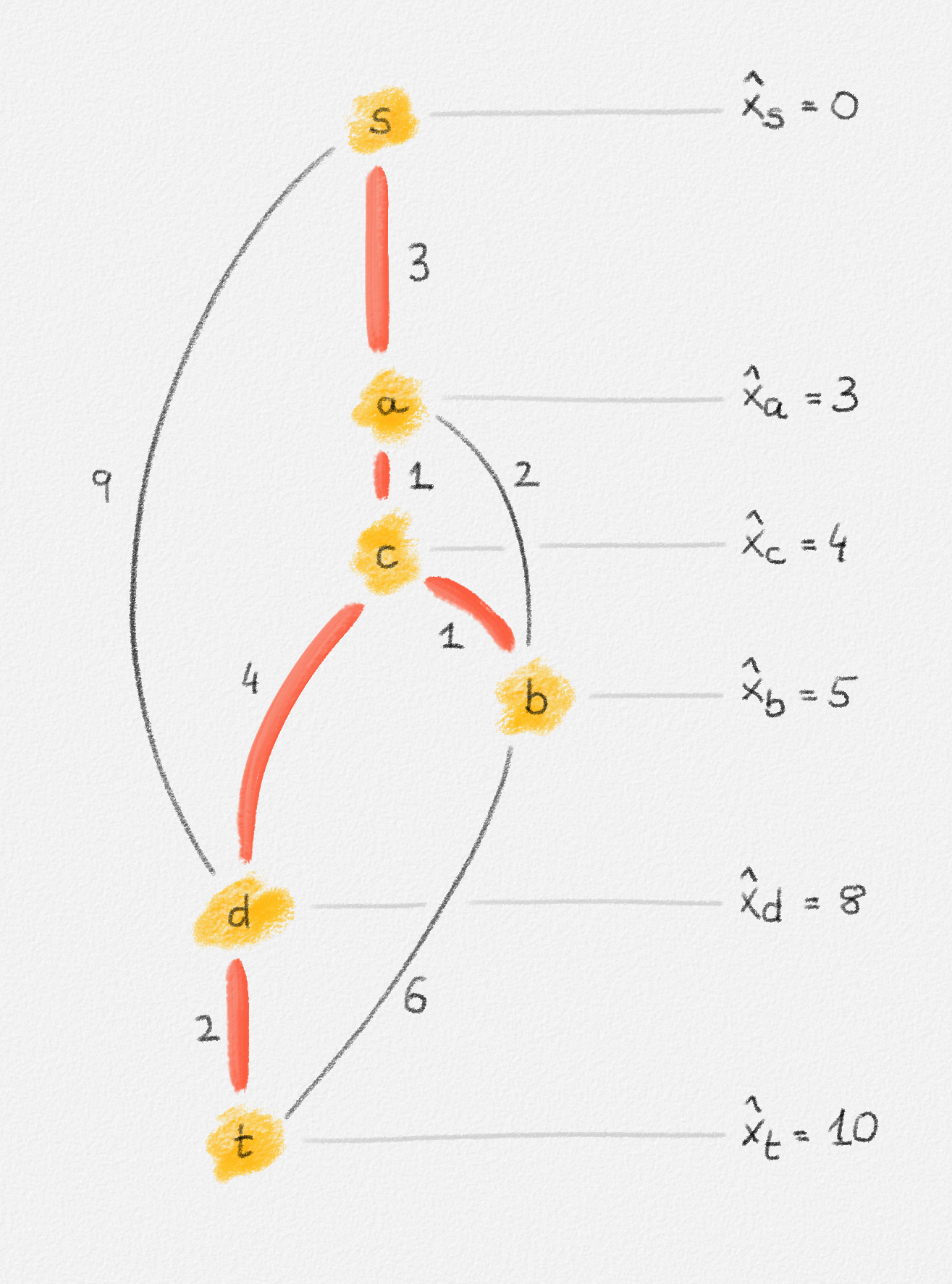
Figure 2.5: Illustration of the interpretation of (2.6) using the beads-and-string model. Holding the model from the vertex \(s\) makes each vertex hang the indicated distance below \(s\).

Thus, if \(\hat x_v\) represents how far below \(s\) we find \(v\), then gravity tries to maximize \(\sum_{v \in v} \hat x_v\). The condition that no string is being torn corresponds to the constraint that \(\hat x_v\) and \(\hat x_u\) can differ by at most \(w_{u,v}\), for every edge \((u,v)\) in the graph. Finally, once \(v\) has been pulled as far below \(s\) as possible by gravity, there must exist a path from \(s\) to \(v\) whose edges have been pulled tight. Otherwise, we would be able to pull \(v\) even farther away from \(s\). This path is a shortest path form \(s\) to \(v\), and its length is \(\hat x_v = \mathrm{dist}_{G,w}(s,v)\). The following lemma proves this claim formally.

Lemma 2.3: The optimal solution \(\hat x\) of the LP (2.6) satisfies \(\hat x_v = \mathrm{dist}_{G,w}(s,v)\) for all \(v \in V\).

Proof: Consider the subgraph \(H = (V,E') \subseteq G\) such that

\[E' = \bigl\{ (u,v) \in E \mid \hat x_v - \hat x_u = w_{u,v} \bigr\},\]

let \(S \subseteq V\) be the set of all vertices reachable from \(s\) in \(H\), and let \(T = V \setminus S\). See Figure 2.6.

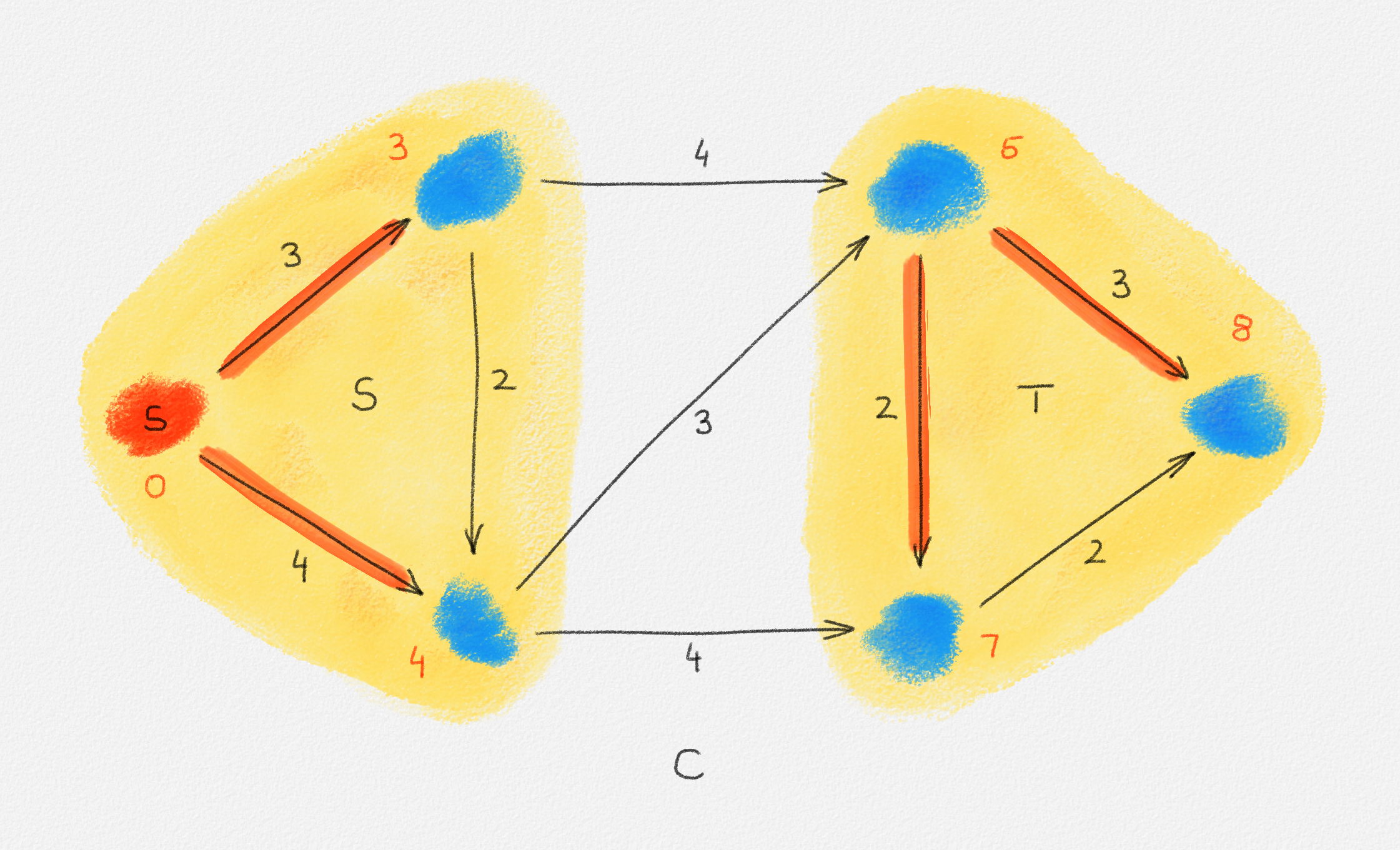
Figure 2.6: The sets \(S\) and \(T\) corresponding to the solution \(\hat x\) of (2.6) indicated by the red vertex labels. Black edge labels are the edge lengths. The red edges are tight and form the edge set of \(H\).

First we prove that \(T = \emptyset\), that is, that every vertex is reachable from \(s\) in \(H\).

Let

\[C = \{ (u,v) \in E \mid u \in S, v \in T \}.\]

Since every edge \((u,v) \in C\) has the property that \(u\) is reachable from \(s\) in \(H\) but \(v\) is not, it must satisfy \((u, v) \notin E'\) and, thus, \(\hat x_v - \hat x_u < w_{u,v}\). Therefore,

\[\delta = \min \bigl\{ w_{u,v} - \bigl(\hat x_v - \hat x_u\bigr) \mid (u,v) \in C \bigr\} > 0.\]

Now define a new solution \(\tilde x\) as

\[\tilde x_v = \begin{cases} \hat x_v & \text{if } v \in S\\ \hat x_v + \delta & \text{if } v \in T \end{cases}.\]

See Figure 2.7.

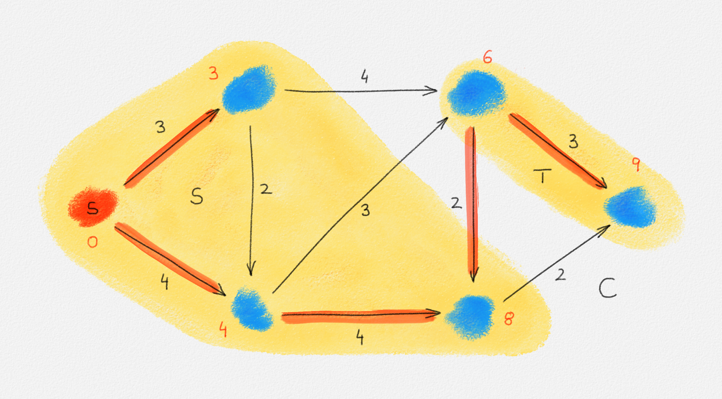
Figure 2.7: A solution \(\tilde x\) with a higher objective function value than the solution \(\hat x\) above. The new set \(S\) of vertices reachable from \(s\) is bigger.

Observe that \(s \in S\), so \(\tilde x_s = \hat x_s = 0\) because \(\hat x\) is a solution of (2.6).

For every edge \((u,v) \in E\), if \(v \in S\), then \(\tilde x_v = \hat x_v\) and \(\tilde x_u \ge \hat x_u\). Thus, \(\tilde x_v - \tilde x_u \le \hat x_v - \hat x_u \le w_{u,v}\).

If \(u, v \in T\), then \(\tilde x_v = \hat x_v + \delta\) and \(\tilde x_u = \hat x_u + \delta\). Thus, \(\tilde x_v - \tilde x_u = \hat x_v - \hat x_u \le w_{u, v}\).

Finally, if \(u \in S\) and \(v \in T\), then \(\tilde x_v = \hat x_v + \delta\) and \(\tilde x_u = \hat x_u\). Moreover, \((u, v) \in C\), so \(\delta \le w_{u, v} - \bigl(\hat x_v - \hat x_u\bigr)\). Therefore, \(\tilde x_v - \tilde x_u \le \hat x_v - \hat x_u + \delta \le w_{u,v}\).

This shows that \(\tilde x\) is a feasible solution of (2.6).

Next observe that \(\sum_{v \in V} \tilde x_v - \sum_{v \in V} \hat x_v = \delta|T|\). Since \(\tilde x\) is a feasible solution and \(\hat x\) is an optimal solution of (2.6), we have \(\sum_{v \in V} \tilde x_v - \sum_{v \in V} \hat x_v \le 0\), that is, \(T = \emptyset\) and \(S = V\).

The lemma now follows if every vertex \(v \in S\) satisfies \(\hat x_v = \mathrm{dist}_{G,w}(s,v)\). Let \(P = \langle v_0, \ldots, v_k \rangle\) be a path from \(s\) to \(v\) in \(H\). See Figure 2.8.

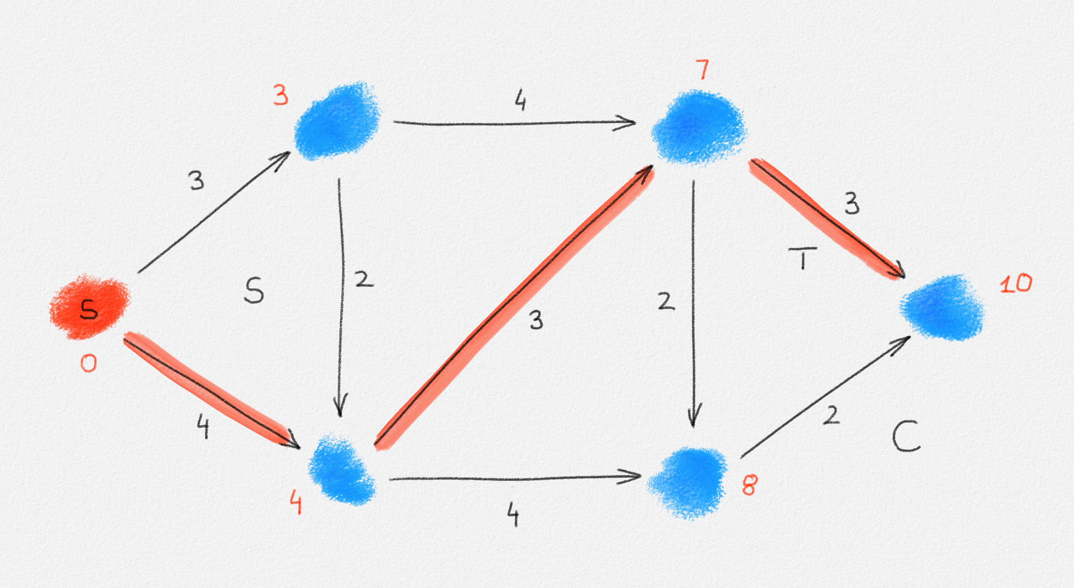
Figure 2.8: An optimal solution to (2.6) for the graph in Figure 2.6. The red path is a shortest path from \(s\) to the rightmost vertex.

Then \(\hat x_{v_0} = \hat x_s = 0\) and for \(1 \le i \le k\), \(\hat x_{v_i} = \hat x_{v_{i-1}} + w_{v_{i-1},v_i}\) because \(P\) is a path in \(H\). Thus,

\[\hat x_v = \hat x_{v_k} = \sum_{i=1}^k w_{v_{i-1},v_i} = w(P).\]

Since \(P\) is also a path from \(s\) to \(v\) in \(G \supseteq H\), this implies that

\[\hat x_v \ge \mathrm{dist}_{G,w}(s,v).\tag{2.7}\]

Conversely, for the shortest path \(\Pi_{G,w}(s,v) = \langle u_0, \ldots, u_\ell \rangle\) from \(s\) to \(v\) in \(G\), \(\hat x_{u_0} = \hat x_s = 0\) and, since \(\hat x\) is a solution of (2.6), \(\hat x_{u_i} \le \hat x_{u_{i-1}} + w_{u_{i-1},u_i}\) for all \(1 \le i \le \ell\). Thus,

\[\hat x_v = \hat x_{u_\ell} \le \sum_{i=1}^\ell w_{u_{i-1},u_i} = \mathrm{dist}_{G,w}(s,v).\tag{2.8}\]

Together, equations (2.7) and (2.8) show that \(\hat x_v = \mathrm{dist}_{G,w}(s,v)\). This finishes the proof. ▨

It may be useful to remind you at this point that our goal was to derive an LP formulation of the SSSP problem, that is, a linear program whose optimal solution consists of the distances from \(s\) to all vertices in \(G\). We proved that (2.6) is such an LP formulation. At this point, you may wonder how we go about finding such an optimal solution. We defer this discussion until Chapter 3, when we discuss the Simplex Algorithm. Our goal at this point is not to find optimal solutions to various optimization problems but to study how we can use linear programs as a mechanism to state these problems. We will later see that these formulations are useful because we can either solve the LPs using the Simplex Algorithm or the LP formulation sheds some light on the structure of the problem, which we can exploit in some algorithm we design to solve the problem.