2.2.1. The Single-Source Shortest Paths Problem

As a first example of the use of linear programs to model optimization problems, consider the single-source shortest paths problem.

Given a graph \(G = (V, E)\), a path from a vertex \(s\) to a vertex \(t\) is a sequence of vertices \(P = \langle v_0, \ldots, v_k \rangle\) such that \(v_0 = s\), \(v_k = t\), and there exists an edge \(e_i = (v_{i-1},v_i) \in E\) for all \(1 \le i \le k\). See Figure 2.2.

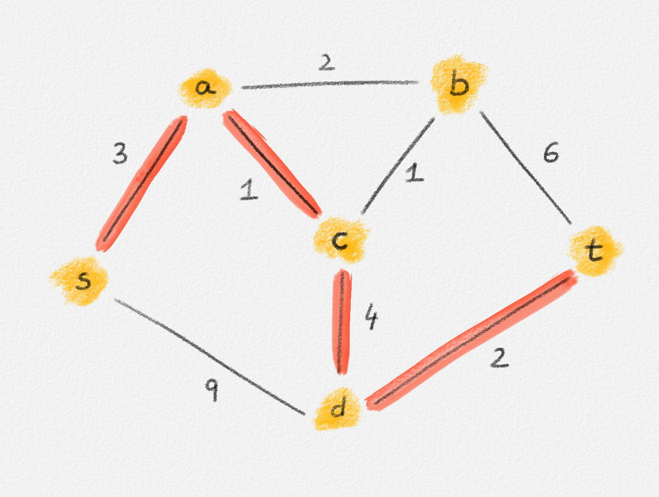
Figure 2.2: The red path \(\langle s, a, c, d, t\rangle\) is a shortest path from \(s\) to \(t\) of length \(10\). \(\langle s, d, t\rangle\) is another path from \(s\) to \(t\), but it is not a shortest path because its length is \(11\).

Depending on the context, \(P\) may be viewed as the sequence of its vertices, the sequence of its edges \(\langle e_1, \ldots, e_k \rangle\) or the alternating sequence of both \(\langle v_0, e_1, v_1, \ldots, e_k, v_k \rangle\).

A path \(P\) from a vertex \(s\) to a vertex \(t\) is a cycle if \(s = t\). See Figure 2.3.

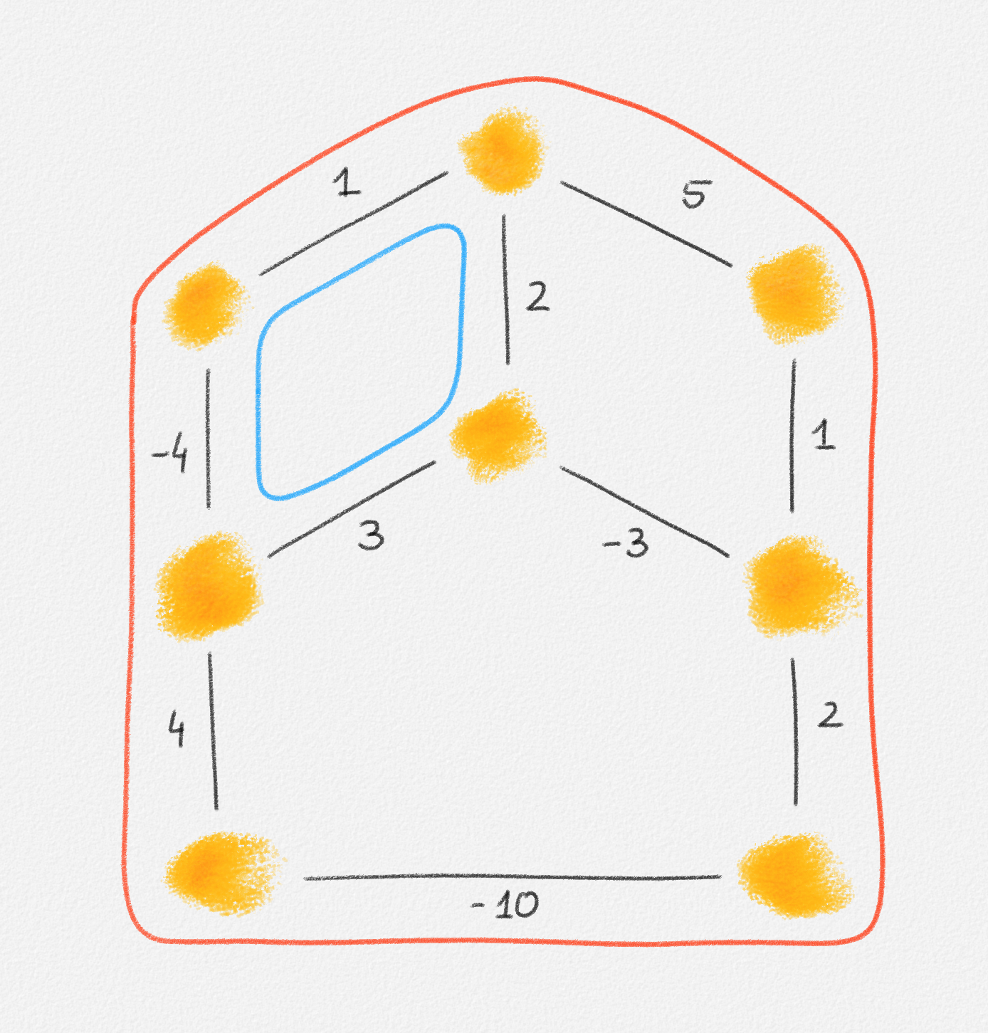
Figure 2.3: The red and blue paths are cycles. The red one is a negative cycle of weight \(-1\). The blue one is not a negative cycle; its weight is \(2\).

An edge-weighted graph is a pair \((G,w)\) consisting of a graph \(G = (V,E)\) and an assignment \(w : E \rightarrow \mathbb{R}\) of weights to its edges.

The weight or length of a path \(P\) in an edge-weighted graph \((G,w)\) is the total weight of all edges in \(P\):

\[w(P) = \sum_{e \in P} w_e\]

A shortest path from a vertex \(s \in V\) to a vertex \(t \in V\) is a path \(\Pi_{G,w}(s,t)\) from \(s\) to \(t\) in \(G\) such that every path \(P\) from \(s\) to \(t\) in \(G\) satisfies \(w(P) \ge w(\Pi_{G,w}(s,t))\).

The distance from \(s\) to \(t\) is

\[\mathrm{dist}_{G,w}(s,t) = w(\Pi_{G,w}(s,t)).\]

Shortest paths in an edge-weighted graph \((G,w)\) are well defined only if there are no negative cycles in \((G,w)\), where

A negative cycle is a cycle \(C\) in \(G\) with \(w(C) < 0\).

Indeed, if there exists a path from \(s\) to \(t\) that includes a vertex in some negative cycle \(C\), then it is possible to generate arbitrarily short paths from \(s\) to \(t\) by including sufficiently many passes through \(C\) in the path.

The single-source shortest paths problem is to compute the distance from some source vertex \(s\) to every vertex \(v \in V\):

Single-source shortest paths problem (SSSP): For an edge-weighted graph \((G,w)\) and a source vertex \(s \in V\), compute \(\mathrm{dist}_{G,w}(s, v)\) for all \(v \in V\).

In general, the goal is to find the actual shortest paths \(\Pi_{G,w}(s,v)\), not only the distances \(\mathrm{dist}_{G,w}(s,v)\). By the following two exercises, computing the distances is the hard part.

Exercise 2.1: In general, there may be more than one shortest path between two vertices \(s\) and \(t\) in a connected edge-weighted graph \((G, w)\). Prove that it is possible to choose a particular shortest path \(\Pi_{G,w}(s, v)\) for each vertex \(v \in V\) such that the union of these shortest paths is a tree. This tree is called a shortest path tree.

Exercise 2.2: Show that finding the shortest paths from a vertex \(s\) to all vertices \(v\) in an edge-weighted graph \((G, w)\) is no harder than computing the distances from \(s\) to all vertices in \(G\). Specifically, if \(d : V \rightarrow \mathbb{R}\) is a labelling of the vertices of \(G\) such that \(d_v = \mathrm{dist}_{G,w}(s,v)\) for all \(v \in V\), show how to compute a shortest path tree \(T\) with root \(s\) in \(O(n + m)\) time.