5.2.2.2. The Algorithm

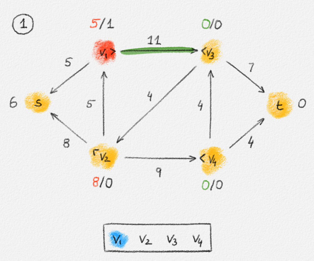
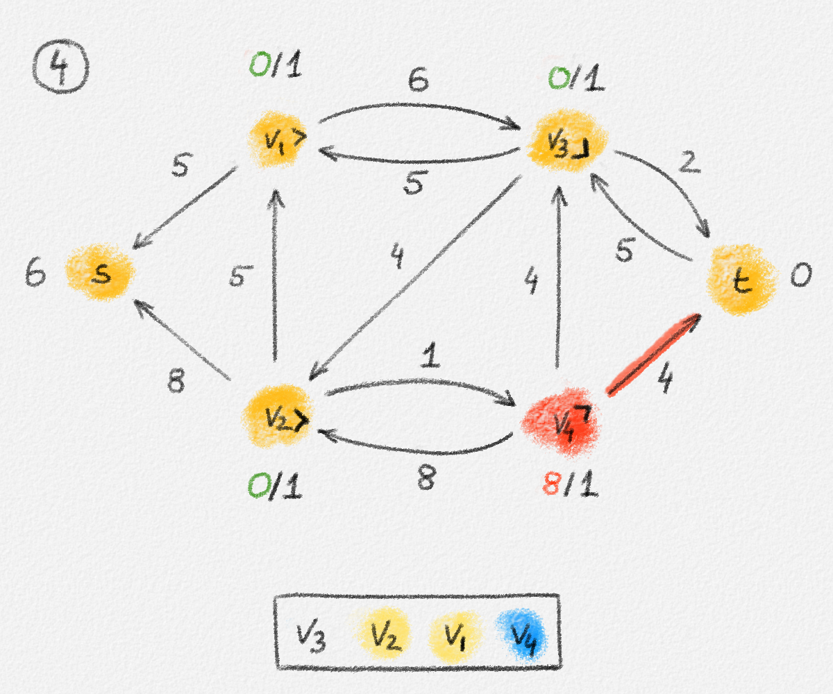
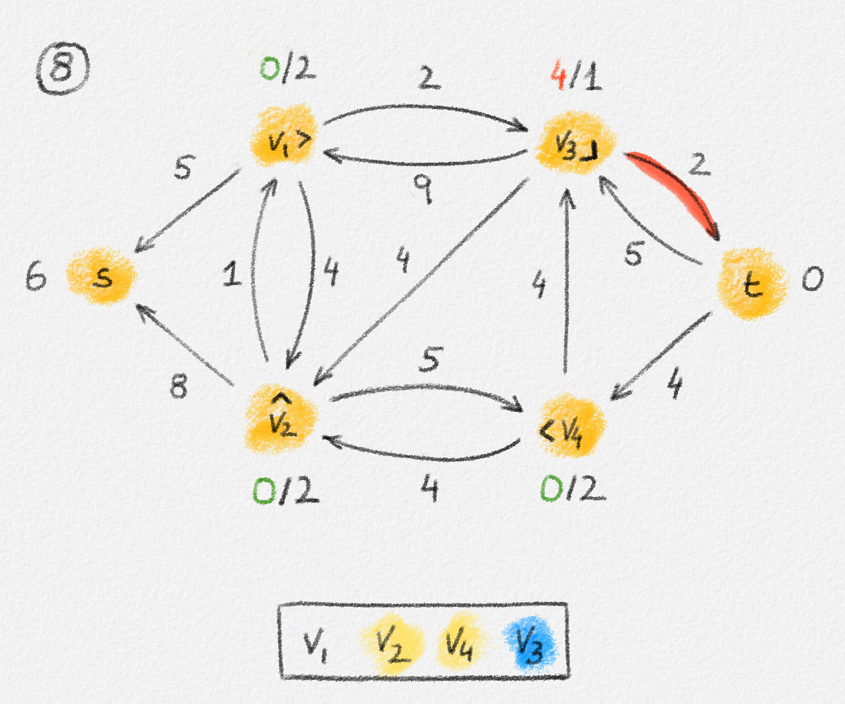
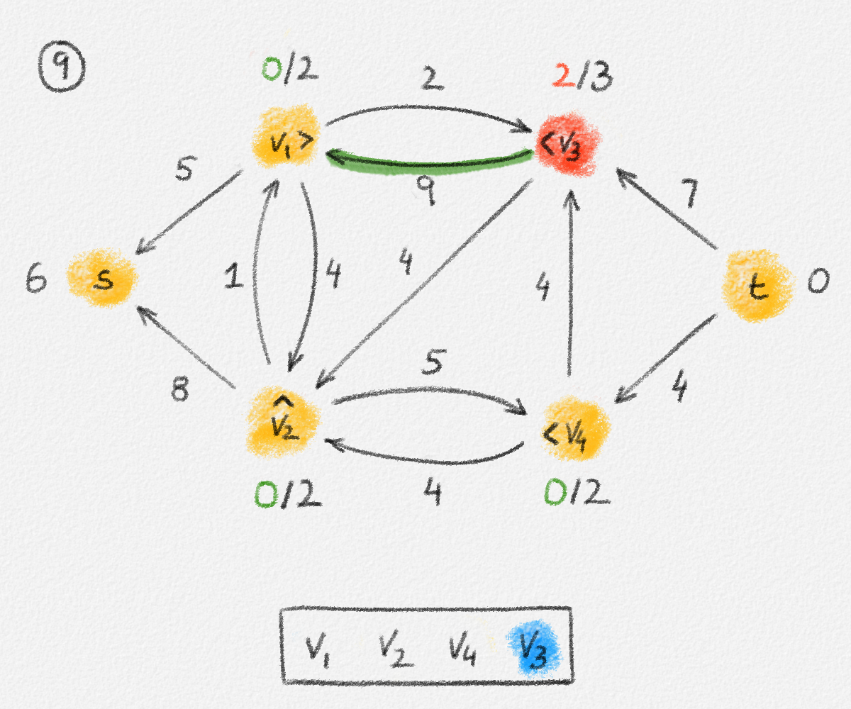
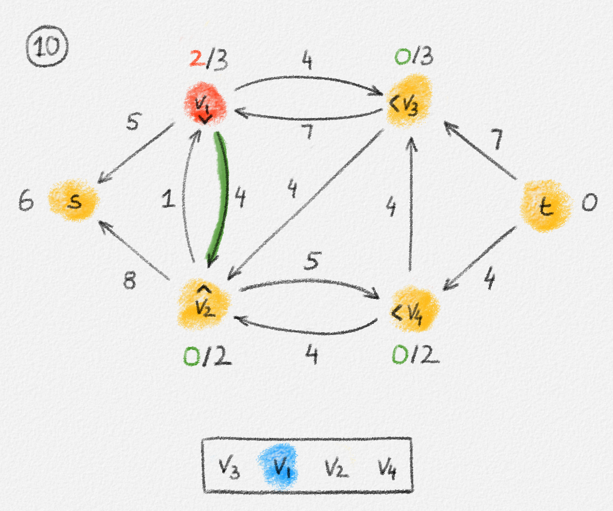
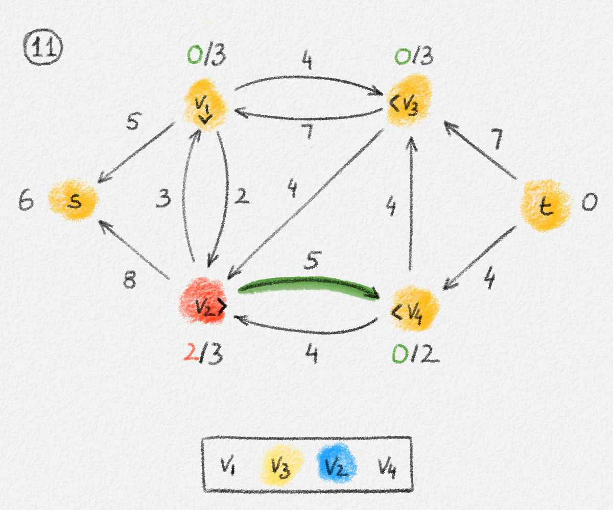
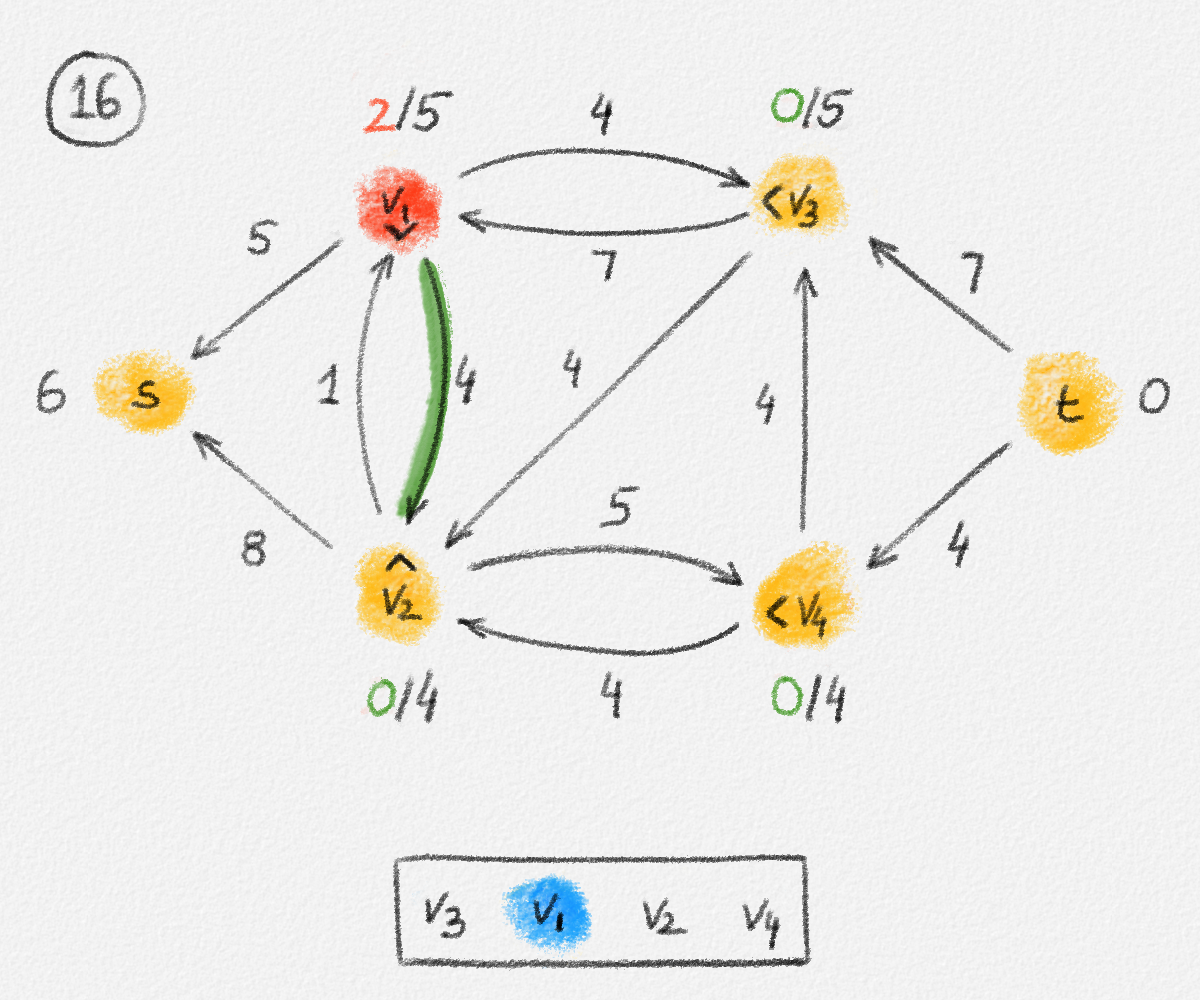
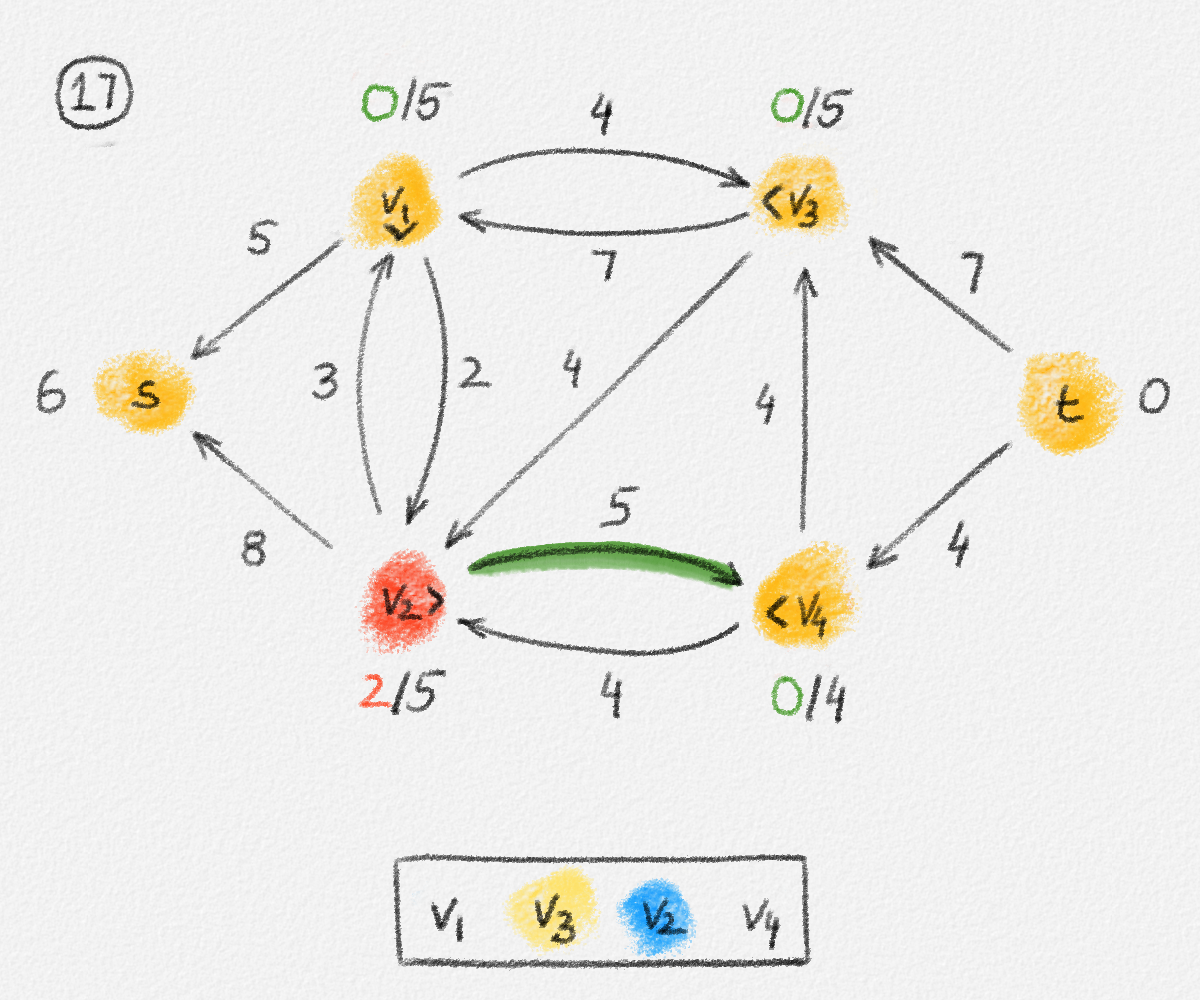
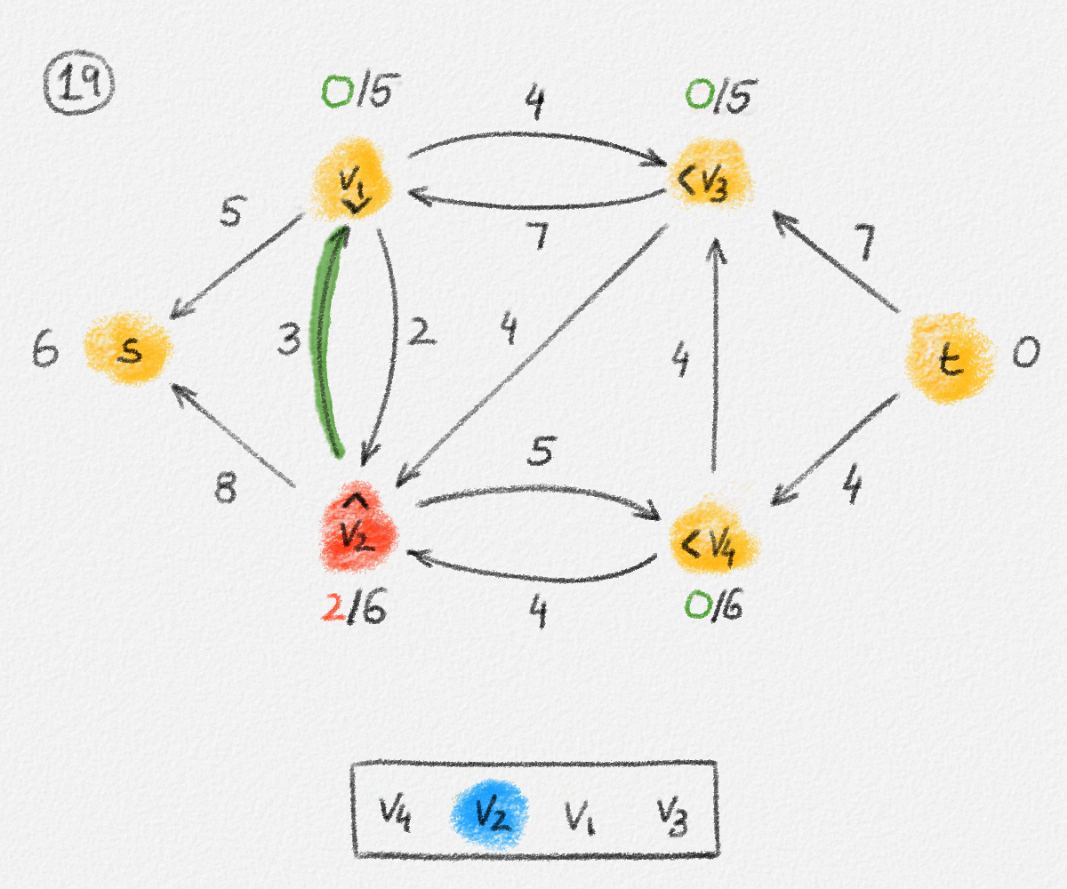
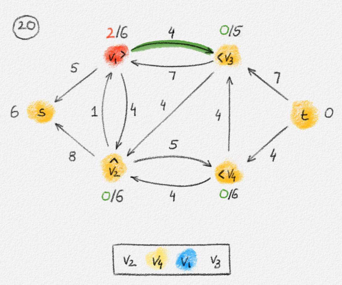
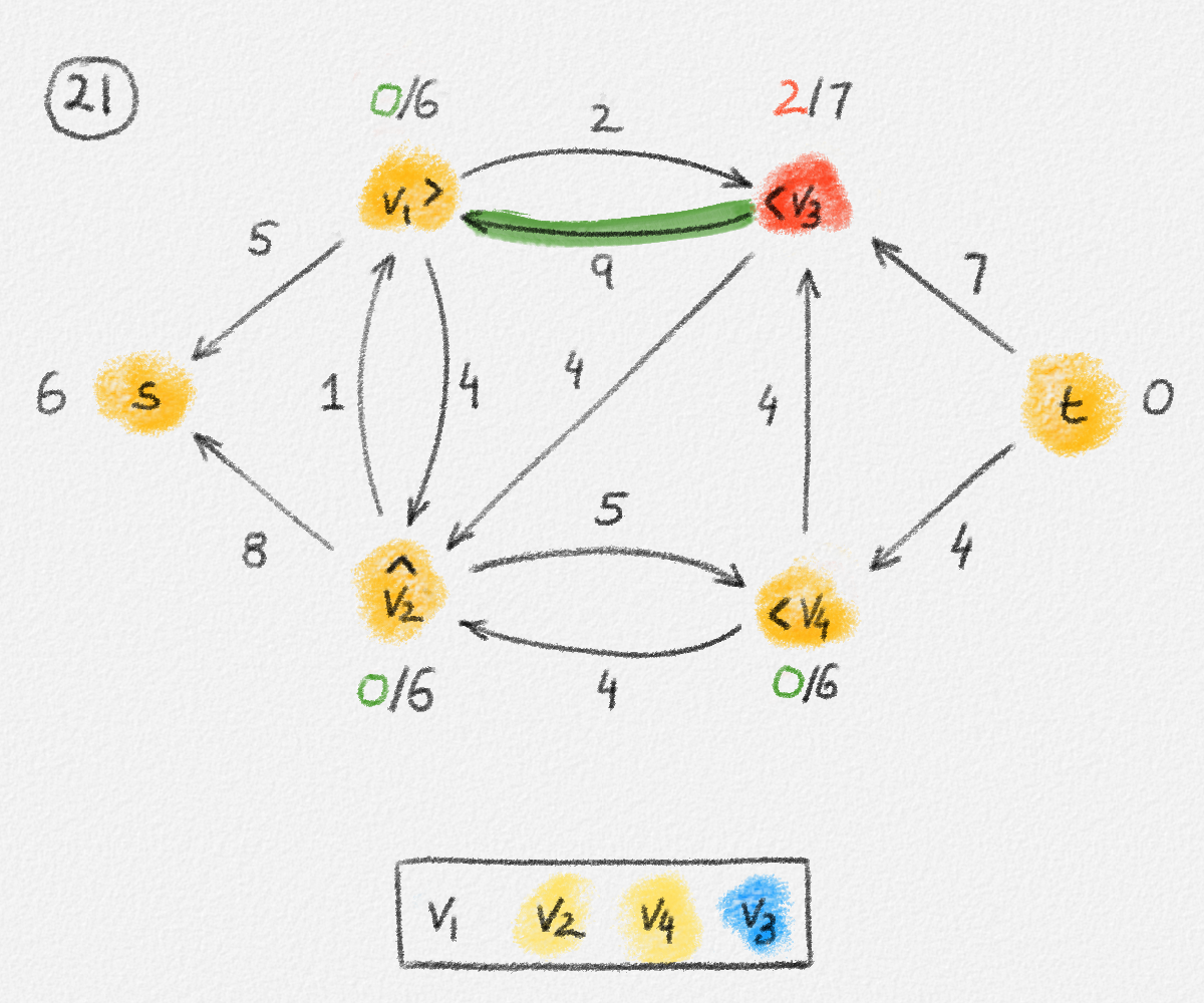
The relabel-to-front algorithm (procedure RelabelToFront below) derives its name from the manner in which it maintains the list of vertices to be discharged. An illustration of this algorithm is given in Figure 5.17.

PROCEDURE \(\boldsymbol{\textbf{RelabelToFront}(G, u, s, t)}\):

---

INPUT:

• A directed graph \(G = (V, E)\)
• A capacity labeling \(u : E \rightarrow \mathbb{R}^+\) of its edges
• A source vertex \(s\)
• A sink vertex \(t\)

OUTPUT:

• A maximum \(st\)-flow \(f : E \rightarrow \mathbb{R}^+\)

---

1.     FOR every vertex \(x \in V\) DO
2.         \(h_x = 0\)
3.     \(h_s = n\)
4.     FOR every edge \(e \in E\) DO
5.         \(f_e = 0\)
6.     FOR every out-neighbour \(y\) of \(s\) in \(G\) DO
7.         \(f_{s,y} = u_{s,y}\)
8.     \(L = V\)
9.     \(x = \textrm{HEAD}(L)\)
10.     WHILE \(x \ne \textrm{NULL}\) DO
11.         \(h_x' = h_x\)
12.         \((f, h) = \textbf{Discharge}(G, u, f, h, x)\)
13.         IF \(h_x > h_x'\) THEN
14.             Move \(x\) to the front of \(L\)
15.         \(x = \textrm{NEXT}(x)\)
16.     RETURN \(f\)

The algorithm maintains the vertices of \(G\) in a doubly-linked list \(L\), initially stored in no particular order, and initializes \(x\) to be the first vertex in \(L\). Then, as long as \(x \ne \textrm{NULL}\), it calls \(\boldsymbol{\textbf{Discharge}(x)}\) to ensure that \(x\)'s excess is zero and then advances \(x\) to the next vertex in \(L\). If \(\boldsymbol{\textbf{Discharge}(x)}\) relabels \(x\), which can be detected by observing an increase in \(x\)'s height \(h_x\), then the algorithm moves \(x\) to the front of the list \(L\) before advancing to \(x\)'s successor, that is, the new current vertex \(x\) after the current operation is the second vertex in \(L\) even if \(x\) was fairly close to the end of \(L\) before the \(\boldsymbol{\textbf{Discharge}(x)}\) operation. Thus, the algorithm may iterate over the vertices in \(L\) several times. Can this process continue forever or will the algorithm eventually reach a state when \(x \ne \textrm{NULL}\), so the algorithm terminates? This is the question we answer in the next section.

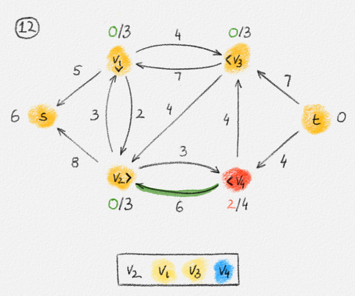
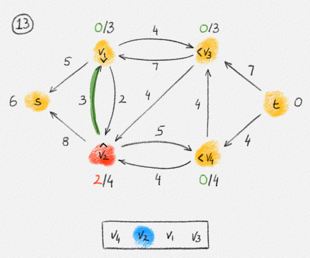
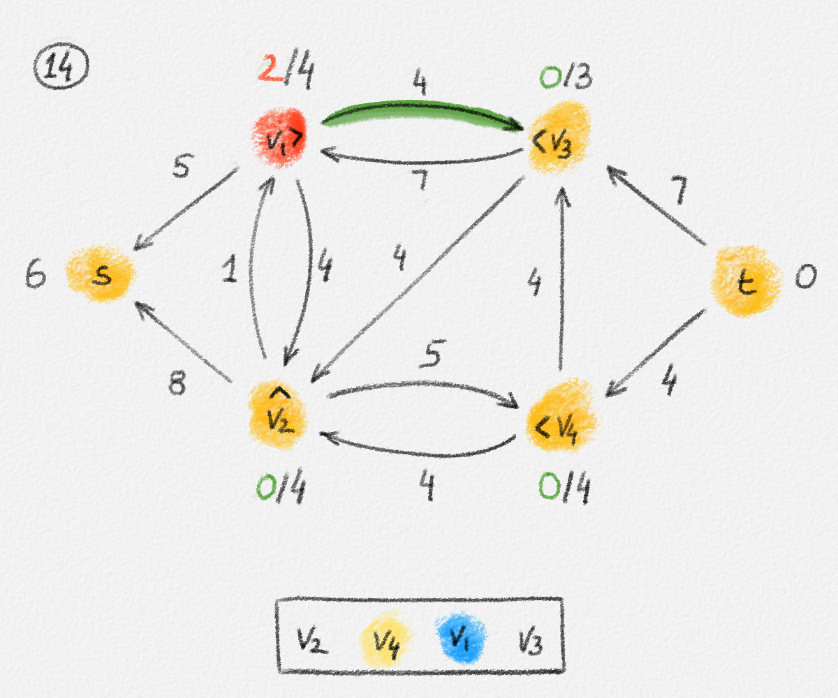
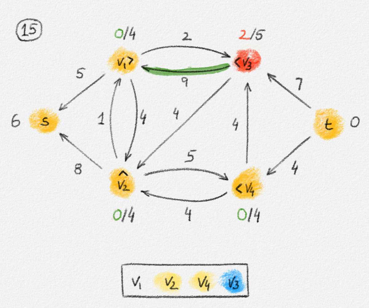
Figure 5.17: Illustration of an application of the relabel-to-front algortihm to the network in Figure 5.1. The circled numbers indicate the iteration number. We assume that initially, \(L = \langle v_1, v_2, v_3, v_4\rangle\) and that the vertices in each vertex's neighbour list are sorted by the relation \(s < v_1 < v_2 < v_3 < v_4 < t\). For the different iterations of the algorithm, only the residual network is shown. Edge labels are edge capacities. Black node labels are node heights. Coloured node labels are node excesses, shown in red if positive, and in green if zero. In each figure, the edge used to push flow to a neighbour is shown in red if it is a saturating push, and in green if it is a non-saturating push. If the tail of the edge was relabelled to allow this push to happen, this tail node is shown in red. Every node \(u\) points to its current neighbour \(\textrm{CUR}(u)\) using a small chevron. Finally, for each iteration, the current state of the list \(L\) is shown below the network. The current node is shaded blue. Nodes that were skipped to reach this current node because they have no excess are shaded yellow. The final network on the last row shows the computed flow.