7.5.2.1. A Single Iteration

In the proof of Lemma 7.11, we discussed how to find an augmenting path for a given matching \(M\) by constructing a maximum alternating forest \(F\) with all unmatched vertices in \(U\) as its roots and testing whether \(F\) contains an unmatched vertex \(w \in W\). If such a vertex \(w \in W\) exists, then the path \(P_w\) from \(w\) to \(r_w\) in \(F\) is an augmenting path for \(M\).

Each iteration of the Hungarian algorithm employs the exact same strategy, except that we construct \(F\) by applying alternating BFS only to the tight subgraph of \(G\), the subgraph \(G^\pi\) of \(G\) containing all tight edges with respect to the current potential function \(\pi\). We use \(F^\pi\) to refer to an alternating forest of \(G^\pi\) whose roots are all unmatched vertices in \(U\), and we may also say that \(F^\pi\) is an alternating forest with respect to \(\boldsymbol{\pi}\). If we do find an augmenting path \(P_w\) in \(F^\pi\), it is a tight augmenting path, and \(M \oplus P_w\) is a matching composed of tight edges and of size \(|M \oplus P_w| = |M| + 1\), that is, replacing \(M\) with \(M \oplus P_w\) makes progress towards a perfect matching and maintains complementary slackness. As explained before, the iteration is the last iteration in its phase in this case because we have achieved the goal of the current phase, which was to grow the matching by one edge.

The more interesting question is how to adjust \(\pi\) when we fail to find a tight augmenting path using this strategy:

In this case, we define four sets \(X\), \(\bar X\), \(Y\), and \(\bar Y\). \(X \subseteq U\) is the set of all vertices in \(U\) that belong to \(F_\pi\) and \(\bar X = U \setminus X\). In other words, \(X\) is the set of all vertices in \(U\) that are reachable from unmatched vertices in \(U\) via tight alternating paths. Similarly, \(Y \subseteq W\) is the set of all vertices in \(W\) that belong to \(F\) and \(\bar Y = W \setminus Y\). Thus, again, \(Y\) is the set of all vertices in \(W\) that are reachable from unmatched vertices in \(U\) via tight alternating paths. This is illustrated in Figure 7.13.

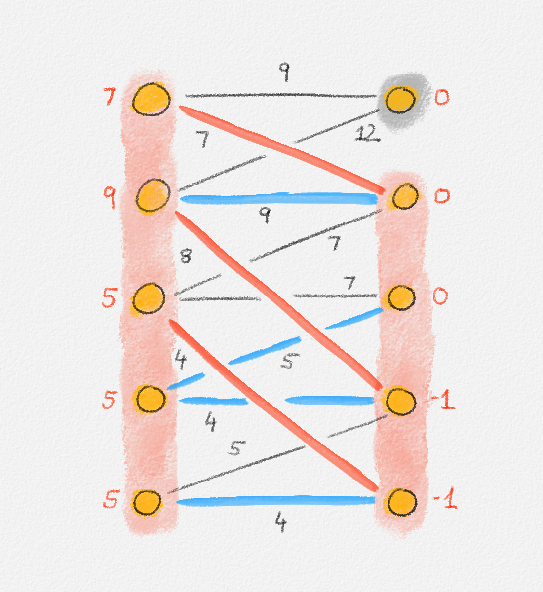
Figure 7.13: The two bottom vertices on the left side (\(U\)) are unmatched. The vertices shaded pink are the ones in \(X\) and \(Y\), that is, the ones reachable from one of these two vertices via alternating paths. The vertices shaded grey are the ones in \(\bar X\) and \(\bar Y\), that is, the ones not reachable from one of these two vertices via alternating paths. In this example, \(\bar X = \emptyset\). The red edges are in the current matching. The blue edges are unmatched edges in \(F^\pi\). In particular, they are tight. The black edges are not in \(F^\pi\). In this example, none of the black edges is tight. In general, however, there can be tight edges that are not included in \(F^\pi\).

Let

\[\delta = \min_{u \in X, w \in \bar Y} (c_{u,w} - \pi_u - \pi_w),\]

and define a new potential function \(\pi'\) as

\[\pi_v' = \begin{cases} \pi_v + \delta & \text{if } v \in X\\ \pi_v - \delta & \text{if } v \in Y\\ \pi_v & \text{otherwise}. \end{cases}\]

We replace our potential function \(\pi\) with \(\pi'\) and then start another iteration. As we will show next, every edge in \(M\) remains tight with respect to this new potential function \(\pi'\), and the alternating forest \(F^{\pi'}\) contains all vertices in \(Y\) as well as at least one vertex in \(\bar Y\). Thus, after adjusting \(\pi\) in this fashion at most \(n\) times, \(F\) contains all vertices in \(W\). As long as the current matching \(M\) is not a perfect matching, there exists an unmatched vertex in \(W\), that is, once \(F^\pi\) contains all vertices in \(W\), there must exist an augmenting path in \(F^\pi\), and this augmenting path is tight. This is the argument why each phase consists of at most \(n\) iterations that adjust \(\pi\) as just described, followed by an iteration that increases the size of \(M\).

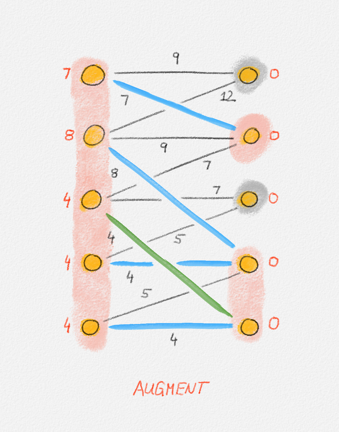
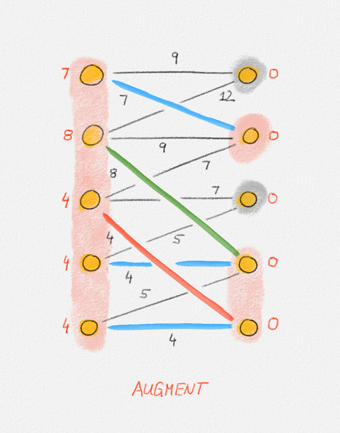
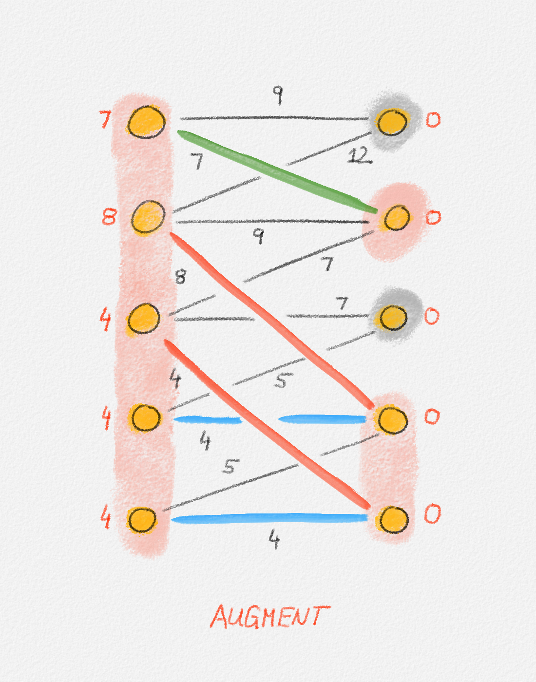
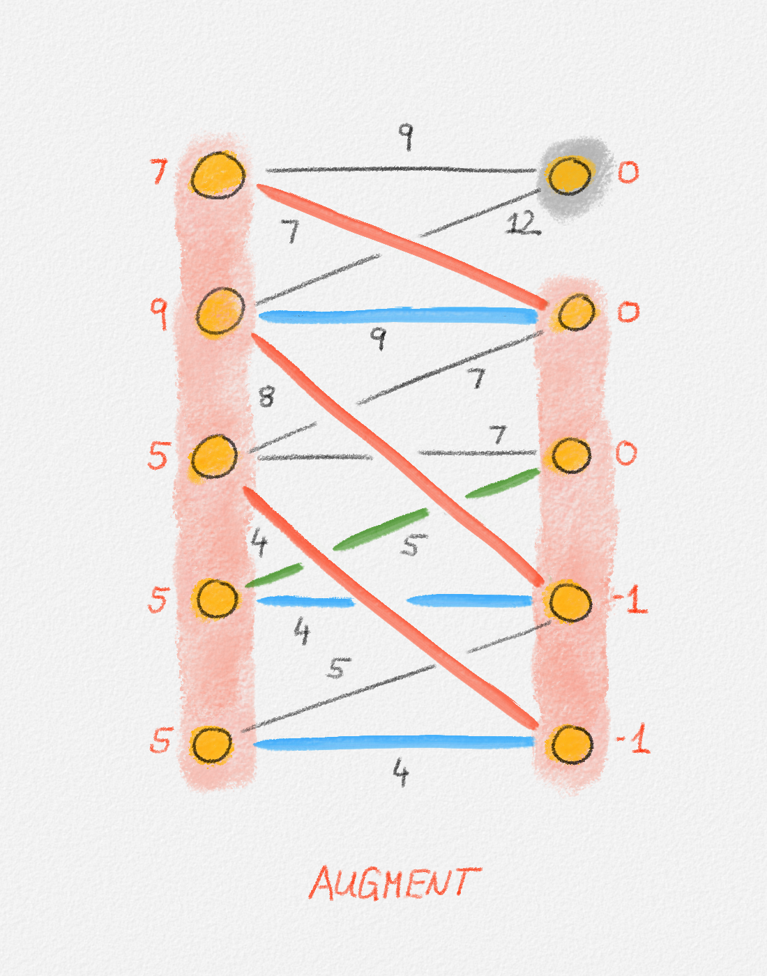
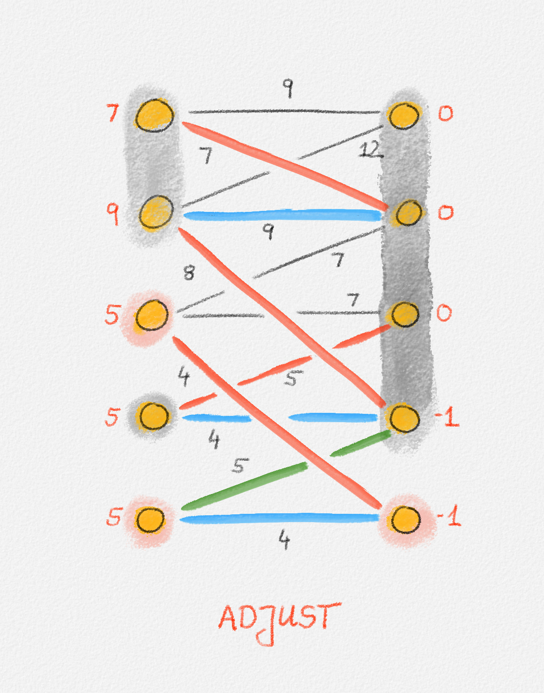
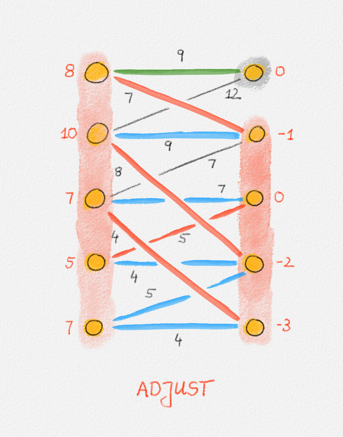
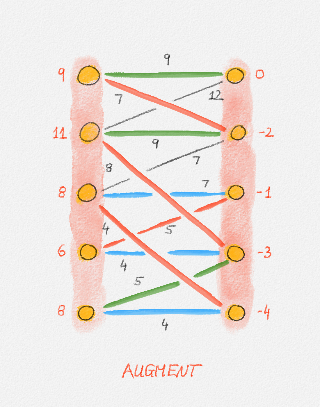
Figure 7.14 illustrates a complete run of the Hungarian Algorithm. Note that the graph in Figure 7.14 is not complete. We can apply the Hungarian Algorithm also to incomplete bipartite graphs, only the algorithm is no longer guaranteed to succeed because the graph may not have a perfect matching.

Phase 1

Phase 2

Phase 3

Phase 4

Phase 5

Final matching

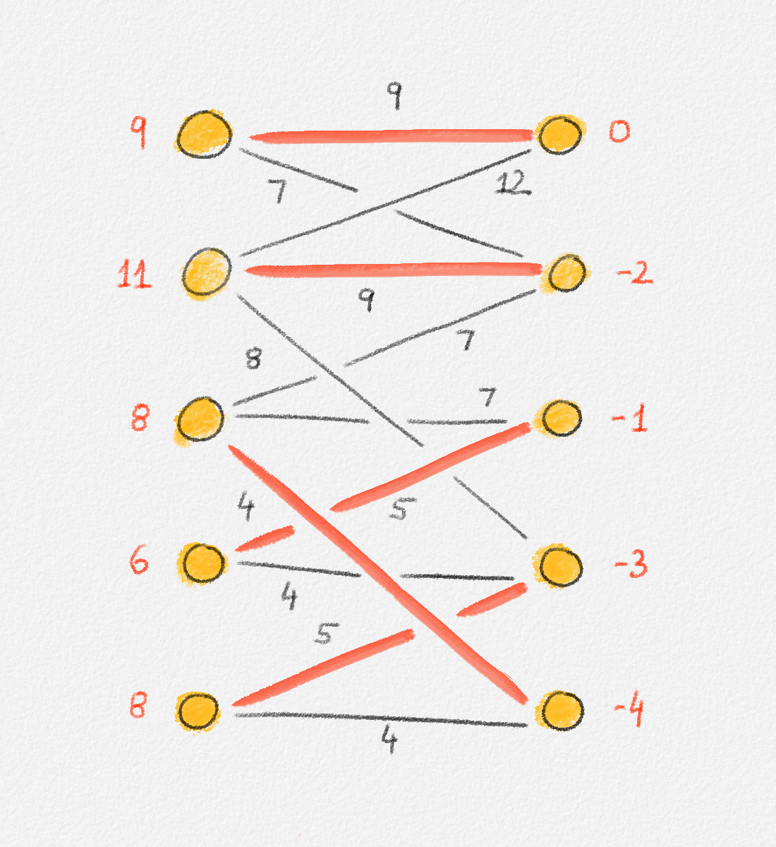
Figure 7.14: Illustration of a full run of the Hungarian algorithm. In this case, the algorithm runs for 5 phases. The final iteration in each phase grows the matching. If the phase has more than one iteration, the iterations before the final iteration adjust the potential function to create more tight edges that can be followed to obtain a larger alternating forest \(F^\pi\). In each figure, red vertex labels are the vertex potentials. Black edge labels are the edge costs. \(X\) and \(Y\) are shaded pink. \(\bar X\) and \(\bar Y\) are shaded grey. Blue edges are tight, black edges are not. Red edges are the edges in the current matching and are also tight. In an augmentation iteration, the augmenting path used to grow the matching is the one composed of the green edges and possibly red matching edges connecting them. (The only phase in this example where the augmenting path has more than one edge is Phase 5.) In an adjustment iteration, the green edge is the tightest edge between \(X\) and \(\bar Y\). The vertex potentials of the vertices in \(X\) and \(Y\) are adjusted by the slack of this edge. The last figure shows the final matching and potential function computed by the algorithm. The matching is clearly a perfect matching. The potential function is a valid potential function and all edges in the matching are tight with respect to this potential function, so the matching is a minimum-weight perfect matching.