7.1. Definitions

Matching problems are also known as assignment problems because the basic problem is to pair entities. Consider for example a set of compute jobs to be run and a set of machines they can be run on. Each machine completes each job in a particular amount of time based on the demands of the job in terms of CPU speed, memory bandwidth, and amount of memory available and the machine's specifications. You are renting these machines from Amazon at some cost per hour. In this scenario, it is not hard to imagine that the cost of running each job can differ significantly from machine to machine. We want to assign jobs to available machines so that the total cost of running all jobs is minimized.

We can model this as a bipartite graph \(G\) whose vertex set is the union of two sets \(J\) and \(M\) representing the jobs and machines, respectively.

A graph \(G = (V, E)\) is bipartite if the vertex set \(V\) can be partitioned into two disjoint subsets \(U\) and \(W\)—\(V = U \cup W\) and \(U \cap W = \emptyset\)—such that every edge of \(G\) has one endpoint in \(U\) and the other in \(W\). See Figure 7.1.

We usually write \(G = (U, W, E)\) if \(G\) is bipartite to make the partition of \(V\) into subsets \(U\) and \(W\) explicit.

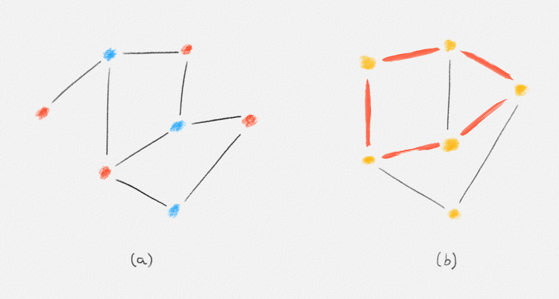
Figure 7.1: The graph in (a) is bipartite because every edge has a red endpoint and a blue endpoint. In other words, the partition of the vertex set into the set \(U\) containing all red vertices and the set \(W\) containing all blue vertices proves that the graph is bipartite. By Exercise 7.2, the graph in (b) is not bipartite because of the odd cycle formed by the red edges.

Back to scheduling jobs on machines. If a job \(j \in J\) can run on a machine \(m \in M\) (some jobs may not be possible to run on a given machine at all, for example, if the job has high memory requirements and the machine has too little memory), then there is an edge \((j, m) \in G\) with weight equal to the cost of running job \(j\) on machine \(m\). If we assume that we want to run every job on a different machine, our goal is to pick a subset of the edges in \(G\) such that no two edges share an endpoint (no two jobs run on the same machine and no job can be split over multiple machines), every vertex in \(J\) is the endpoint of a chosen edge (we run every job), and the total weight of the chosen edges is minimized.

A set \(M\) of edges in a graph such that no two edges in \(M\) share an endpoint is called a matching. For every edge \((x,y) \in M\), we call \(x\) and \(y\) mates. See Figure 7.2.

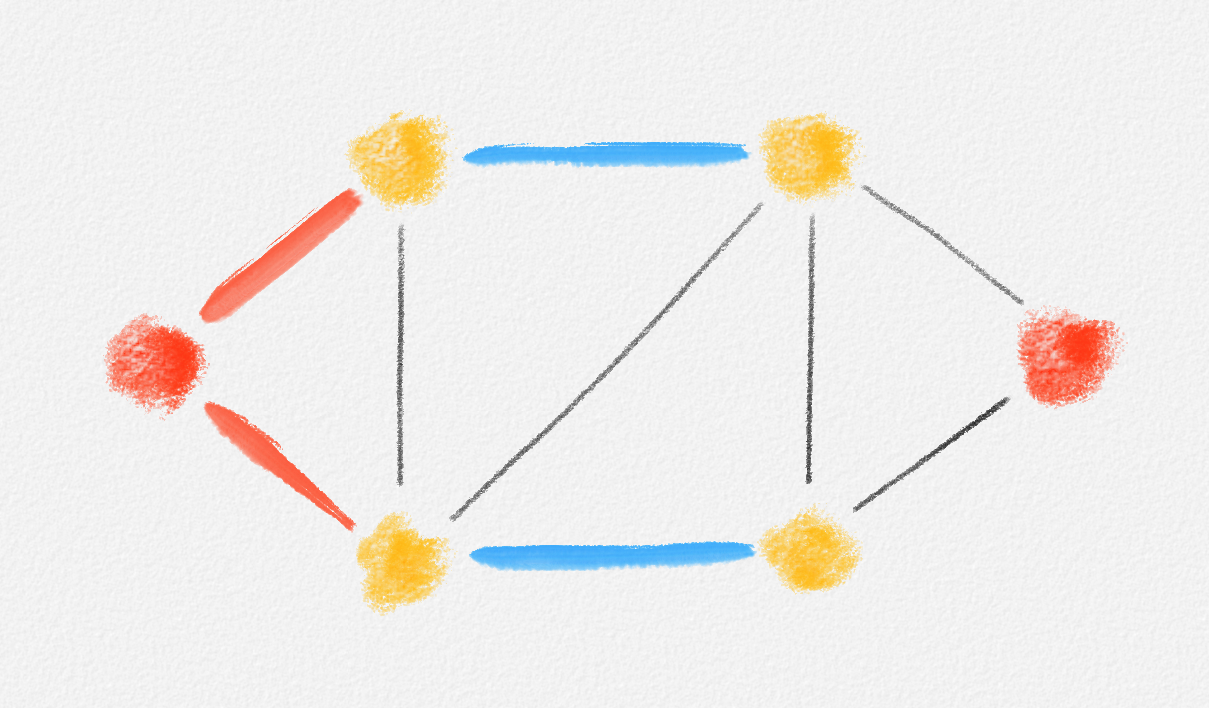
Figure 7.2: The blue edges form a matching, as these edges do not have any endpoints in common. The red edges do not form a matching, as they share an endpoint.

Throughout this chapter, we refer to a vertex \(x\) of a graph \(G\) as matched by a matching \(M\) if \(x\) is an endpoint of an edge in \(M\); otherwise, \(x\) is unmatched by \(M\). If the matching is clear from the context, we will refer to vertices simply as matched or unmatched, without specifying the matching. We also refer to edges as matched or unmatched depending on whether they belong to \(M\).

If every vertex of \(G\) is the endpoint of an edge in \(M\), then \(M\) is called a perfect matching. See Figure 7.3.

Figure 7.3: The blue edges in Figure 7.2 do not form a perfect matching because the two red vertices are unmatched. The red edges in this figure do form a perfect matching because every vertex is an endpoint of a red edge. The blue edges in this figure also form a perfect matching. The blue edges do not form a minimum-weight perfect matching because the red edges have lower total cost. You can check that there is no perfect matching of lower cost than the red edges, so the red edges form a minimum-weight perfect matching.

In the above scenario of scheduling jobs on machines, if the number of jobs equals the number of available machines, then the requirement that every job has an incident edge in the matching implies that every machine also has an incident edge in the matching. Thus, we are looking for a minimum-weight perfect matching:

Given a graph \(G = (V, E)\) and a cost function \(c : E \rightarrow \mathbb{R}\), a minimum-weight perfect matching is a perfect matching \(M\) such that no perfect matching of \(G\) has lower cost. See Figure 7.3.

Such a matching may not exist since there may be pairs of vertices not connected by an edge. Thus, we may also consider the simpler problem of deciding whether a perfect matching exists. This decision problem can be generalized to the maximum-cardinality matching problem, which is to find a matching containing as many edges as possible.

Given a graph \(G\), a maximum-cardinality matching is a matching \(M\) of \(G\) such that no matching of \(G\) contains more edges than \(M\).

Observation 7.1: A matching \(M\) of an \(n\)-vertex graph \(G\) is a perfect matching if and only if it has size \(\frac{n}{2}\).

In the same way we went from the minimum-weight perfect matching problem to the simpler problem of finding a perfect matching, we can generalize the maximum-cardinality matching problem to the maximum-weight matching problem, which asks us to find a matching of maximum weight.

Given a graph \(G = (V, E)\) and a cost function \(c : E \rightarrow \mathbb{R}\), a maximum-weight matching is a matching \(M\) such that no matching of \(G\) has greater cost. The cost of a matching is the total cost of its edges: \(c(M) = \sum_{e \in M} c_e\).

Note that a maximum-weight matching may contain fewer edges than a maximum-cardinality matching for the same graph if the edge costs in the graph vary sufficiently. An example is shown in Figure 7.4.

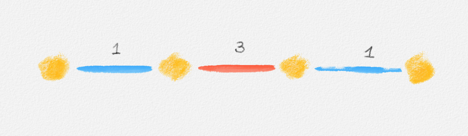
Figure 7.4: The blue edges are a maximum-cardinality matching: The matching is perfect, so there cannot be any bigger matching. It is not a maximum-weight matching because the red edge has a greater cost than the total cost of the two blue edges. The set containing only the red edge is a maximum-weight matching but not a maximum-cardinality matching because the matching consisting of the blue edges contains more edges.

Exercise 7.1: Prove that it is possible to adjust the costs in a weighted graph so that a maximum-weight matching with respect to the adjusted costs is

• A matching of maximum cost (with respect to the original costs) among all maximum-cardinality matchings of the graph or

• A matching of maximum cardinality among all maximum-weight matchings (with respect to the original costs) of the graph.

The final generalization we consider is to drop the requirement that the given graph be bipartite. Many natural applications of matching problems work with bipartite graphs and, as we will see, solving matching problems on bipartite graphs can be significantly easier than on arbitrary graphs. Nevertheless, it is useful to be able to find various kinds of matchings in arbitrary graphs, particularly as a building block for other algorithms.

Since bipartite graphs play a central role throughout most of this chapter, here are two exercises that help you get more comfortable thinking about the structure of bipartite graphs:

Exercise 7.2: Prove that a graph is bipartite if and only if it contains no odd cycle (cycle of odd length).

Exercise 7.3: Show that if a bipartite graph \(G = (V, E)\) is connected, then there exists exactly one partition of \(V\) into two disjoint subsets \(U\) and \(W\) such that every edge has one endpoint in \(U\) and the other in \(W\). Prove that in general, a non-empty bipartite graph with \(k\) connected components has \(2^{k-1}\) such partitions of its vertex set into subsets \(U\) and \(W\).