2.5.2. An ILP Formulation of the MST Problem With Integrality Gap 1

The following extension of (2.9) finally is an ILP whose LP relaxation has an optimal integral solution:

\[\begin{gathered} \text{Minimize } \sum_{e \in E} w_e x_e\\ \begin{aligned} \text{s.t. } \phantom{\displaystyle\sum_{\substack{(u,v) \in E\\u,v \in S}} x_{u,v}} \llap{\displaystyle\sum_{e \in E} x_e} &\ge n - 1\\ \sum_{\substack{(u,v) \in E\\u,v \in S}} x_{u,v} &\le |S| - 1 && \forall \emptyset \subset S \subseteq V\\ x_e &\in \{0, 1\} && \forall e \in E. \end{aligned} \end{gathered}\tag{2.16}\]

This is an extension of (2.9) because it does not only require that at most \(k - 1\) edges of every \(k\)-vertex cycle in \(G\) are chosen as part of the spanning tree but that at most \(k - 1\) edges between any subset of \(k\) vertices are chosen. Given that not including any cycle in \(T\) is what makes \(T\) a tree, it is surprising that this seemingly unimportant strengthening of the ILP ensures that the LP relaxation has an integral optimal solution. Let's first establish the correctness of the ILP.

Lemma 2.9: For any undirected edge-weighted graph \((G, w)\), \(\hat x\) is a feasible solution of (2.14) if and only if the subgraph \(T = (V, E')\) of \(G\) with \(E' = \bigl\{e \in E \mid \hat x_e = 1\bigr\}\) is a spanning tree of \(G\).

Proof: First note that the constraints \(\sum_{(u,v) \in E; u,v \in S} x_{u,v} \le |S| - 1\) ensure exactly that \(T\) is a forest, that is, \(T\) contains no cycles: If \(T\) contains a cycle \(C\) with vertex set \(S_C \ne \emptyset\), then \(\sum_{(u,v) \in E; u,v \in S_C} \hat x_{u,v} \ge |S_C|\), violating the constraint \(\sum_{(u,v) \in E; u,v \in S_C} x_{u,v} \le |S_C| - 1\).

Conversely, if \(T\) contains no cycle, then the subgraph

\[T[S] = (S, \{ (u,v) \in E' \mid u,v \in S \})\]

is a forest for every subset \(\emptyset \subset S \subseteq V\). Thus,

\[|\{ (u,v) \in E' \mid u,v \in S \}| = \sum_{(u,v) \in E; u,v \in S} \hat x_{u,v} \le |S| - 1,\]

that is, \(\hat x\) satisfies the constraint

\[\sum_{(u,v) \in E; u,v \in S} x_{u,v} \le |S| - 1\]

for every subset \(\emptyset \subset S \subseteq V\).

Finally, observe that the constraints

\[\sum_{e \in E} x_e \ge n - 1\]

and

\[\sum_{(u,v) \in E; u,v \in S} x_{(u,v)} \le |S| - 1\]

for \(S = V\) imply that

\[\sum_{e \in E} x_e = n - 1,\]

that is, \(|E'| = n - 1\).

Thus, \(\hat x\) satisfies the constraints in (2.16) if and only if \(T\) is a forest with \(n - 1\) edges, which is a tree. ▨

Once again, this one-to-one correspondence between feasible solutions of the ILP and spanning trees implies that

Corollary 2.10: For any undirected edge-weighted graph \((G, w)\), \(\hat x\) is an optimal solution of (2.16) if and only if the subgraph \(T = (V, E')\) of \(G\) with \(E' = \bigl\{e \in E \mid \hat x_e = 1\bigr\}\) is an MST of \((G, w)\).

As the following example shows, if there are edges of equal weight in \((G, w)\), then the LP relaxation of (2.16) may once again have an optimal fractional solution:

Consider the graph in Figure 2.17. The corresponding LP relaxation of (2.16) is

\[\begin{gathered} \text{Minimize } 3x_{12} + 2x_{13} + x_{24} + 3x_{34}\\ \begin{aligned} \text{s.t. } x_{12} + x_{13} + x_{24} + x_{34} &\ge 3\\ x_{12} + x_{13} + x_{24} + x_{34} &\le 3\\ x_{12} + x_{13} &\le 2\\ x_{12} + x_{24} &\le 2\\ x_{13} + x_{34} &\le 2\\ x_{24} + x_{34} &\le 2\\ 0 \le x_e &\le 1 \quad \forall e \in E, \end{aligned} \end{gathered}\tag{2.17}\]

which has the optimal fractional solution

\[x_{12} = \alpha \qquad x_{34} = 1 - \alpha \qquad x_{13} = x_{24} = 1,\]

for any \(0 \le \alpha \le 1\).

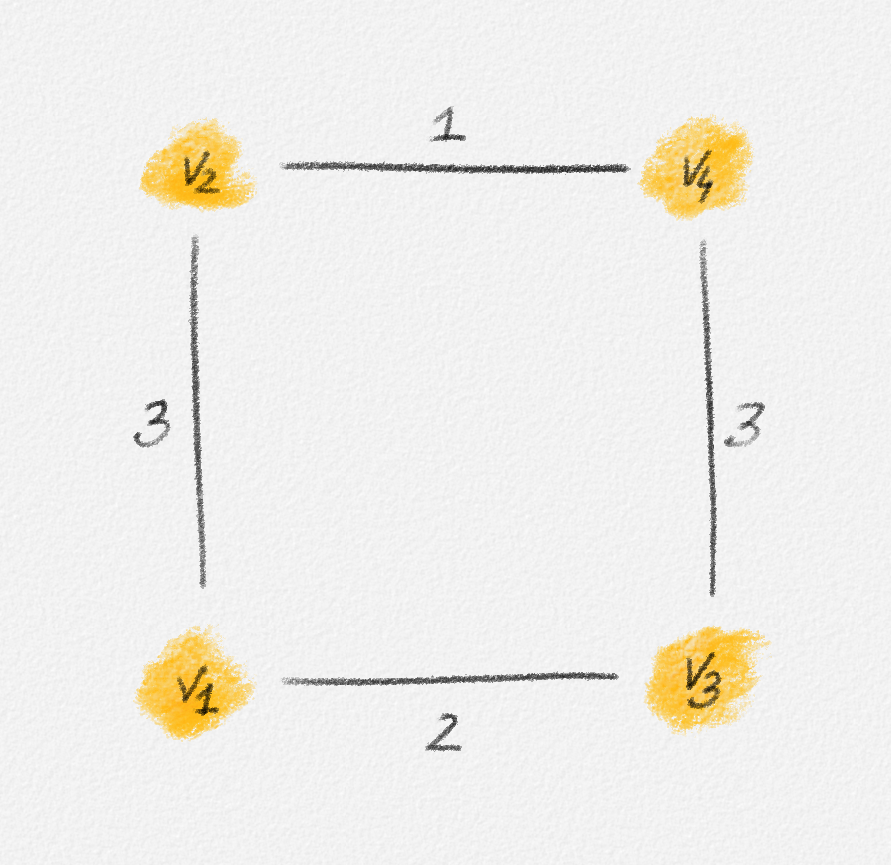
Figure 2.17: Since the edges \((v_1, v_2)\) and \((v_3, v_4)\) have the same weight, any fractional solution of (2.17) with \(x_{12} = \alpha\), \(x_{34} = 1 - \alpha\), and \(x_{13} = x_{24} = 1\) is an optimal solution.

It is easily verified that, at least in this example, any optimal fractional solution has the same objective function value as an optimal integral solution, that is, the optimal solution of the ILP is also an optimal solution of its relaxation. As we will show in Section 4.4, this is always the case. (We postpone the proof because we do not have the tools to construct the proof yet.) Moreover, it can be shown that if we use the Simplex Algorithm to find a solution of the LP relaxation of (2.16), the computed solution is always integral. The proof uses two facts that we do not prove here:

• Recall that the feasible region of an LP is a convex polytope in \(\mathbb{R}^n\). A geometric view of the Simplex Algorithm is that it moves between vertices of this polytope until it reaches a vertex that represents an optimal solution.

• Every vertex of the polytope defined by the LP relaxation of (2.16) represents an integral solution.

How useful is it that the LP relaxation of (2.16) has an integral optimal solution, given that this LP has exponentially many constraints? Doesn't it still take exponential time to solve this LP even using an algorithm whose running time is polynomial in the number of constraints? As mentioned in Section 2.4, the Ellipsoid Algorithm can solve every LP in polynomial time for which we can provide a polynomial-time separation oracle. The constraints in the LP relaxation of (2.16) are derived from the given edge-weighted graph \((G,w)\), whose representation uses only polynomial space, and it turns out that an appropriate separation oracle for the MST problem can be implemented in polynomial time based on this graph representation, without explicitly inspecting all constraints. Thus, the LP relaxation of (2.16) can in fact be solved in polynomial time. Still, sticking to Kruskal's or Prim's algorithm seems to be the much easier and generally more efficient approach for computing MSTs. The purpose of the Section 2.3 and of this section was simply to illustrate linear programming using a more elaborate example and to introduce integer linear programming and LP relaxations.