7.6.1. An Even Faster Implementation of the Hungarian Algorithm*

The Hungarian Algorithm does not use the fact that the input graph is complete in any way. We even used an incomplete graph to illustrate the algorithm in Figure 7.14. Completeness only guarantees that the graph has a perfect matching, provided that \(|U| = |W|\). If we run the algorithm on an incomplete graph, it may fail because there may not exist a perfect matching even if \(|U| = |W|\). Figure 7.15 shows an example. If we want to run the Hungarian algorithm on arbitrary bipartite graphs, we need to include an appropriate test whether there even exists a perfect matching. We will discuss this test in Section 7.6.1.4.

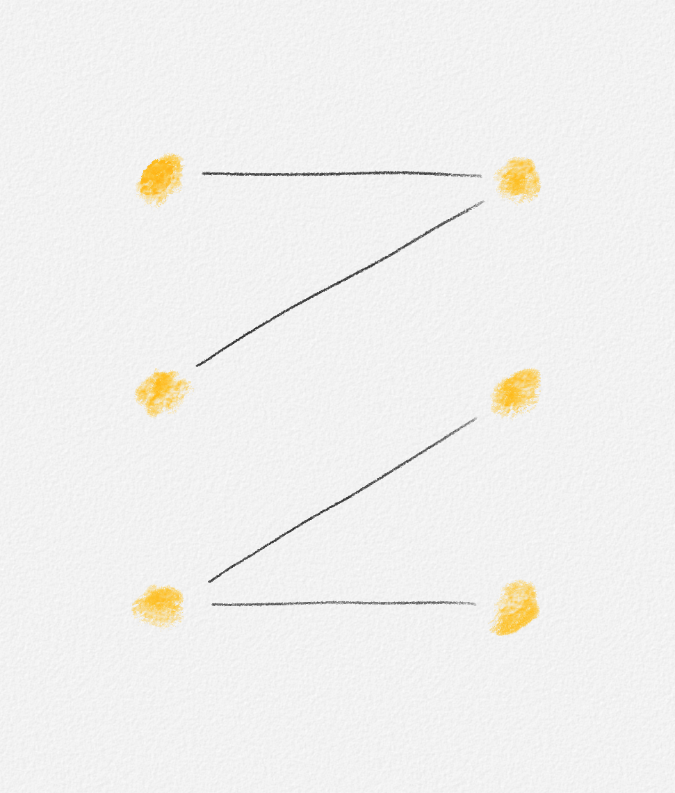
Figure 7.15: A trivial example of a bipartite graph where \(|U| = |W|\) but there is no perfect matching.

The \(O\bigl(n^3\bigr)\) running time of the Hungarian Algorithm in its current form is the result of its running for \(n\) phases, each of which takes \(O\bigl(n^2\bigr)\) time. To reduce the running time of the algorithm to \(O\bigl(n^2\lg n + nm\bigr)\), we show how to reduce the cost per phase to \(O(n \lg n + m)\).

We will show that the initialization of each phase already takes \(O(n + m)\) time. The looser \(O\bigl(n^2\bigr)\) bound on its cost that we obtained before was the result of us not being careful enough in the analysis.¹

The more challenging part is to reduce the cost of all up to \(2n\) iterations in each phase to \(O(n \lg n + m)\). To do this, we show that the last iteration in each phase can be implemented in \(O(n)\) time, and any other iteration can be implemented in \(O(\lg n + \deg(u))\) time, where \(u\) and \(w\) are the vertices moved from \(\bar X\) and \(\bar Y\) to \(X\) and \(Y\) in this iteration. Note that this means that the average cost per iteration is sublinear in \(n\) if \(G\) is sparse. This is something we can achieve only by using appropriate data structures, a priority queue in this case. The initialization of each phase needs to be modified to initialize the priority queue, but this does not increase its cost above \(O(n + m)\).

In Section 7.6.1.1, we start by discussing the data structures we maintain. Then, in Section 7.6.1.2, we discuss the initialization phase and its cost. In Section 7.6.1.3, we show how each iteration, except the last, can be implemented in \(O(\lg n + \deg(u))\) time, and that the last iteration can be implemented in \(O(n)\) time. Section 7.6.1.4 discusses how we detect that no perfect matching exists, so we can abort the algorithm in this case. Finally, Section 7.6.1.5 puts all the pieces together to obtain the fastest version of the Hungarian algorithm we discuss in these notes.