5. Maximum Flows

Consider a network of computers. Each network link has a certain bandwidth; some are Gigabit Ethernet links, some may be good old-fashioned 10M links, some may be wireless links. The goal is to design a cooperative data transfer protocol that can send large files between locations as quickly as possible. Clearly, it would be fastest to use a route consisting of only Gigabit Ethernet links when sending lots of data from point A to point B. If there are two edge-disjoint routes consisting of only Gigabit Ethernet links, then the transmission time can be halved by sending half of the file along one route and the other half along the other route. Even though the 10M links by themselves are slow, adding a route of 10M links to the mix nevertheless reduces the load on the two Gigabit routes and reduces the transmission time a little more. Now, everybody likes the fast Gigabit Ethernet links and tries to utilize them to send their data, so it may be the case that only a fraction of the full bandwidth of these links is available for use by the file transfer protocol.

Abstractly, the network can be described as a directed graph \(G = (V, E)\) whose edges have non-negative capacities (bandwidths) \(u_e\). The goal is to determine how much flow (data) can be sent from a source \(s \in V\) to a sink (destination) \(t \in V\) and how much of it is sent along each edge \(e \in E\). The flow sent along edge \(e\) is denoted by \(f_e\). This flow has to satisfy two natural constraints (see Figure 5.1):

Capacity constraints: The flow sent along an edge \(e\) cannot be negative and cannot exceed the edge's capacity:

\[0 \le f_e \le u_e\quad \forall e \in E.\]

Flow conservation: No node other than the source or sink generates or absorbs any flow, that is, the amount of flow entering this node must equal the amount of flow leaving this node:

\[\sum_{(x,y) \in E} f_{x,y} = \sum_{(y,z) \in E} f_{y,z}\quad \forall y \in V \setminus \{ s, t \}.\]

A flow function \(f\) that satisfies these two conditions is called a feasible \(\boldsymbol{st}\)-flow.

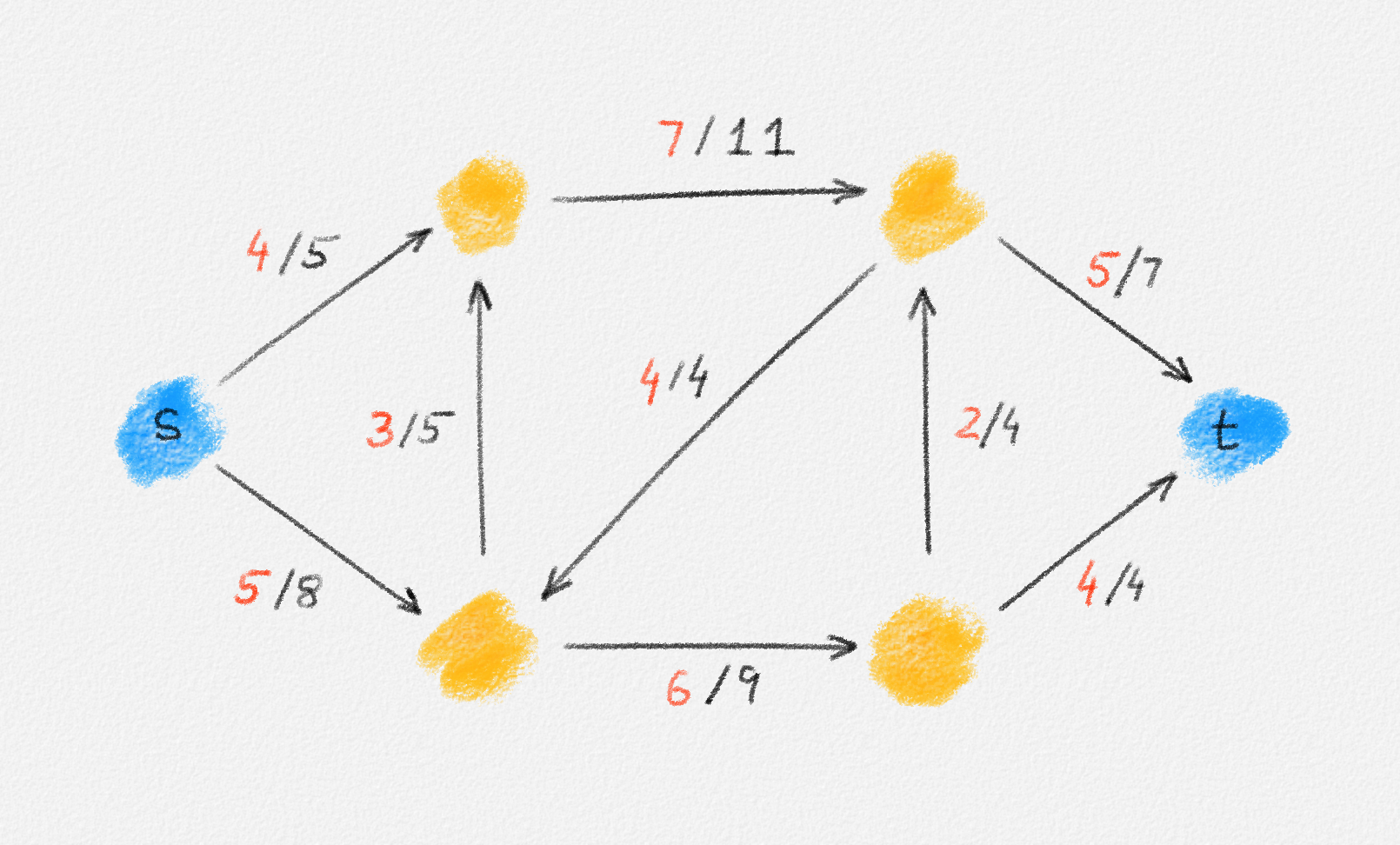
Figure 5.1: A network \(G\) and a feasible \(st\)-flow \(f\). Edge capacities are shown in black. The flow across every edge is shown in red.

The total amount of flow sent from \(s\) to \(t\) is the net out-flow of \(s\),

\[\sum_{(s,z) \in E} f_{s,z} - \sum_{(x,s) \in E} f_{x,s},\]

which must equal the net in-flow of \(t\),

\[\sum_{(x,t) \in E} f_{x,t} - \sum_{(t,z) \in E} f_{t,z},\]

as a result of flow conservation. It will be convenient to have a notation for the net flow produced by each node:

\[F_y = \sum_{(y,z) \in E} f_{y,z} - \sum_{(x,y) \in E} f_{x,y}.\]

Then flow conservation states that

\[\begin{aligned} F_s &= -F_t && \text{and}\\ F_x &= 0 && \forall x \notin \{s, t\}. \end{aligned}\]

A feasible \(st\)-flow \(f\) is a maximum \(\boldsymbol{st}\)-flow if \(F_s \ge F'_s\) for every feasible \(st\)-flow \(f'\).

This gives the following graph problem, expressed in the language of linear programming:

Maximum flow problem: Given a directed graph \(G = (V, E)\), an assignment of capacities \(u : E \rightarrow \mathbb{R}^+\) to its edges, and an ordered pair of vertices \((s,t)\), compute a maximum \(st\)-flow \(f\), that is, an assignment \(f : E \rightarrow \mathbb{R}^+\) of flows to the edges of \(G\) such that \(F_s\) is maximized and

\[\begin{aligned} 0 \le f_e &\le u_e && \forall e \in E\\ F_x &= 0 && \forall x \in V \setminus \{s, t\}. \end{aligned}\]

Note that we use the term "flow" to refer to the whole function \(f\) and to refer to the "flow along an edge \(e\)", the value \(f_e\). The meaning will be clear from context.

Given the expression of the maximum flow problem as a linear program, it can be solved using the Simplex Algorithm. This approach, but using a more efficient implementation that operates directly on the graph instead of explicitly translating the graph into a set of linear constraints, is known as the Network Simplex algorithm and is one of the fastest ways to compute maximum flows, and also minimum-cost flows discussed in Chapter 6, in practice. The focus in this chapter is on algorithms that solve the maximum flow problem directly, without using linear programming.

Throughout this chapter and the next, we will refer to an absent edge as an edge of capacity \(0\): Such an edge clearly carries no flow. This allows us to simplify notation, for example, by defining

\[F_x = \sum_{y \in V} \bigl(f_{x,y} - f_{y,x}\bigr),\]

which is equivalent to the definition given above.

The discussion of maximum flow algorithms in this chapter is organized as follows:

• In Section 5.1, we discuss augmenting path algorithms, which are algorithms that maintain a feasible flow and repeatedly send more flow along paths from \(s\) to \(t\). These algorithms are called augmenting path algorithms because every time we send more flow from \(s\) to \(t\) along such a path, we augment the flow.

• In Section 5.2, we discuss preflow-push algorithms. These algorithms do not maintain a feasible flow! Instead, they start from the observation that the most flow we could possibly send from \(s\) to \(t\) is the total capacity of all out-edges of \(s\). So these algorithms optimistically send \(u_{s,y}\) units of flow along each such edge \((s, y)\). This creates an excess of in-flow at the out-neighbours of \(s\). This excess flow is then moved onwards along the out-edges of these out-neighbours until some of this flow reaches \(t\). Once we cannot move more flow to \(t\) using this strategy, the remaining excess flow is moved back to \(s\): We were too optimistic with the initial amount of flow we moved along the out-edges of \(s\).

  At any stage during the execution of a preflow-push algorithm, the flow function \(f\) satisfies the capacity constraints but may violate flow conservation. We call such a flow function a preflow. The operation we use to move flow from some vertex with excess in-flow to one of its out-neighbours is called a push operation. Hence the name of these algorithms.

• The final question we address, in Section 5.3, is under which conditions there exists an integral maximum \(st\)-flow in the network \(G\) and whether augmenting path and preflow-push algorithms find such a flow if it exists. This will be important, for example, when discussing maximum matchings in Section 7.3.