5.1. Augmenting Path Algorithms

Two of the oldest maximum flow algorithms are due to Ford and Fulkerson and Karp and Edmonds. These algorithms are known as augmenting path algorithms because they start with the trivial \(st\)-flow \(f_e = 0\ \forall e \in E\), which is clearly feasible, and then repeatedly find paths from \(s\) to \(t\) along which more flow can be pushed from \(s\) to \(t\) while maintaining the feasibility of the flow. These algorithms are based on two key observations:

• Assume that \(f\) is a feasible \(st\)-flow in \(G\) and that there exists a path from \(s\) to \(t\) such that every edge \(e \in P\) satisfies \(u_e - f_e > 0\). In other words, none of the edges in \(P\) is used to its full capacity. Then \(P\) is an augmenting path in the sense that we can send additional flow along this path:

  If \(\delta = \min \{ u_e - f_e \mid e \in P \}\), then the \(st\)-flow \(f'\) defined as

  \[f'_e = \begin{cases} f_e + \delta & \text{if } e \in P\\ f_e & \text{otherwise} \end{cases}\]

  is feasible and satisfies \(F'_s > F_s\). See Figure 5.2.

  ---

  

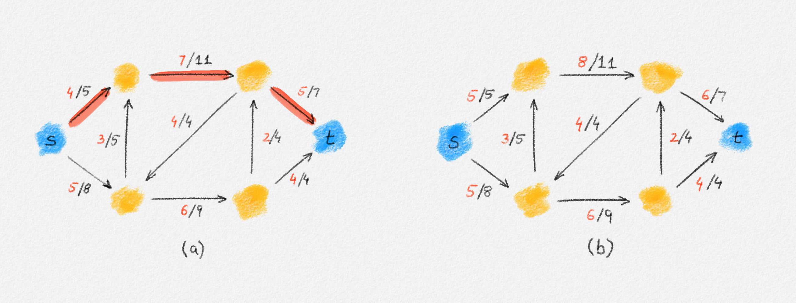
  Figure 5.2: (a) An augmenting path for the flow in Figure 5.1 that uses only edges in \(G\). (b) The flow obtained by sending one unit of flow along the path in (a).

  ---

• An augmenting path can also push flow from \(y\) to \(x\) (!) along an edge \((x,y)\) if \(f_{x,y} > 0\). Indeed, this amounts to sending some of the flow currently flowing from \(x\) to \(y\) back to \(x\), that is, reducing the flow \(f_{x,y}\) along the edge \((x,y)\) and diverting the sent-back flow to a different out-neighbour of \(x\). See Figure 5.3.

  ---

  

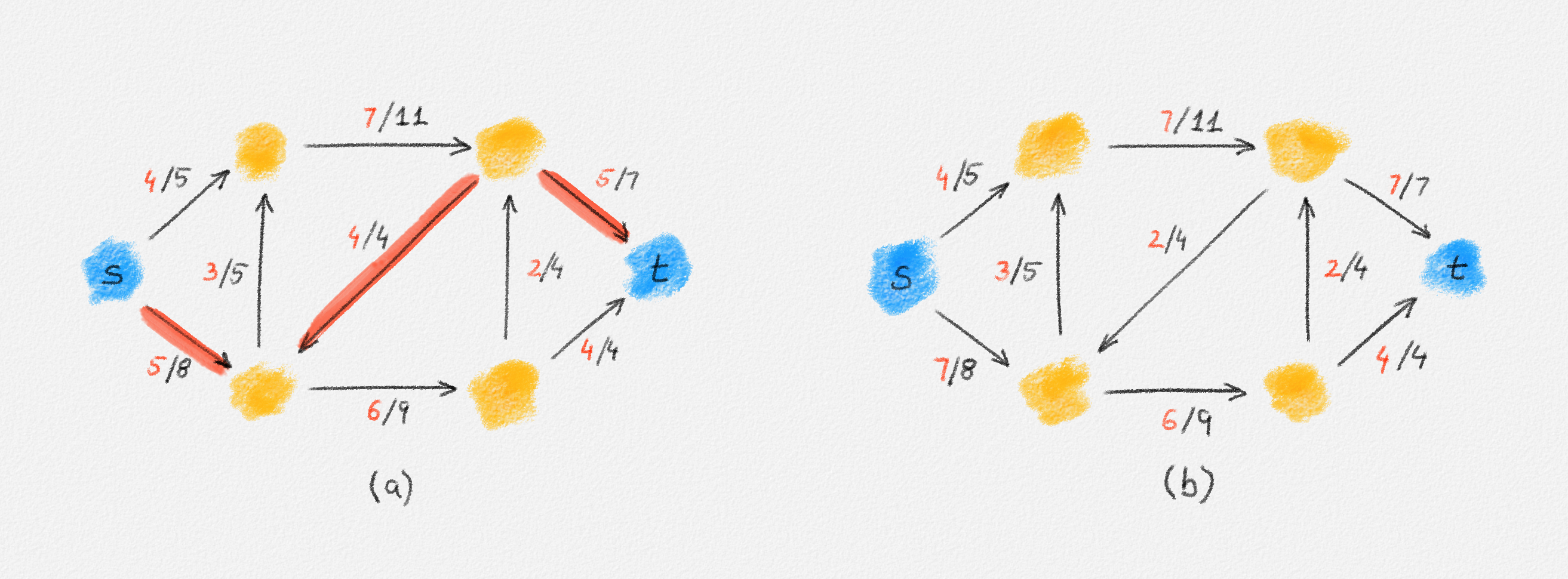
  Figure 5.3: (a) An augmenting path for the flow in Figure 5.1 that uses an edge of \(G\) in reverse. (b) The flow obtained by sending two units of flow along the path in (a).

  ---

The set of edges along which we can try to move more flow from \(s\) to \(t\) is the edge set \(E^f\) of the residual network \(G^f = \bigl(V, E^f\bigr)\) corresponding to \(f\):

The residual network of a graph \(G = (V, E)\) is the network \(G^f = \bigl(V, E^f\bigr)\), where

\[E^f = \{(x,y) \in E \mid f_{x,y} < u_e\} \cup \{(y, x) \mid (x, y) \in E \text{ and } f_{x,y} > 0\}.\]

The residual capacity of an edge \((x, y) \in E^f\) is

\[u^f_{x,y} = f_{y,x} + u_{x,y} - f_{x,y}.\]

This is illustrated in Figure 5.4.

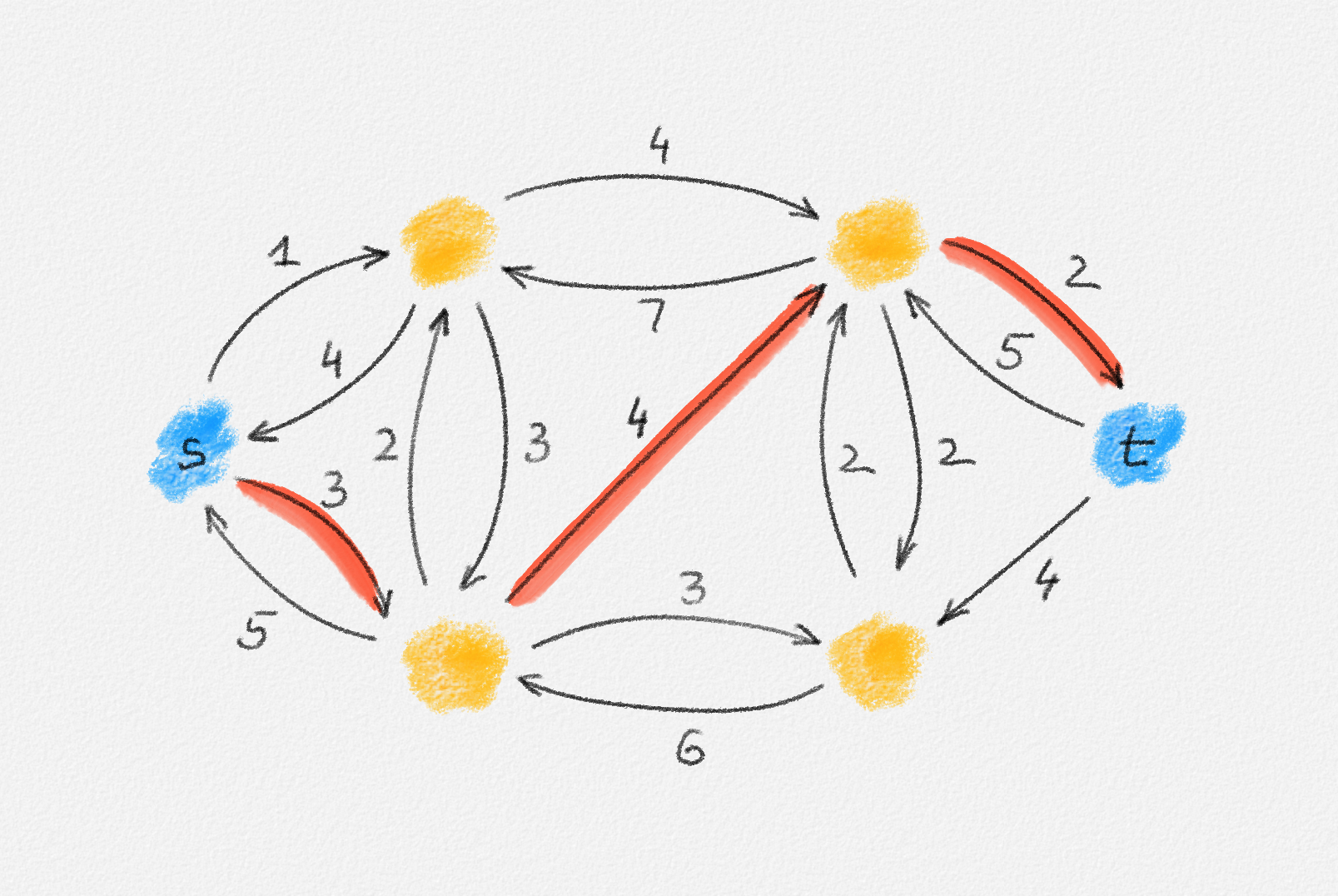
Figure 5.4: The residual network \(G^f\) corresponding to the flow in Figure 5.1. The augmenting path in Figure 5.3(a) is a directed path in \(G^f\) (red).

If \((x, y) \in E^f\) because \(f_{x,y} < u_{x,y}\), then this means that the edge \((x, y) \in E\) is not used to its full capacity and we can move up to \(u_{x,y} - f_{x,y}\) units of flow along this edge in an attempt to increase the flow from \(s\) to \(t\).

If \((x, y) \in E^f\) because \(f_{y,x} > 0\), then this means that we can move up to \(f_{y,x}\) units of flow from \(y\) back to \(x\).

It is possible that the network \(G\) contains both edges \((x, y)\) and \((y, x)\). In this case, we can move up to \(u_{x,y} - f_{x,y}\) additional units of flow from \(x\) to \(y\) along the edge \((x, y)\), and we can move up to \(f_{y,x}\) units of flow from \(x\) to \(y\) by pushing flow back along the edge \((y, x)\). This is captured by the residual capacity of the edge \((x, y)\) in \(G^f\), which is the sum of these two quantities.

With this definition of the residual network in place, we can define an augmenting path formally:

Given a feasible \(st\)-flow \(f\) in \(G\), an augmenting path \(P\) is a path from \(s\) to \(t\) in the residual network \(G^f\).

Every augmenting path algorithm starts with the trivial flow \(f_e = 0\) for all \(e \in G\) and then repeatedly finds augmenting paths along which to move more flow from \(s\) to \(t\) until there are no augmenting paths left. This is the strategy of the Ford-Fulkerson algorithm, which we discuss in Section 5.1.1. As we will see, the Ford-Fulkerson algorithm may not terminate on certain inputs. However, we will prove that it computes a maximum \(st\)-flow if it does terminate. Since all other augmenting path algorithms are variations of the Ford-Fulkerson algorithm, their correctness follows from that of the Ford-Fulkerson algorithm.

The remainder of this section is organized as follows:

• In Section 5.1.1, we discuss the Ford-Fulkerson algorithm.

• The first variation of the Ford-Fulkerson algorithm we discuss, in Section 5.1.2, is the Edmonds-Karp algorithm. Its only difference from the basic Ford-Fulkerson algorithm is that it always finds a shortest augmenting path along which to send more flow from \(s\) to \(t\). We will show that this choice of an augmenting path guarentees that the algorithm terminates, in \(O\bigl(nm^2\bigr)\) time, where \(n\) is the number of vertices and \(m\) is the number of edges in the network.

• Dinitz's algorithm is a further improvement over the Edmonds-Karp algorithm, with running time \(O\bigl(n^2m\bigr)\). We discuss this algorithm in Section 5.1.3. For dense graphs—ones where \(m = \Omega\bigl(n^2\bigr)\)—this is faster than the Edmonds-Karp algorithm by a factor of \(\Theta(n)\). One way to summarize the main idea of Dinitz's algorithm is that it finds many augmenting paths and sends flow along all of these paths simultaneously. Thus, it approaches a maximum flow faster.