2.3.3. An ILP Formulation of Polynomial Size*

In an attempt to reduce the difficulty of solving the MST problem formulated as an ILP, let us aim to develop an ILP formulation of the MST problem with only a polynomial number of constraints. The following, substantially less intuitive ILP formulation has only \(O\bigl(nm^2\bigr)\) constraints.

The tree structure of \(T\) is enforced using additional variables \(y_e^v \in \{0, 1\}\) and constraints on these variables. Fix an arbitrary vertex \(s \in V\). Then \(y_e^v = 1\) if and only if \(e\) belongs to the path from \(s\) to \(v\) in \(T\). Now the following observations capture that \(T\) is a tree:

• If the edge \((u,v)\) is in \(T\), then it belongs to the path from \(s\) to \(v\) or to the path from \(s\) to \(u\) but not both. If \((u,v) \notin T\), then it is not on any path. This can be expressed using the following constraint:

  \[y_{u,v}^u + y_{u,v}^v = x_{u,v} \quad \forall (u,v) \in E.\]

• Every vertex \(v \ne s\) has exactly one incident edge \((u,v)\) that belongs to the path from \(s\) to \(v\):

  \[\sum_{(u,v) \in E} y_{u,v}^v = 1 \quad \forall v \ne s.\]

  For \(v = s\), none of the edges incident to \(s\) belongs to the path from \(s\) to \(s\):

  \[\sum_{(s,v) \in E} y_{s,v}^s = 0.\]

• If the edge \((u,v)\) belongs to the path from \(s\) to \(v\) and the edge \((v,w)\) belongs to the path from \(s\) to some vertex \(z\), then the edge \((u,v)\) also belongs to the path from \(s\) to \(z\):

  \[y_{u,v}^z \ge y_{u,v}^v + y_{v,w}^z - 1 \quad \forall z \in V, (u,v) \in E, (v,w) \in E.\]

This gives the following ILP formulation of the MST problem:

\[\begin{gathered} \text{Minimize } \sum_{e \in E} w_e x_e\\ \begin{aligned} \text{s.t. } \phantom{y_{u,v}^u + y_{u,v}^v} \llap{\displaystyle\sum_{e \in E} x_e} &= n - 1\\ y_{u,v}^u + y_{u,v}^v &= x_{u,v} && \forall (u,v) \in E\\ \sum_{(s,v) \in E} y_{s,v}^s &= 0\\ \sum_{(u,v) \in E} y_{u,v}^v &= 1 && \forall v \ne s\\ y_{u,v}^z &\ge y_{u,v}^v + y_{v,w}^z - 1 && \forall z \in V, (u,v) \in E, (v,w) \in E\\ x_e &\in \{0, 1\} && \forall e \in E\\ y_e^v &\in \{0, 1\} && \forall v \in V, e \in E. \end{aligned} \end{gathered}\tag{2.11}\]

This ILP does indeed have polynomial size because, apart form the first three constraints, there are \(n - 1\) copies of the fourth constraint, one per vertex \(v \ne s\); no more than \(nm^2\) copies of the fifth constraint, at most one per vertex \(z \in V\) and per pair of edges \((u,v)\) and \((v, w)\) in \(E\); \(m\) copies of the sixth constraint, one per edge; and \(nm\) copies of the last constraint, one per pair \((v, e)\), where \(v\) is a vertex and \(e\) is an edge.

While the correctness of (2.9) and (2.10) should be obvious, the correctness of (2.11) requires some effort to prove. The next lemma and corollary show that it is indeed a correct formulation of the MST problem.

Lemma 2.4: For any undirected edge-weighted graph \((G,w)\), \(\bigl(\hat x, \hat y\bigr)\) is a feasible solution of (2.11) if and only if the subgraph \(T = (V, E')\) of \(G\) with \(E' = \bigl\{ e \in E \mid \hat x_e = 1 \bigr\}\) is a spanning tree of \(G\).

Proof: The first constraint of (2.11) ensures that every feasible solution \(\bigl(\hat x, \hat y\bigr)\) satisfies \(\sum_{e \in E} \hat x_e = n - 1\). Since an \(n\)-vertex graph is a tree if and only if it has \(n - 1\) edges and is acyclic, it therefore suffices to prove that \(\bigl(\hat x, \hat y\bigr)\) is a feasible solution of (2.11) if and only if \(T\) contains no cycle.

So assume first, for the sake of contradiction, that \(\bigl(\hat x, \hat y\bigr)\) is a feasible solution and that \(T\) contains a cycle \(C = \langle v_0, v_1, \ldots, v_k \rangle\). Then \(\hat x_{v_{i-1},v_i} = 1\) for all \(1 \le i \le k\). Since \(\hat y_{v_{i-1},v_i}^{v_{i-1}} + \hat y_{v_{i-1},v_i}^{v_i} = \hat x_{v_{i-1},v_i}\), this implies that either \(\hat y_{v_{i-1},v_i}^{v_{i-1}} = 1\) or \(\hat y_{v_{i-1},v_i}^{v_i} = 1\) for all \(1 \le i \le k\). If there exists a vertex \(v_i\) such that \(\hat y_{v_{i-1},v_i}^{v_i} = 1\) and \(\hat y_{v_i,v_{i+1}}^{v_i} = 1\), then \(\sum_{(u,v_i) \in E} \hat y_{u,v_i}^{v_i} > 1\), a contradiction. Thus, we can assume w.l.o.g. that \(\hat y_{v_{i-1},v_i}^{v_i} = 1\) and \(\hat y_{v_{i-1},v_i}^{v_{i-1}} = 0\) for all \(1 \le i \le k\). In particular, \(y_{v_0,v_1}^{v_0} = 0\).

Now observe that \(\hat y_{v_{i-1},v_i}^{v_k} = 1\) for all \(1 \le i \le k\). The proof is by induction on \(j = k - i\). For the base case, \(i = k\), we just observed that \(\hat y_{v_{k-1},v_k}^{v_k} = 1\). For the inductive step, \(i < k\), observe that, by the inductive hypothesis, \(\hat y_{v_i,v_{i+1}}^{v_k} = 1\). Since \(\hat y_{v_{i-1},v_i}^{v_i} = 1\), \(\hat y_{v_{i-1},v_i}^{v_k} \ge \hat y_{v_{i-1},v_i}^{v_i} + y_{v_i,v_{i+1}}^{v_k} - 1\), and \(\hat y_{v_{i-1},v_i}^{v_k} \in \{0,1\}\), we have \(\hat y_{v_{i-1},v_i}^{v_k} = 1\).

Since \(\hat y_{v_{i-1},v_i}^{v_k} = 1\) for all \(1 \le i \le k\), we have in particular that \(\hat y_{v_0,v_1}^{v_k} = 1\). Since \(C\) is a cycle, we have \(v_k = v_0\), that is, \(\hat y_{v_0,v_1}^{v_0} = 1\), a contradiction because we observed above that \(\hat y_{v_0, v_1}^{v_0} = 0\). Thus, \(T\) cannot contain any cycles if \(\bigl(\hat x, \hat y\bigr)\) is a feasible solution of (2.11).

Now assume that \(T\) is a tree and define \(\hat x_e = 1\) if and only if \(e \in T\) and \(\hat y_e^v = 1\) if and only if the edge \(e\) is on the path from \(s\) to \(v\) in \(T\). Since \(T\) has \(n - 1\) edges, we have \(\sum_{e \in E} \hat x_e = n - 1\).

If we consider an edge \((u, v) \in T\), then let \(T_u\) and \(T_v\) be the two subtrees of \(T\) obtained by removing the edge \((u, v)\). See Figure 2.11.

Figure 2.11: The two subtrees \(T_u\) and \(T_v\) of \(T\) obtained by removing the edge \((u, v)\).

If \(s \in T_u\), then \((u, v)\) belongs to the path from \(s\) to \(v\) but not to the path from \(s\) to \(u\). If \(s \in T_v\), then \((u, v)\) belongs to the path from \(s\) to \(u\) but not to the path from \(s\) to \(v\). In both cases, \(\hat y_{u,v}^u + \hat y_{u,v}^v = 1 = \hat x_{u,v}\). If \((u, v) \notin T\), then \(\hat y_{u,v}^u + \hat y_{u,v}^v = 0 = \hat x_{u,v}\).

Since no edge in \(T\) belongs to the path from \(s\) to \(s\), we have \(\sum_{(s, v) \in E} \hat y_{s,v}^s = 0\). For \(v \ne s\), let \(u_1, \ldots, u_d\) be the neighbours of \(v\) in \(T\). Removing the edges \((u_1,v), \ldots, (u_d,v)\) breaks \(T\) into \(d + 1\) connected components. One contains only \(v\); the others are subtrees \(T_{u_1}, \ldots, T_{u_d}\) containing the vertices \(u_1, \ldots, u_d\), respectively. There exists exactly one such tree \(T_{u_i}\) that contains \(s\). In this case, the edge \((u_i,v)\) belongs to the path from \(s\) to \(v\) and the other edges \((u_j,v)\) with \(j \ne i\) do not. Thus, \(\sum_{j=1}^d \hat y_{u_j,v}^v = \sum_{(u,v) \in E} \hat y_{u,v}^v = 1\). See Figure 2.12.

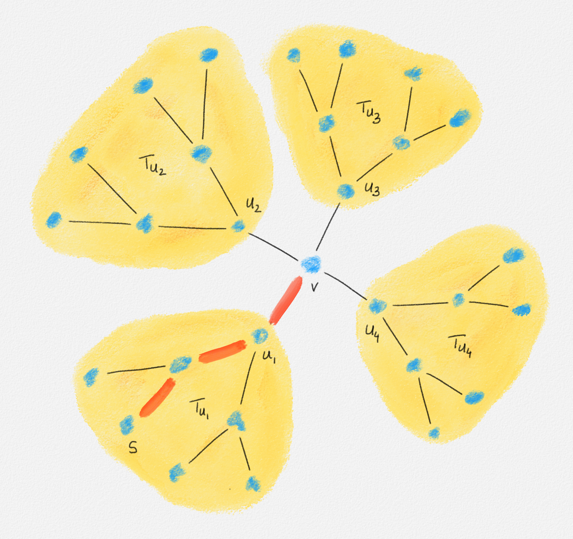
Figure 2.12: Exactly one of the edges incident to a vertex \(v \ne s\) belongs to the path from \(s\) to \(v\).

Finally, consider any two edges \((u,v), (v,w) \in E\) sharing an endpoint and any vertex \(z \in V\). If \((u,v)\) does not belong to the path from \(s\) to \(v\), then \(\hat y_{u,v}^v = 0\). If \((v,w)\) does not belong to the path from \(s\) to \(z\), then \(\hat y_{v,w}^z = 0\). In either case, \(\hat y_{u,v}^v + \hat y_{v,w}^z - 1 \le 0\). Thus, \(\hat y_{u,v}^z \ge 0 \ge \hat y_{u,v}^v + \hat y_{v,w}^z - 1\).

If \((u,v)\) belongs to the path from \(s\) to \(v\), and \((u,v)\) and \((v,w)\) belong to the path from \(s\) to \(z\), then \(\hat y_{u,v}^v = \hat y_{v,w}^z = 1\) and \(\hat y_{u,v}^z = 1 = \hat y_{u,v}^v + \hat y_{v,w}^z - 1\).

If \((u,v)\) belongs to the path from \(s\) to \(v\), \((v,w)\) belongs to the path from \(s\) to \(z\), and \((u,v)\) does not belong to the path from \(s\) to \(z\), then let \(P_1\) be the path from \(s\) to \(v\) in \(T\), and let \(P_2\) be the path from \(s\) to \(z\) in \(T\). Since the edge \((v,w)\) belongs to \(P_2\), so does the vertex \(v\). The subpath \(P_2'\) of \(P_2\) from \(s\) to \(v\) does not contain \((u,v)\) because \(P_2\) does not contain \((u,v)\). Thus, \(T\) contains two paths from \(s\) to \(v\), a contradiction because \(T\) is a tree. Therefore, this is not possible. In other words, \(\hat y_{u,v}^v = 1\) and \(\hat y_{v,w}^z = 1\) implies that \(\hat y_{u,v}^z = 1 = \hat y_{u,v}^v + \hat y_{v,w}^z - 1\). See Figure 2.13.

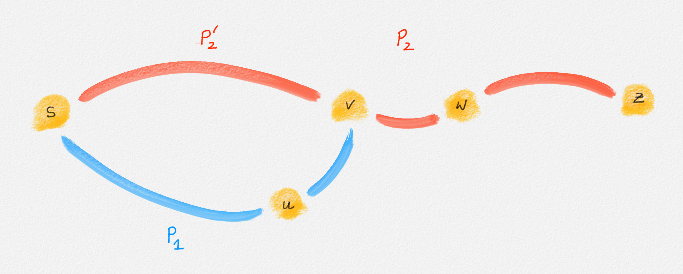
Figure 2.13: If \((u, v)\) belongs to the path from \(s\) to \(v\) and \((v, w)\) belongs to the path from \(s\) to \(z\) but \((u, v)\) does not, then \(T\) cannot be a tree.

This shows that the solution \(\bigl(\hat x, \hat y\bigr)\) corresponding to \(T\) is a feasible solution of (2.11). ▨

Since every feasible solution \(\bigl(\hat x, \hat y\bigr)\) of (2.11) defines a spanning tree of \(G\) and vice versa, we have:

Corollary 2.5: For any undirected edge-weighted graph \((G,w)\), \(\bigl(\hat x, \hat y\bigr)\) is an optimal solution of (2.11) if and only if the subgraph \(T = (V, E')\) of \(G\) with \(E' = \bigl\{ e \in E \mid \hat x_e = 1 \bigr\}\) is an MST of \((G,w)\).

The ILP (2.11) has only a polynomial number of constraints, while (2.9) and (2.10) have an exponential number of constraints. As we discuss next, this does not make (2.11) any easier to solve. The key to an efficient solution of the minimum spanning tree problem is to express it as a linear program, without requiring that the variables have integer values. It turns out that this is much easier to do for a slightly modified version of (2.9) than for any of the three ILPs (2.9), (2.10), and (2.11).