Mini-Project: Fibonacci Numbers
Let us look at the natural definition of Fibonacci numbers again:
fib :: Integer -> Integer
fib 0 = 0
fib 1 = 1
fib n = fib (n - 1) + fib (n - 2)
We already observed that this implementation is inefficient because it
calculates the \(n\)th Fibonacci number as the sum of a bunch of ones and zeroes.
Now that we know about tail recursion, we also observe that it uses a lot of
stack space (not all that much at any given point in time, but it creates and
destroys lots of stack frames) because neither fib (n - 1) nor fib (n - 2)
is in tail position in the third equation—we add their results together to
obtain the result of the current invocation fib n.
Our goal is to turn fib into a tail-recursive function that is essentially a
loop, and we want to reduce the number of iterations of this loop from
\(F_n\) to \(n\). This will give us a nice performance improvement.
I know I should make you do this in Haskell directly, but whenever we use tail recursion, we're looking for a pattern that's essentially a loop. Looking for this pattern in a language that actually has loops can be helpful. We use Python again.
As a starting point, let's write our Fibonacci function in Python:
def fib(n):
    if n == 0:
        return 0
    elif n == 1:
        return 1
    else:
        return fib(n - 1) + fib(n - 2)
If you've taken CSCI 3110 already, you have learned about dynamic programming.
The idea is to build a table that remembers values you've computed before so you
don't need to compute them from scratch again when you need them a second, third
or 1,000,001st time. For computing Fibonacci numbers, this approach is rather
effective because to compute \(F_n\), we only need to compute \(n\) other Fibonacci
numbers: \(F_0, \ldots, F_{n-1}\). Our strategy therefore is to keep a table where
we store the Fibonacci numbers we have already computed. Whenever we need to
know the value of a Fibonacci number, we first check whether we have already
computed it. In this case, we simply look it up in our table. Otherwise, we have
no choice but to compute it from scratch, but even that recursive computation
can utilize our table to avoid computing Fibonacci numbers again that we have
already computed. To make this work, we need an object that holds our table of
already computed Fibonacci numbers. The function that computes Fibonacci numbers
needs to be a method of this object because it needs access to the table. Our
main Fibonacci function creates an object capable of storing \(F_0\) up to \(F_n\)
and then calls the fib method of this object to compute \(F_n\):
def fib(n):
    f = Fib(n)
    return f.fib(n)
The constructor of our Fib class takes the index of the Fibonacci number to be
computed as argument, to create an array big enough to hold the first \(n + 1\)
Fibonacci numbers. Initially, each table entry is None because we haven't
computed any Fibonacci numbers yet:
def fib(n):
    f = Fib(n)
    return f.fib(n)

class Fib:

    def __init__(self, n):
        self.fibs = [None] * (n + 1)
Now for the core of the program: Fib.fib. This function implements exactly
the same logic as our original definition of fib, only it uses the table
Fib.fibs to speed up its computation:
class Fib:

    def __init__(self, n):
        self.fibs = [None] * (n + 1)

    def fib(self, n):
        if self.fibs[n] is None:
            if n == 0:
                self.fibs[n] = 0
            elif n == 1:
                self.fibs[n] = 1
            else:
                self.fibs[n] = self.fib(n - 1) + self.fib(n - 2)
        return self.fibs[n]
First it checks whether self.fibs[n] is not None. In that case, we have
already computed the \(n\)th Fibonacci number, and we simply return it.
Otherwise, we need to compute it. The body of the if-statement does this, in
exactly the same fashion as our original fib function, only it stores its
result in self.fibs[n] instead of returning it directly, so any subsequent
call to fib with argument n can simply look up the \(n\)th Fibonacci
number.
This is illustrated in the following figure, which shows the tree of recursive
calls made by the invocation fib(5). The arrows to and from the fibs table
show which recursive call stores some value fib(i) in the corresponding slot
of the fibs table and which recursive calls simply read their results from
the fibs table.
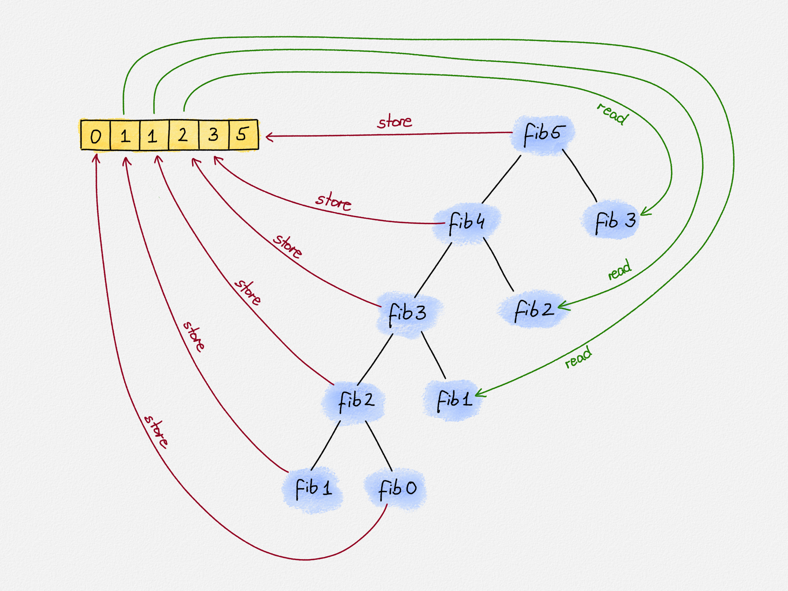
Illustration of dynamic programming for computing Fibonacci numbers
You can try this out. It computes large Fibonacci numbers quickly. Computing \(F_n\) takes \(O(n)\) time now. However, the code is not as space-efficient nor as elegant as it could be. It uses \(O(n)\) space for the table of Fibonacci numbers, but constant space is possible. Let's improve it.
The first improvement is a step in the right direction even though it does not substantially change the amount of space our code needs—we still build a table of the first \(n\) Fibonacci numbers:
def fib(n):
    fibs = [None] * (n + 1)

    for i in range(0, n + 1):
        if i == 0:
            fibs[i] = 0
        elif i == 1:
            fibs[i] = 1
        else:
            fibs[i] = fibs[i - 1] + fibs[i - 2]

    return fibs[n]
This code completely does away with recursive calls. It iteratively computes the
first \(n + 1\) Fibonacci numbers, again using exactly the standard formula for
Fibonacci numbers: fibs[0] = 0, fibs[1] = 1, and
fibs[i] = fibs[i - 1] + fibs[i - 2]. This works because we compute Fibonacci
numbers by increasing indices, so when it's time to compute fibs[i], we have
already computed fibs[i - 1] and fibs[i - 2]. We can simply look them up in
the table, add them together, and store the result in fibs[i].
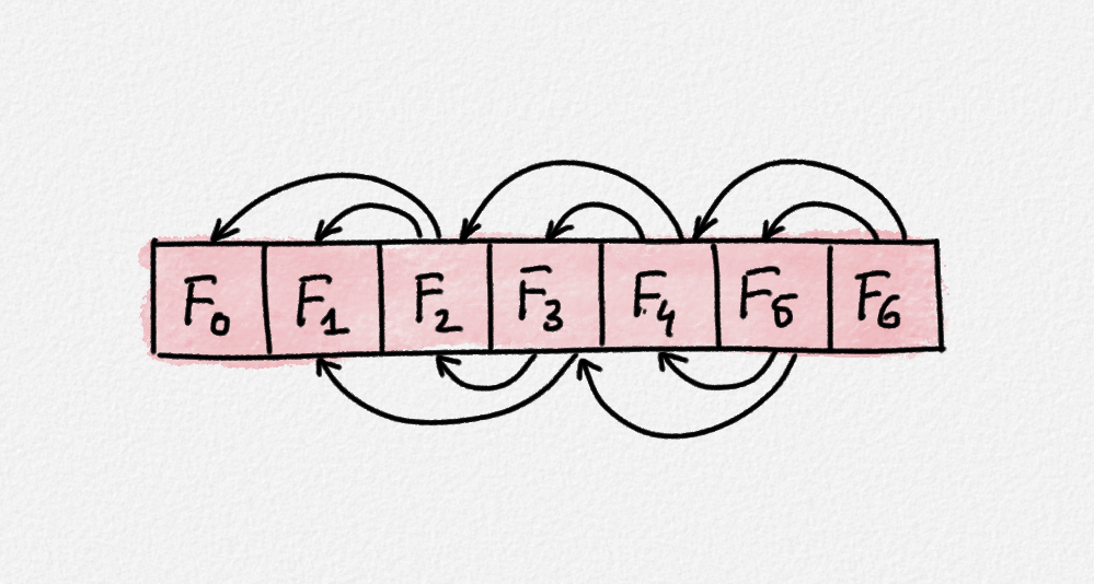
Dependencies between table entries in the Fibonacci function
Now let's come up with the final version of our Python function to compute
Fibonacci numbers. If you look a little closer, you'll notice that each
iteration of the for-loop relies only on the values computed in the previous two
iterations: To compute fibs[2], we need access to fibs[0] and fibs[1]. To
compute fibs[3], we need access to fibs[2] and fibs[1]. And so on. So
keeping the entire table of Fibonacci numbers is wasteful. We only need to
remember the two Fibonacci numbers computed in the current iteration and in the
previous iteration. To avoid strange hacks such as defining \(F_{-1} = 1\), let us
set up the computation so that at the beginning of the ith iteration of the
loop, we have variables f_i and f_i_plus_1 containing the ith and
(i+1)st Fibonacci numbers. To ensure this invariant holds in the first
iteration of the loop, when i = 0, we need to set f_i = 0 (\(F_0\)) and
f_i_plus_1 = 1 (\(F_1\)):
def fib(n):
    f_i = 0
    f_i_plus_1 = 1
If f_i holds the ith Fibonacci number and f_i_plus_1 holds the (i+1)st
Fibonacci number, then to ensure that the same invariant holds in the next
iteration, where i is increased by one, we need to replace f_i with
f_i_plus_1 and f_i_plus_1 with f_i + f_i_plus_1:
def fib(n):
    f_i = 0
    f_i_plus_1 = 1

    for i in range(0, n):
        f_i, f_i_plus_1 = f_i_plus_1, f_i + f_i_plus_1
After the last iteration, we have i = n. Thus, at the end of this iteration,
f_i stores \(F_n\). We can now return this value:
def fib(n):
    f_i = 0
    f_i_plus_1 = 1

    for i in range(0, n):
        f_i, f_i_plus_1 = f_i_plus_1, f_i + f_i_plus_1

    return f_i
Now back to Haskell. Let's translate our Python function into a tail-recursive
Haskell function. We use the same recipe as in the previous section: We
implement the loop as a recursive function. The arguments of this function are
the variables that change in the loop of our Python function, here the current
index i, f_i, and f_i_plus_1. i changes to i + 1. f_i changes to
f_i_plus_1. f_i_plus_1 changes to f_i + f_i_plus_1. This gives the
following Haskell function:
fib :: Integer -> Integer
fib n = loop 0 0 1
  where
    loop i f_i f_i_plus_1
        | i == n    = f_i
        | otherwise = loop (i + 1) f_i_plus_1 (f_i + f_i_plus_1)
We initialize i = 0, f_i = 0, and f_i_plus_1 = 1 by passing the arguments
0 0 1 to our loop function. When i == n, f_i stores \(F_n\) by our
invariant that f_i stores the ith Fibonacci number. Thus, since loop 0 0
1 should return \(F_n\), we simply return f_i in this case. Otherwise, we
run for another "iteration" by calling loop (tail-)recursively with arguments
i + 1, f_i_plus_1, and f_i + f_i_plus_1. That's it. You can try it out. It
computes large Fibonacci numbers reasonably efficiently:
>>> :l Fib2.hs
[1 of 1] Compiling Main             ( Fib2.hs, interpreted )
Ok, one module loaded.
>>> fib 10000
33644764876431783266621612005107543310302148460680063906564769974680081442166662
36815559551363373402558206533268083615937373479048386526826304089246305643188735
45443695598274916066020998841839338646527313000888302692356736131351175792974378
54413752130520504347701602264758318906527890855154366159582987279682987510631200
57542878345321551510387081829896979161312785626503319548714021428753269818796204
69360978799003509623022910263681314931952756302278376284415403605844025721143349
61180023091208287046088923962328835461505776583271252546093591128203925285393434
62090424524892940390170623388899108584106518317336043747073790855263176432573399
37128719375877468974799263058370657428301616374089691784263786242128352581128205
16370298089332099905707920064367426202389783111470054074998459250360633560933883
83192338678305613643535189213327973290813373264265263398976392272340788292817795
35805709936910491754708089318410561463223382174656373212482263830921032977016480
54726243842374862411453093812206564914032751086643394517512161526545361333111314
04243685480510676584349352383695965342807176877532834823434555736671973139274627
36291082106792807847180353291311767789246590899386354593278945237776744061922403
37638674004021330343297496902028328145933418826817683893072003634795623117103101
29195316979460763273758925353077255237594378843450406771555577905645044301664011
94625809722167297586150269684431469520346149322911059706762432685159928347098912
84706740862008587135016260312071903172086094081298321581077282076353186624611278
24553720853236530577595643007251774431505153960090516860322034916322264088524885
24331580515348496224348482993809050704834824493274537326245677558790891871908036
62058009594743150052402532709746995318770724376825907419939632265984147498193609
28522394503970716544315642132815768890805878318340491743455627052022356484649519
61124602683139709750693826487066132645076650746115126775227486215986425307112984
41182622661057163515069260029861704945425047491378115154139941550671256271197133
25276363193960690289565028826860836224108205056243070179497617112123306607331005
9947366875
Exercise
Now that you know about tail-recursion, let's look at the function
countOccurrences :: Char -> String -> Int
from this exercise again. The implementation I provided in the sample solution was:
countOccurrences :: Char -> String -> Int
countOccurrences x = go
  where
    go (y:ys) | x == y    = 1 + go ys
              | otherwise =     go ys
    go _                  = 0
Explain why this is not a good solution. Develop a better implementation.
Solution
This is not a good implementation because it is not tail-recursive. The
first branch of the first equation defines go (y:ys) = 1 + go ys when
x == y. In this case, we call go ys recursively. When this call
returns, we still need to add 1 to the result to produce the result of
go (y:ys). Thus, if there are lots of occurrences of x in the given
string, this builds up lots of stack frames.
Let's come up with a tail-recursive implementation. As you get better at this, you will start writing down tail-recursive implementations directly. However, as an explanation, let's obtain this solution one more time by translating a loop (in Python) into our tail-recursive Haskell function. Here's how we could count occurrences in Python:
def count_occurrences(x, ys):
    count = 0
    for y in ys:
        if x == y:
            count += 1
    return count
There's a lot of imperative and Python-specific behaviour here. First,
Python gives us a syntax for iterating over the characters in a string:
for y in ys. Second, we used the shorthand count += 1 to increase
count by one. Let's translate this into equivalent code that is easier
to translate into Haskell:
def count_occurrences(x, ys):
    count = 0
    while ys:                    # "" = False, any other string counts as True in Python
        if x == y:
            count = count + 1
        ys = ys[1:]              # This replaces ys with its tail ys[1:]
    return count
Now, remember, to translate this into a tail-recursive function, the
function arguments need to track the variables that define the state of
the loop. Those are the variables that the loop modifies. Here, that's
count and ys. count may be incremented in the loop, and each
iteration shears the first character off ys. So this looks like a good
start:
countOccurrences :: Char -> String -> Int
countOccurrences x = loop 0
  where
    loop count ys = ...
If ys is empty, the loop exits and the result is whatever the current
value of count is:
countOccurrences :: Char -> String -> Int
countOccurrences x = loop 0
  where
    loop count "" = count
    loop count ys = ...
If ys is non-empty, the loop replaces ys with its tail. The count
gets increased if x == y. Otherwise, the count remains unchanged. We
need a pattern guard to differentiate between these two cases:
countOccurrences :: Char -> String -> Int
countOccurrences x = loop 0
  where
    loop count "" = count
    loop count (y:ys)
        | x == y    = loop (count + 1) ys
        | otherwise = loop  count      ys