Recursion: Repeating Things
Our discussion of local definitions and scoping rules in Haskell in the previous
chapter was a bit of a digression, but an important one. Let us return to the
discussion of control flow constructs in Haskell. Before discussing local
definitions, we talked about how we can implement case distinctions in Haskell
using if then else, case, pattern matching, and pattern guards. In this
chapter, we focus on how we can repeat steps in our code.1
In our favourite imperative language, we have two tools to repeat things: Loops are the go-to tool to repeat the same sequence of steps over and over, until some termination condition is met. The other tool we have is recursion. Since there is an overhead involved in making recursive calls, the wisdom in imperative languages is to use recursion only when we must and stick to loops wherever we can.
The thing is,
In functional programming languages, loops are impossible!
Why is that? Remember, one trait of purely functional programming languages is that variables are immutable. They don't refer to memory locations whose contents we can change, as in imperative programming languages; they are names we introduce to refer to certain values produced by certain expressions. Once we've defined that a name refers to some value, we cannot change it anymore, at least not in the current invocation of the current function. Now, what would a loop look like in such a setting? We can easily convince ourselves that there are only two types of loops we can write with this restriction: ones that never run and ones that run forever. Every loop construct has some condition that gets checked before or after every iteration. If this condition holds, the loop runs for another iteration. If the condition does not hold, the loop ends. Now, if we cannot change the contents of variables in the body of the loop, then whatever condition we check to decide whether we should run the loop for one more iteration is either false right from the start or it is true at the end of every iteration. In the former case, the loop never runs. In the latter case, it runs forever. Neither of these types of loops is particularly useful.
So, this leaves us with recursion as our one and only tool to express repetitive things. We will see that tail recursion is a tool that we can use to make certain types of recursive code as efficient as loops in imperative langugages, because the compiler can translate these recursive functions back into loops. Those are exactly the types of recursive functions that we use to implement computations that we would implement as loops in imperative languages. So there is no performance penalty for using recursion.2
We'll use two examples to discuss recursive functions. Since recursion is the only way to repeat things in Haskell, you'll soon get used to seeing recursion everywhere, and virtually all functions discussed in subsequent chapters are recursive.
The first example discussed in this chapter is computing Fibonacci numbers:
The second one is computing the sum of the numbers from \(1\) up to \(n\):
While computing Fibonacci numbers is something where recursion feels very natural, because their definition is itself recursive, summing a sequence of numbers feels like something we would normally do with a loop. As it turns out, we should really compute Fibonacci numbers using a loop as well, at least if we want to compute large Fibonacci numbers efficiently. We'll figure out how to do this at the end of this chapter.
We can easily write recursive functions that compute these two expressions. We have already seen the natural definition of a function that computes Fibonacci numbers:
fib :: Integer -> Integer
fib 0 = 0
fib 1 = 1
fib n = fib (n - 1) + fib (n - 2)
This follows the definition of Fibonacci numbers above directly. You can try
it out by loading it into GHCi. Remember, you use the :load or :l command
to do this:
>>> :l Fibonacci.hs
[1 of 1] Compiling Main             ( Fibonacci.hs, interpreted )
Ok, one module loaded.
>>> fib 10
55
Seems to work. Now try
>>> fib 100
^CInterrupted.
This didn't work so well. Press Ctrl+C to abort the computation. If you
think about it, it should be obvious why we ran into trouble. The 100th
Fibonacci number is rather big. If you draw out the recursion tree for
computing, say the 5th Fibonacci number, you realize that the recursive
definition expresses each Fibonacci number as a sum of zeroes (fib 0 = 0) and
ones (fib 1 = 1).
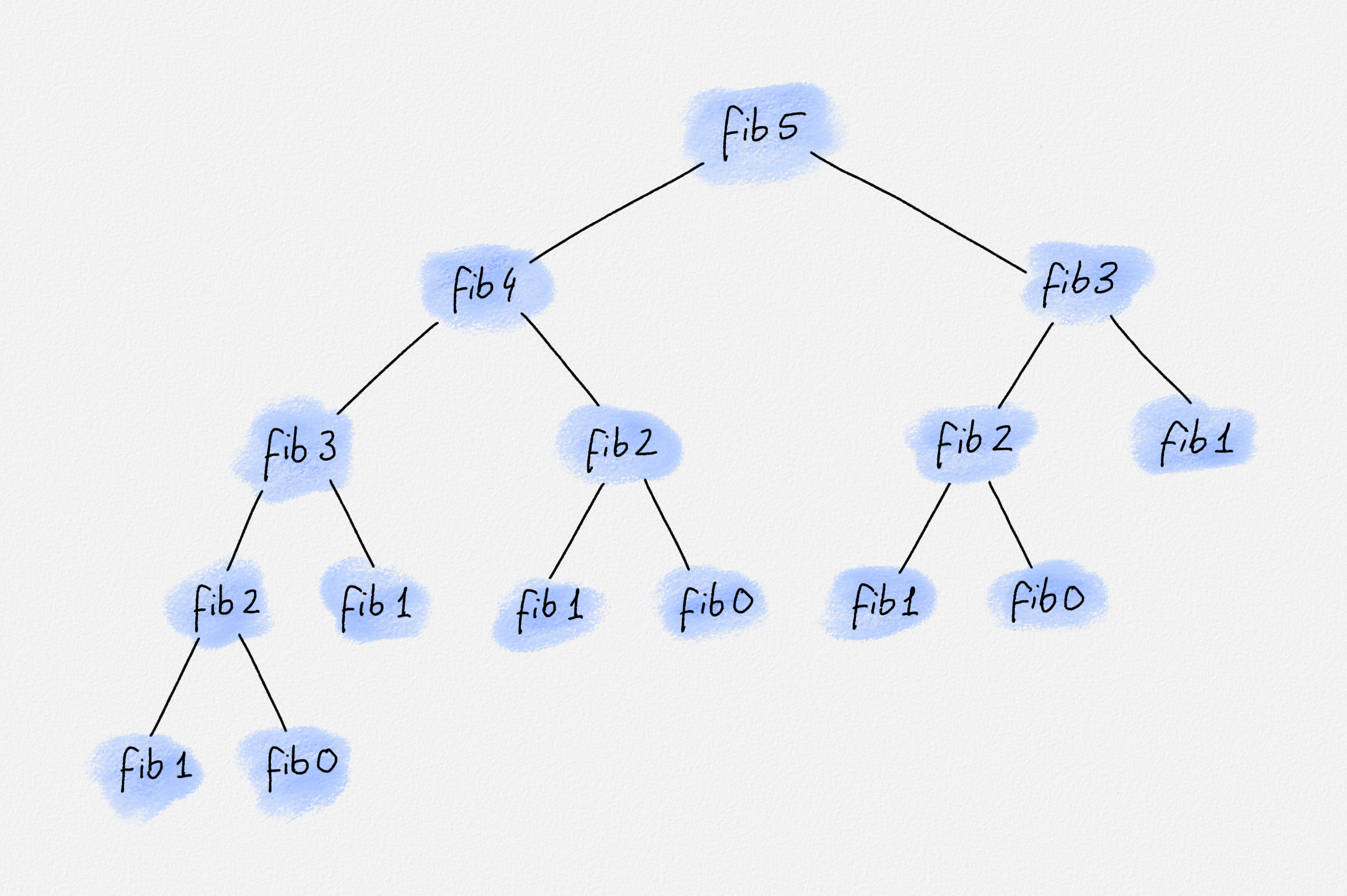
Recursion tree for fib 5
Thus, computing the \(n\)th Fibonacci number requires at least \(F_n\) addition operations. That's a whole lot of additions for \(F_{100}\), a number of additions that even today's computers won't finish in your lifetime. We'll discuss later how we can make computing Fibonacci numbers much faster, so we can compute even the 10,000th Fibonacci number in a flash:
>>> fib 10000
33644764876431783266621612005107543310302148460680063906564769974680081442166662
36815559551363373402558206533268083615937373479048386526826304089246305643188735
45443695598274916066020998841839338646527313000888302692356736131351175792974378
54413752130520504347701602264758318906527890855154366159582987279682987510631200
57542878345321551510387081829896979161312785626503319548714021428753269818796204
69360978799003509623022910263681314931952756302278376284415403605844025721143349
61180023091208287046088923962328835461505776583271252546093591128203925285393434
62090424524892940390170623388899108584106518317336043747073790855263176432573399
37128719375877468974799263058370657428301616374089691784263786242128352581128205
16370298089332099905707920064367426202389783111470054074998459250360633560933883
83192338678305613643535189213327973290813373264265263398976392272340788292817795
35805709936910491754708089318410561463223382174656373212482263830921032977016480
54726243842374862411453093812206564914032751086643394517512161526545361333111314
04243685480510676584349352383695965342807176877532834823434555736671973139274627
36291082106792807847180353291311767789246590899386354593278945237776744061922403
37638674004021330343297496902028328145933418826817683893072003634795623117103101
29195316979460763273758925353077255237594378843450406771555577905645044301664011
94625809722167297586150269684431469520346149322911059706762432685159928347098912
84706740862008587135016260312071903172086094081298321581077282076353186624611278
24553720853236530577595643007251774431505153960090516860322034916322264088524885
24331580515348496224348482993809050704834824493274537326245677558790891871908036
62058009594743150052402532709746995318770724376825907419939632265984147498193609
28522394503970716544315642132815768890805878318340491743455627052022356484649519
61124602683139709750693826487066132645076650746115126775227486215986425307112984
41182622661057163515069260029861704945425047491378115154139941550671256271197133
25276363193960690289565028826860836224108205056243070179497617112123306607331005
9947366875
For now, let's look at our second value we would like to compute, \(S_n\). Since
there already exists a sum function in the Haskell standard library, and s
is a bit short to be descriptive, let's call our function sumUpTo. Here's a
recursive definition:
sumUpTo :: Int -> Int
sumUpTo 0 = 0
sumUpTo n = sumUpTo (n - 1) + n
This doesn't feel quite as natural as a loop, but understanding this definition is a good exercise in thinking inductively, which is the key to writing code that repeats things via recursion.
What this function says is that the sum of the numbers from \(1\) up to \(0\) is
clearly \(0\), because there are no numbers between \(1\) and \(0\). If we want to
know the sum of the numbers from \(1\) up to some positive number \(n\), then that's
clearly the sum of the first \(n - 1\) numbers, sumUpTo (n-1), plus \(n\) itself.
Again, we can try this out, and this function works for reasonably large arguments:
>>> :l Sum.hs
[1 of 1] Compiling Main             ( Sum.hs, interpreted )
Ok, one module loaded.
>>> sumUpTo 10000000
50000005000000
It is not a very good implemention of sumUpTo, though, and we still have to
wait a little before the output of sumUpTo 10000000 appears. Every time we
make a recursive call, the state of this recursive call needs to be stored in
the form of a stack frame. Thus, computing sumUpTo 10000000 creates 10 million
stack frames to do something that we would have been able to do with very little
working space had we implemented it using a loop, as in Python:
def sum_up_to(n):
    sum = 0
    for i in range(0,n+1):
        sum += i
    return sum
The Python code ends up being much faster in this instance, exactly because it's a simple loop that doesn't make a massive number of recursive calls:
>>> from sum import *
>>> sum_up_to(10000000)
50000005000000
As I said, we don't have loops in Haskell. In the next section, we discuss how
to implement our sumUpTo function in a fashion that allows the compiler to
translate it back into a loop, so evaluating sumUpTo n once again uses a
constant amount of working space independent of the value of n. This tool is
called tail call optimization. At the end of this chapter, we will see
that we can also implement a tail-recursive version of our Fibonacci function,
one that computes large Fibonacci numbers blindingly fast.
Exercise
In Haskell, strings are just lists of characters. We can use pattern matching to distinguish between the empty string and a non-empty string:
someStringFunction ""     = ...
someStringFunction (x:xs) = ...
The pattern "" in the first equation matches the empty string. So this
equation is used to implement someStringFunction only when the argument is
the empty string. The pattern x:xs in the second equation matches any
non-empty string. Such a string can be described as follows: The string
starts with some character—this character must exist because the string is
not empty—and after this initial character comes the rest of the string,
which is itself a string of characters. The pattern x:xs takes the string
apart into these two components: x is the first character of the string.
xs is the remainder of the string and is, obviously, one character shorter
than the string x:xs. Note that when using : in a pattern, we need to
enclose the whole pattern in parentheses.
As in any pattern, we can use wildcards. For example, _:_ matches any
non-empty string, but we don't care at all about what that string looks
like. The pattern says that the string must have a head and a tail, which is
the same as saying that the string is non-empty. Of course, we can also use
a wildcard for ony one of the two components.
Implement two functions
isEmptyString :: String -> Bool
and
stringLength :: String -> Int
The former should statisfy isEmptyString "" = True and
isEmptyString s = False for any other string.
The latter should return the length of the string:
stringLength "Hello" = 5, for example.
Note: Since strings are just lists of characters and the standard
library already gives us functions null and length to test whether a
list is empty or what its length is, you could simply define
isEmptyString = null and stringLength = length. Indeed, Haskell
programmers simply use null and length for strings without defining
string-specific functions. As an exercise though, you should implement
isEmptyString and stringLength from scratch.
Solution
isEmptyString :: String -> Bool
isEmptyString "" = True
isEmptyString _  = False
This matches exactly the behaviour I said the function should require.
isEmptyString "" = True. isEmptyString _ = False is used for any string
that is non-empty because the pattern of the first equation does not match
for such strings.
stringLength :: String -> Int
stringLength (_:xs) = 1 + stringLength xs
stringLength _      = 0
Think about how we could define the length of a string:
- The empty string has length 0.
- The string
x:xscomposed of a characterxand tailxsclearly has one character more thanxs. Thus, its length is1 + stringLength xs.
Our first equation implements the second rule. We could have used the
pattern x:xs—that would work just fine—but we don't really care what
the first character looks like, only that it is present, so we use the
wildcard instead.
The second equation applies only if the pattern of the first equation
does not match. Thus, we know at this point that the string is empty
without inspecting the string. Thus, we get away with using the wildcard
as the pattern, and we return 0.
Exercise
Implement a function
countOccurrences :: Char -> String -> Int
countOccurrences x ys should count how often the character x occurs in
ys. For example, countOccurrences 's' "Mississippi" = 4 because there
are four 's's in "Mississippi".
Solution
countOccurrences :: Char -> String -> Int
countOccurrences x = go
  where
    go (y:ys) | x == y    = 1 + go ys
              | otherwise =     go ys
    go _                  = 0
This says that countOccurrence x is the same as the inner function
go. In other words, if we call countOccurrence x ys, this calls
go ys. If this makes no sense to you, read the section on
multi-argument functions
again.
Given a non-empty string y:ys, we have two cases. If x == y, then
the total number of occurrences of x in y:ys is clearly one more
than the number of occurrences of x in ys. go ys counts the latter
recursively, and then we add 1 to the result. If x /= y, the
otherwise branch, then all occurrences of x in y:ys must be in
ys. Thus, we call go ys recursively to count these occurrences.
If the string does not match the pattern y:ys of the first equation
for go, it must be the empty string. Thus, the second equation does
not even inspect the string and returns 0. Clearly, the empty string
contains no occurrence of x.
This definition is clearly correct, but it is not a very good definition. In the next section, you'll learn why and you will repeat this exercise to come up with a better definition.
Exercise
Newton's method can be used to compute good approximations of various functions efficiently. For example, here is how we approximate the square root of a number to within an error of 0.0001 in Python:
def square_root(x):
    root = x
    while True:
        quot = x / root
        if abs(quot - root) < 0.0001:
            return root
        root = (quot + root) / 2
So, we start by guessing that the root is x itself. When x = 1, this is
certainly true. Then we compute the quotient quot = x / root. If quot is
within 0.0001 of root, then root is close enough to being the true
square root of x, because quot * root = x and quot and root are
nearly identical. If abs(quot - root) > 0.0001, then the true root must
lie somewhere between quot and root, so we update root to the midpoint
between quot and root. You can try this out. It computes decent
approximations of the square root:
$ python3
>>> def square_root(x):
...     root = x
...     while True:
...         quot = x / root
...         if abs(quot - root) < 0.0001:
...             return root
...         root = (quot + root) / 2
...
>>> square_root(2)
1.4142156862745097
>>> square_root(4)
2.0000000929222947
>>> x = square_root(9)
>>> x * x
9.000000008381903
Implement this square_root function in Haskell.
Solution
squareRoot x = go x
  where
    go root | abs (root - quot) < 0.0001 = root
            | otherwise                  = go $ (root + quot) / 2
      where
        quot = x / root
We need something to simulate the while-loop of the Python function.
Since we don't have loops, we use recursion. We need to use an inner
function though, which we call go, because we need access to the
argument x of squareRoot in each "iteration". The argument of go
is our current estimate of the square root, root. Just as the Python
code starts with root = x, we call go with x as its argument.
go root computes quot = x / root in its where block. Remember, all
pattern guard branches of the definition of go can see the values
defined inside the where block. The first pattern guard tests whether
root and quot differ by at most 0.0001. If so, go returns root.
If not, we need to run for another iteration. We do this by calling go
recursively and returning whatever this recursive call returns. The
argument we pass to this recursive call is exactly the value to which
the Python code updates root: (root + quot) / 2. Note that
go (root + quot) / 2 would not work due to the precedence of function
calls and operator application. The expression go (root + quot) / 2 is
equivalent to (go (root + quot)) / 2. This would never terminate.
You can try that this function definition does the right thing:
>>> :{
  | squareRoot x = go x
  |   where
  |     go root | abs (root - quot) < 0.0001 = root
  |             | otherwise                  = go $ (root + quot) / 2
  |       where
  |         quot = x / root
  | :}
>>> squareRoot 2
1.4142156862745097
>>> squareRoot 4
2.0000000929222947
>>> x = squareRoot 9
>>> x * x
9.000000008381903
Note that this is not the only correct implementation. You could as well have used if-then-else, but Haskell programmers prefer pattern guards in most cases. Here's the implementation using if-then-else:
squareRoot x = go x
  where
    go root = let quot = x / root
              in  if abs (root - quot) < 0.0001 then
                      root
                  else
                      go $ (root + quot) / 2
What this implementation does have in common with the implementation above is that it uses recursion. It's the only way to repeat things in a purely functional language.
-
Even a Haskell fan boy like me often slips back into imperative lingo. Given that we don't specify steps to be executed in functional programs but we define the values of functions, the notion of "repeating steps" is in itself utter nonsense in functional languages. However, it seems impossible to compare the control flow constructs we have available in Haskell to those we are used to in imperative languages without describing the evaluation of Haskell functions in imperative terms. ↩
-
Code written in Haskell is nevertheless often slower than code written in C, C++ or Rust. Recursion is not to blame for this. The culprit is Haskell's lazy evaluation, which enables lots of elegant idioms but comes with a significant performance overhead. At the same time, Haskell code is by no means inefficient. To beat the performance of well-written Haskell code by a significant margin, you need to reach for C, C++ or Rust, with all the tedium involved in performance-oriented low-level programming. ↩