Where

The other mechanism for defining local variables is a where block:

veclen :: (Double, Double) -> Double
veclen (x, y) = sqrt (x2 + y2)
  where
    x2 = x * x
    y2 = y * y

Again, you can read this in English as "veclen (x, y) is sqrt (x2 + y2), where x2 is defined as x * x and y2 is defined as y * y". The scoping rules are exactly the same as for let blocks. The entire function definition, including its where block is one scope. Thus, the definition of the function value, sqrt (x2 + y2), and all definitions inside the where block can refer to all names defined inside the where block and to the function arguments. Of course, they can also refer to all names defined in surrounding scopes. And, once again, the order of the definitions in the where block is irrelevant:

GHCi

>>> :{
  | veclen (x, y) = sqrt sum
  |   where
  |     sum = x2 + y2
  |     x2  = x * x
  |     y2  = y * y
  | :}
>>> veclen (3,4)
5.0

For the most part, let blocks and where blocks are completely interchangeable in practice, and choosing between them is a matter of personal preference. Formally, they are slightly different beasts though:

let ... in ... is an expression. The scope of variables defined after let is this expression. In particular, let blocks can be nested within the same expression (even though this usually leads to less readable code):
GHCi
```
>>> :{
  | veclen (x, y) =
  |     let x2 = x * x
  |     in  let y2 = y * y
  |         in  let sum = x2 + y2
  |             in  sqrt sum
  | :}
>>> veclen (3,4)
5.0
```
Where is a clause attached to an equation: var = expr where .... Thus, you cannot nest where blocks unless the inner where block is attached to an equation in the outer where block. So this works:
GHCi
```
>>> :{
  | veclen (x,y) = sqrt sum
  |   where
  |     sum = x2 + y2
  |       where
  |         x2 = x * x
  |         y2 = y * y
  | :}
>>> veclen (3,4)
5.0
```

A consequence of where blocks being attached to equations, and let blocks being expressions is that they behave differently when using pattern guards. let blocks allow us to introduce different variable definitions for each equation after a pattern guard:

sillyFunction x
    | even x    = let y = 3 * x in y
    | otherwise = let y = 4 * x in y

Note that y = 3 * x in the first branch, and y = 4 * x in the second branch. Since the scope of the definitions introduced after let is the let ... in ... expression, these two definitions of let are not in conflict with each other.

Trying to do the same with where blocks doesn't work:

GHCi

>>> :{
  | sillyFunction x
  |     | even x    = y
  |         where y = 3 * x
  |     | otherwise = y
  |         where y = 4 * x
  | :}

<interactive>:82:5: error: parse error on input ‘|’

To understand why this doesn't work, it helps to remember that the definition of a function using multiple equations and pattern guards is just syntactic sugar for a single equation that uses a case expression. The above definition would be translated into

sillyFunction z = case z of
    x | even x    -> y
          where y = 3 * x
      | otherwise -> y
          where y = 4 * x

and suddenly we see why we have where blocks scattered through a single equation. On the other hand, the translation of the definition using let expressions is perfectly fine:

sillyFunction z = case z of
    x | even x    -> let y = 3 * x in y
      | otherwise -> let y = 4 * x in y

Exactly because let ... in ... is an expression.

So it seems that anything we can do with where blocks can also be achieved with let expressions, and let expressions are the more general tool that is generally preferable. This isn't quite true. Indeed, most Haskell programmers tend to use let expressions sparingly and tend to prefer where blocks. In most cases, this is a matter of aesthetics. In the case of pattern guards, it turns out that the need to provide different local definitions for the different branches (such as the two different definitions of y in our example above) arises infrequently. What does happen quite often is that we want to introduce variables that are shared across multiple branches with pattern guards. Given that a where block is attached to the whole equation, involving all the pattern guard branches, it exactly fits the bill. Here, for example, is an implementation of a function for pruning a binary tree:

data Tree a
    = Empty
    | Leaf a
    | Node (Tree a) (Tree a)

prune :: (a -> Bool) -> Tree a -> Tree a
prune _ Empty = Empty
prune pred (Leaf a)
    | pred a    = Leaf a
    | otherwise = Empty
prune pred (Node l r)
    | isEmpty l' = r'
    | isEmpty r' = l'
    | otherwise  = Node l' r'
  where
    l' = prune pred l
    r' = prune pred r

isEmpty :: Tree a -> Bool
isEmpty Empty = True
isEmpty _     = False

The use of an isEmpty function here is not the most idiomatic. It would be better to condense this down to a single case expression, but it'll do as a simple illustration. We also haven't discussed custom data types yet, but with a little help you'll appreciate the point this example makes:

The data type Tree a is a binary tree whose internal nodes do not store anything and whose leaves store values of some type a. Such a tree can have three different shapes. It can be Empty. It can be a Leaf storing a single value of type a. Or it can be an internal Node with two children. These two children themselves are Trees storing values of type a.

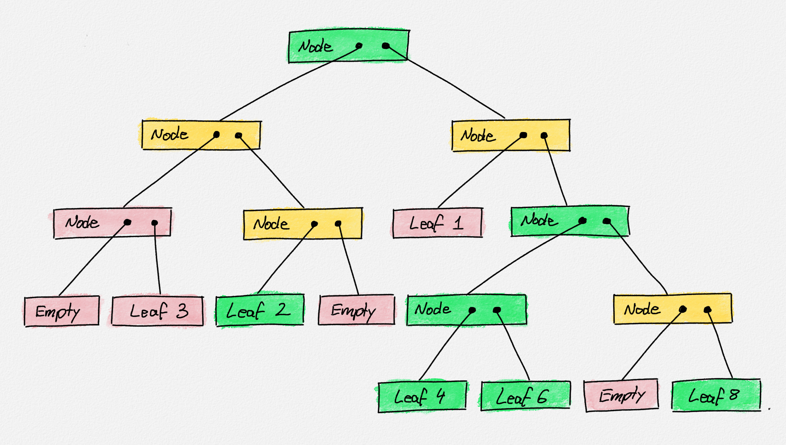
Example of a binary tree. The colouring of nodes will be explained in the next figure.

The prune function takes a Boolean predicate pred. Given such a predicate and a tree t, the idea is that we want to remove all leaves from t that do not match the predicate pred, and we want that the left and right subtrees of an internal Node are both non-empty; otherwise, at most one of the two subtrees stores any values, and the tree can be shrunk to only its left or right subtree.

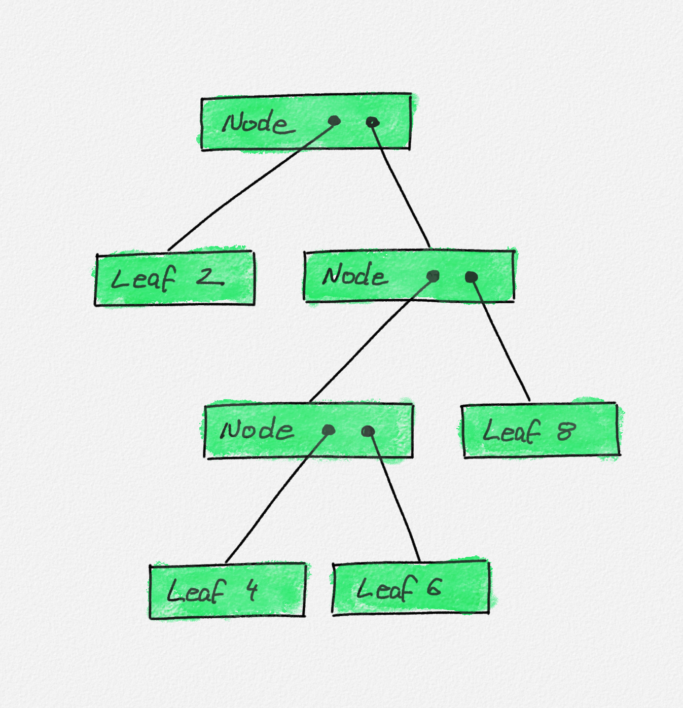
Result of pruning the tree in the previous figure — The result of pruning the tree in the previous figure using `prune even`, which keeps only leaves that store even numbers. The nodes in this tree are exactly the green nodes in the previous figures. Those are the leaves storing even numbers and the internal nodes that whose left and right subtrees both contain even numbers. The red nodes in the previous figure are removed: the invocation on those nodes produces an empty pruned tree. The yellow nodes are removed, but the invocation on those nodes does not produce an empty pruned tree. Each yellow node has one green and one red child. The invocation on a yellow node returns the green child.

The first equation for prune says that pruning an Empty tree produces an Empty tree no matter the predicate; so we use a wildcard for the predicate. The second equation prunes a tree consisting of a single leaf. In this case, the result is just this leaf if the value stored at the leaf matches the predicate pred; that's the | pred a = Leaf a branch. Otherwise, if the leaf does not match the predicate, then the result of pruning this tree is the Empty tree because its only leaf is removed. Finally—and this is the interesting part I want you to focus on here—if we want to prune a tree whose root is an internal Node with left child l and right child r, then we start by pruning l and r recursively. The two resulting trees are l' and r'. Now, if l' ends up being empty, then the whole tree should simply be whatever r' is (the | isEmpty l' = r' branch). If r' is empty, then the whole tree should be whatever l' is (the | isEmpty r' = l' branch). Otherwise, both l' and r' are non-empty, and we need to construct a new internal Node with left child l' and right child r' to obtain the final pruned tree. That's the | otherwise = Node l' r' branch.

The important point is that, to decide which of the three branches applies, we first need to prune l and r to produce l' and r'. The different branches of prune pred (Node l r) all use l' and r' in both the conditions we check to see whether these branches apply, and in defining the result of prune pred (Node l r) if this branch applies. A where clause makes this possible, because where introduces variables whose scope is the whole equation, including all of its pattern guard branches. If we wanted to use a let expression to do the same without recomputing l' or r' twice (which could be time-consuming if l and r are big subtrees), then the best we could do would be to translate the pattern guards into an if then else expression:

prune :: (a -> Bool) -> Tree a -> Tree a
prune _ Empty = Empty
prune pred (Leaf a)
    | pred a    = Leaf a
    | otherwise = Empty
prune pred (Node l r) =
    let l' = prune pred l
        r' = prune pred r
    in  if isEmpty l' then
            r'
        else if isEmpty r' then
            l'
        else Node l' r'

This is much harder to parse.

In the interest of completeness, here is how the seasoned Haskell programmer would implement prune:

prune :: (a -> Bool) -> Tree a -> Tree a
prune pred = pruneRec
  where
    pruneRec Empty = Empty
    pruneRec l@(Leaf a)
        | pred a    = l
        | otherwise = Empty
    pruneRec (Node l r) = case (pruneRec l, pruneRec r) of
        (Empty, r'   ) -> r'
        (l'   , Empty) -> l'
        (l'   , r'   ) -. Node l' r'

The pattern matching using a case expression in the third equation for pruneRec eliminates the need for the helper function isEmpty.

The use of an inner function pruneRec defined in the where block of prune ensures that we don't have to pass around the predicate pred to each recursive call. Instead, pruneRec has access to it because, as a local function defined inside prune, it has access to all arguments of prune (and to all values defined inside prune's where block).

Next, note that the equation of prune does not say prune pred t = pruneRec t. This would say that the result of applying prune to pred and t is the same as applying pruneRec to t. Instead, our definition says that prune pred is the same as the function pruneRec. Of course, these two function definitions are semantically equivalent, but once you're used to playing with partial function application in this way, you may find this way of defining functions more natural.

Finally, note the strange pattern in the second equation of pruneRec: l@(Leaf a). This is an "at-pattern" (because it uses the @ symbol). We'll return to it once we talk about data types. In a nutshell, it achieves two bindings at the same time: First, we bind the value stored at the leaf to the variable a. We need this to verify whether this value satisfies our predicate. Second, we bind the whole leaf to the variable l. This allows us to simply return the leaf l itself if it satisfies the predicate. Without the at-pattern, we would have had to reconstruct the leaf from the value it stores, by returning Leaf a. The difference is that the expression Leaf a would construct a new leaf storing the same value a that l stores. Instead, we simply return l itself. This makes the code more efficient.