Mini-Project: Fibonacci Numbers Revisited

We discussed two functions for computing Fibonacci numbers already. One was based directly on the recursive definition of these numbers but was inefficient. The other used tail recursion to obtain the result in linear time. Now we want to generate the sequence of all Fibonacci numbers

fibonaccis :: [Integer]

We use Integer, not Int, as the number type because Fibonacci numbers grow exponentially, so we really want a number type that can represent arbitrarily large numbers. Here is the whole definition of fibonaccis:

fibonaccis = 0 : 1 : zipWith (+) fibonaccis (tail fibonaccis)

Just as our intListTail function form earlier, tail fibonaccis returns the tail of fibonaccis, that is, the list fibonaccis with its first element removed. zipWith f xs ys is a list function we will meet again in the next chapter. It allows us to build a new list zs = zipWith f xs ys, where the first element in zs is obtained by applying the function f to the first element in xs and the first element in ys, the second element in zs is obtained by applying the function f to the second element in xs and the second element in ys, and so on:

zipWith :: (a -> b -> c) -> [a] -> [b] -> [c]
zipWith f = go
  where
    go (x:xs) (y:ys) = f x y : go xs ys
    go _      _      = []

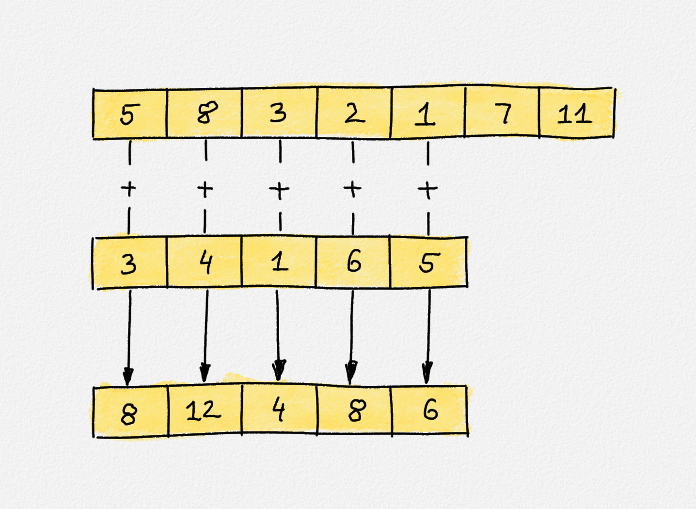
Illustration of zipWith — Illustration of the expression `zipWith (+) [5,8,3,2,1,7,11] [3,4,1,6,5]`. Note that the result has the same length as the shorter of the two argumment lists.

So our definition of fibonaccis says that the first list element, the 0th Fibonacci number $F_0$ is 0, the second list element is $F_1 = 1$, and the remainder of the sequence is obtained by zipping together fibonaccis with tail fibonaccis. Thus, the third element in the list, $F_2$, is obtained as the sum of the first element of fibonaccis, that is, $F_0$, and the first element of tail fibonaccis, that is the second element of fibonaccis, $F_1$. That's certainly correct. The fourth element, $F_3$, is obtained as the sum of the second element of fibonaccis, $F_1$, and the second element of tail fibonaccis, that is, the third element of fibonaccis, $F_2$. Again, this is correct. The following figure illustrates this and also shows that every list element depends only on the values of previous list elements. Thus, every list element can be computed in constant time if all the list elements before it have already been computed. The amortized cost per list element is constant.

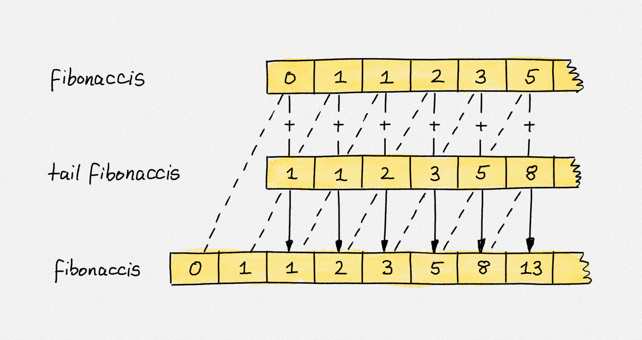
Illustration of definition of fibonaccis — Illustration of the computation of `fibonaccis`. The top copy of `fibonaccis` is the first argument to `zipWith (+)`. The middle row is `tail fibonaccis`, the second argument of `zipWith (+)`. The bottom copy of `fibonaccis` is the result of `0 : 1 : zipWith (+) fibonaccis (tail fibonaccis)`. The important part is that all these occurrences of `fibonaccis` refer to the exact same list. They are drawn as separate copies in this figure, but in memory, they are they same list, stored in the variable `fibonaccis`. Thus, the list entries linked by dashed lines in this figure are the exact same list node. This shows that the third element in `fibonaccis` is computed as the sum of the first and second elements in `fibonaccis`, the fourth element in `fibonaccis` is computed as the sum of the second and third elements in `fibonaccis`, and so on.

So a list can be defined using an expression that use the list itself as one or more of its arguments. You may sometimes hear the term "tying the knot" to refer to this technique, because in memory, we get an expression graph that has a cycle in it, a "knot". We have to be careful when we do this though. Haskell cannot magically compute values that depend on themselves:

GHCi

>>> x = 0 * x
>>> x
^CInterrupted.

We can define x as the number that is 0 multiplied by itself. This number is even well-defined because only 0 satisfies this condition. But our Haskell program still only follows pretty naïve instructions here: To compute x, we need to multiply 0 and x, so we need to know x. Thus, we go and compute x, which we do by multiplying 0 and x. To do this, we first need to know x. And so on. We have ourselves a nice infinite loop. The reason why we can build lists that are defined in terms of themselves is that lists are composed of individual list nodes. As long as each list node depends only on the values of other list nodes, and there is no cycle in the graph of these dependencies, we know how to evaluate each list node.¹ For our fibonaccis sequence, the first and second list nodes are given explicitly: 0 and 1. The third list node depends only on the first two list nodes. The fourth list node depends only on the second and third list node, and so on. There is no cycle in these dependencies. That's why this works.

The Haskell compiler would be perfectly happy to accept the following incorrect definition:

fibonaccisWrong = zipWith (+) fibonaccisWrong fibonaccisWrong

Only now we have a problem: To calculate the first element in fibonaccisWrong, we need to know the first element in fibonaccisWrong, as the first element is defined as the sum of two copies of the first element. We can define fibonaccisWrong, but if we ask even for only the first list element, the code gets stuck in an endless loop due to the dependence of each list element on itself. That's the same as with our attempt to evaluate x = 0 * x.

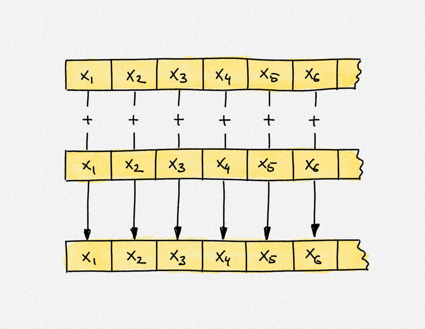
Illustration of fibonaccisWrong — Illustration of the definition of `fibonaccisWrong`. Each row shows a copy of `fibonaccisWrong`. The top two copies are the arguments of `zipWith (+)`. The bottom copy is the result of `zipWith (+) fibonaccisWrong fibonaccisWrong`. Once again, these lists are only *shown* as separate copies in this figure. They are in fact the exact same list. Thus, the first list element $x_1$ is produced by adding $x_1$ and $x_1$. The second list element $x_2$ is produced by adding $x_2$ and $x_2$. And so on. In particular, none of these list elements can be computed because evaluating the expression $x_1 = x_1 + x_1$, for example, results in an infinite recursion.

GHCi

>>> fibonacciWrong = zipWith (+) fibonacciWrong fibonacciWrong
>>> head fibonacciWrong
^CInterrupted.

To exit the endless loop, you need to press Ctrl+C.

If you instead try to view fibonaccis, GHCi happily prints lots of Fibonacci numbers on the screen. Of course, you need to get ready to press Ctrl+C once again to stop this process, because there are infinitely many numbers in the list to print. The point is that we don't get stuck in an endless loop when generating each individual list element.

To extract only the first 10 or 100 or 1,000 Fibonacci numbers, we can use a little helper function, take. take k xs returns the list containing only the first k elements of xs. If xs has fewer than k elements, then the result is all of xs. The implementation is straightforward:

take :: Int -> [a] -> [a]
take 0 _      = []
take _ []     = []
take k (x:xs) = x : take (k - 1) xs

With this function, we can inspect our Fibonacci sequence:

GHCi

>>> fibonaccis = 0 : 1 : zipWith (+) fibonaccis (tail fibonaccis)
>>> take 10 fibonaccis
[0,1,1,2,3,5,8,13,21,34]
>>> take 20 fibonaccis
[0,1,1,2,3,5,8,13,21,34,55,89,144,233,377,610,987,1597,2584,4181]

Exercise

Define the list of all powers of 2

powersOf2 :: [Integer]

and report the first 20 entries in this list.

Solution

There are a number of solutions. The most obvious one is

GHCi

>>> powersOf2 = map (2^) [0..]
>>> take 20 powersOf2
[1,2,4,8,16,32,64,128,256,512,1024,2048,4096,8192,16384,32768,65536,131072,262144,524288]

We apply the function (2^), that is, the function \x -> 2^x to each number in the list [0..]. Clearly, this produces the list of all powers of 2.

What I really had in mind was for you to mimic the implementation of fibonaccis:

GHCi

>>> powersOf2 = 1 : zipWith (+) powersOf2 powersOf2
>>> take 20 powersOf2
[1,2,4,8,16,32,64,128,256,512,1024,2048,4096,8192,16384,32768,65536,131072,262144,524288]

This is based on the following recursive definition of powers of 2:

\[ 2^n = \begin{cases} 1 & \text{if } n = 0\\ 2^{n-1} + 2^{n-1} & \text{otherwise} \end{cases} \]

Thus, the first element in the sequence is $2^0 = 1$. Each subsequent entry is produced by summing two copies of the element before it.

Finally, we could also start with the following recurrence:

\[ 2^n = \begin{cases} 1 & \text{if } n = 0\\ 2 \cdot 2^{n-1} & \text{otherwise} \end{cases} \]

This leads to the following definition:

GHCi

>>> powersOf2 = 1 : map (2*) powersOf2
>>> take 20 powersOf2
[1,2,4,8,16,32,64,128,256,512,1024,2048,4096,8192,16384,32768,65536,131072,262144,524288]

Again, we have $1$ as the first list element. Each subsequent element is obtained by applying the function (2*), that is, the function \x -> 2*x to the element before it.

It's actually a bit more complicated than this. We can define lists where the $i$th list entry depends on the $i$th list entry. This works as long as the list entries themselves are data structures and each of these data structures does not have any circular dependencies between its entries.

For example, here is a fairly convoluted way to generate the list of all binomial sequences: The first list in the list is the list $\bigl[\binom{0}{0}, \binom{1}{0}, \binom{2}{0}, \ldots\bigr] = [1,1,1,\ldots]$. The second list is $\bigl[\binom{1}{1}, \binom{2}{1}, \binom{3}{1}, \ldots\bigr] = [1,2,3,\ldots]$. The third list is $\bigl[\binom{2}{2}, \binom{3}{2}, \binom{4}{2}, \ldots\bigr] = [1,3,6,\ldots]$. And so on. In general, the $j$th entry in the $i$th list is $\binom{i+j}{i}$:
GHCi
```
>>> leftUpSum xs = let zs = zipWith (+) xs (0 : zs) in zs
>>> binoms = [1,1..] : map leftUpSum binoms
>>> mapM_ (putStrLn . show) $ take 10 $ map (take 10) binoms
[1,1,1,1,1,1,1,1,1,1]
[1,2,3,4,5,6,7,8,9,10]
[1,3,6,10,15,21,28,36,45,55]
[1,4,10,20,35,56,84,120,165,220]
[1,5,15,35,70,126,210,330,495,715]
[1,6,21,56,126,252,462,792,1287,2002]
[1,7,28,84,210,462,924,1716,3003,5005]
[1,8,36,120,330,792,1716,3432,6435,11440]
[1,9,45,165,495,1287,3003,6435,12870,24310]
[1,10,55,220,715,2002,5005,11440,24310,48620]    
```
The $i$th binomial sequence is computed from both the $(i-1)$st binomial sequence and the $i$th binomial sequence itself. The reason why this works is that the $j$th entry in the $i$th binomial sequence depends only on the $(j-1)$st entry in the $i$th binomial sequence. So, once again, at the level of individual entries, there are no circular dependencies.

A bit more formally, an expression e contains no cycles if it can be evaluated to WHNF without having to evaluate any part of e before this evaluation to WHNF, and each subexpression of e satisfies the same condition. ↩