M41: k-NN Intuition: Distance & Scaling
CSCI 1109 — Practical Data Science
Frank Rudzicz
Learning outcomes
By the end of this module, you should be able to:
- Explain the \(k\)-nearest neighbours (\(k\)-NN) idea using feature space and distance.
- Compute common distance measures (L2 / Euclidean; L1 / Manhattan) for simple feature vectors.
- Diagnose when feature scales or units make raw distances misleading.
- Apply basic feature scaling (standardization / min-max) and justify why it matters for \(k\)-NN.
- Predict and compare how changing distance metrics or scaling might change \(k\)-NN predictions in a small example.
Motivation: triaging patients in an emergency department
Imagine an emergency department that wants to flag patients at high risk of needing ICU care within the next 24 hours.
For each patient, we might have features like:
heart_rateoxygen_saturationrespiratory_ratetemperature_clactate_level
Label:
needs_icu(0 = no, 1 = yes)
k-NN idea:
“Find previous patients who look most similar in this feature space.
See what happened to them. Use that as our prediction.”
This is a high-impact decision: getting it wrong affects resource use and patient outcomes.
Conceptual scaffold
Feature space & neighbours
Feature vector
- For each patient \(i\), collect features into a vector: \[ \mathbf{x}^{(i)} = [x^{(i)}_1, x^{(i)}_2, \dots, x^{(i)}_d] \] where each coordinate is a feature (heart rate, oxygen, etc.)
Feature space
- A d-dimensional space where each axis is a feature.
- Each patient is a point in that space.
Nearest neighbours
- “Near” = small distance between feature vectors
- For a new patient \(\mathbf{x}^{(\text{new})}\), k-NN:
- Compute distance from \(\mathbf{x}^{(\text{new})}\) to every training point
- Pick the k closest points
- For classification: majority label among those neighbours
- For regression: average the neighbours’ target values
Nearest neighbours example
The plot shows:
- Blue circles = patients who did not need ICU
- Red circles = patients who did need ICU
- A gold star ★ = a new patient
- A ring around the \(k\) nearest neighbours of the star
Use the slider under the plot to:
- Change \(k\) and see which points are considered neighbours
Distances: informal intuition
Two common distance measures between vectors \(\mathbf{x}\) and \(\mathbf{z}\):
- L2 (Euclidean) — “as the crow flies”
- Usual straight-line distance
- Sensitive to large differences (squares)
- L1 (Manhattan) — “city-block distance”
- Sum of absolute differences
- Sometimes more robust to outliers
🔑 Key idea
distance is defined in feature space, not physical space.
We choose the metric that makes sense for our data and task.
Math lens
L2 / Euclidean distance
Definition:
\[ d_{L2}(\mathbf{x}, \mathbf{z}) = \sqrt{ \sum_{j=1}^d \left(x_j - z_j\right)^2 } \]
Example (2 features):
- Patient A: \(\mathbf{x} = [ \text{heart_rate}=90,\ \text{oxygen}=92]\)
- Patient B: \(\mathbf{z} = [ \text{heart_rate}=100,\ \text{oxygen}=89]\)
\[ \begin{aligned} d_{L2}(\mathbf{x}, \mathbf{z}) &= \sqrt{(90 - 100)^2 + (92 - 89)^2} \\ &= \sqrt{(-10)^2 + (3)^2} \\ &= \sqrt{100 + 9} = \sqrt{109} \approx 10.44 \end{aligned} \]
L1 / Manhattan distance
Definition:
\[ d_{L1}(\mathbf{x}, \mathbf{z}) = \sum_{j=1}^d \left|x_j - z_j\right| \]
Same patients:
- A: \(\mathbf{x} = [90, 92]\)
- B: \(\mathbf{z} = [100, 89]\)
\[ d_{L1}(\mathbf{x}, \mathbf{z}) = |90 - 100| + |92 - 89| = 10 + 3 = 13 \]
Both metrics say “these patients aren’t too far apart”—just slightly different ways of counting.
\(k\)-NN algorithm: step-by-step
Given:
- Training data: \((\mathbf{x}^{(i)}, y^{(i)})\) for \(i = 1, \dots, n\)
- New point: \(\mathbf{x}^{(\text{new})}\)
- Choice of:
- \(k\) (number of neighbours)
- Distance metric (e.g., L2)
Algorithm (classification)
- For each training example \(i\), compute distance
\(d_i = d(\mathbf{x}^{(\text{new})}, \mathbf{x}^{(i)})\). - Sort training points by distance \(d_i\).
- Take the \(k\) closest points.
- Let them vote: \(\hat{y} = \text{majority class among those $k$ labels}\).
- Return \(\hat{y}\) as the prediction.
Warning
No training step! k-NN is an instance-based / lazy learner.
❌ Anti-example: when distance lies to you (lab vs vitals)
Suppose we use features:
oxygen_saturation(70–100)lab_marker_crp(0–10,000, mg/L)
Three patients:
- Patient 1: \([92\ \text{oxygen}, 1{,}000 \ \text{CRP}]\)
- Patient 2: \([90\ \text{oxygen}, 2{,}000 \ \text{CRP}]\)
- Patient 3: \([80\ \text{oxygen}, 3{,}000 \ \text{CRP}]\)
Which is closer to Patient 1?
Clinically, a big drop in oxygen (say from 92 to 80) is serious.
In raw Euclidean distance:
- Oxygen differences are at most 12
- CRP differences are in thousands
The distance is dominated by
lab_marker_crp.
Even if oxygen levels are very different, CRP completely swamps them.
Warning
Raw distances on features with wildly different scales can be misleading, especially in medicine.
Why scaling matters
Take 2-feature vectors:
\[ \mathbf{x} = [x_{ \text{oxygen}}, x_{ \text{crp}}], \quad \mathbf{z} = [z_{ \text{oxygen}}, z_{ \text{crp}}] \]
Squared L2 distance:
\[ \begin{aligned} d_{L2}^2(\mathbf{x}, \mathbf{z}) &= (x_{ \text{oxygen}} - z_{ \text{oxygen}})^2 + (x_{ \text{crp}} - z_{ \text{crp}})^2 \end{aligned} \]
If CRP ranges from 0 to 10,000, then even a small relative difference in CRP (say 500) gives:
\[ (500)^2 = 250{,}000 \]
Compare that to oxygen: a difference of 5 percentage points gives
\[ (5)^2 = 25 \]
So CRP contributes 10,000× more to the distance.
Note
Without scaling, k-NN might act like “distance is in CRP only,” ignoring oxygen almost completely.
Review: scaling (from M16)
For the full math + code details on scaling, see the earlier module:
For this module, remember:
- Scaling can make distance-based models like \(k\)-NN behave sensibly.
- Use z-scores or min–max, fitted on the training data only, before running \(k\)-NN.
🔬 Stretch: effect of uniform scaling on neighbours
Suppose we scale all features by the same constant \(c > 0\):
\[ \mathbf{x}' = c \mathbf{x}, \quad \mathbf{z}' = c \mathbf{z} \]
Then:
\[ \begin{aligned} d_{L2}(\mathbf{x}', \mathbf{z}') &= \sqrt{\sum_j (c x_j - c z_j)^2} \\ &= \sqrt{\sum_j c^2 (x_j - z_j)^2} \\ &= c \sqrt{\sum_j (x_j - z_j)^2} \\ &= c \, d_{L2}(\mathbf{x}, \mathbf{z}) \end{aligned} \]
So all distances are multiplied by the same factor \(c\).
- The order of distances doesn’t change.
- So the set of nearest neighbours is the same.
Takeaway
- Uniform scaling (multiply all features by the same constant) does not affect neighbour ranking.
- The problem comes when we scale different features differently (which we usually do on purpose).
Worked example 1
Tiny 2D k-NN by hand (ICU risk)
We’ll build a toy dataset in 2D:
Code
| heart_rate | oxygen_sat | needs_icu | |
|---|---|---|---|
| 0 | 70 | 98 | 0 |
| 1 | 85 | 95 | 0 |
| 2 | 90 | 93 | 0 |
| 3 | 110 | 88 | 1 |
| 4 | 120 | 85 | 1 |
New patient: heart_rate=100, oxygen_sat=90. What does k-NN predict?
Compute distances
Code
| heart_rate | oxygen_sat | needs_icu | distance | |
|---|---|---|---|---|
| 3 | 110 | 88 | 1 | 10.198039 |
| 2 | 90 | 93 | 0 | 10.440307 |
| 1 | 85 | 95 | 0 | 15.811388 |
| 4 | 120 | 85 | 1 | 20.615528 |
| 0 | 70 | 98 | 0 | 31.048349 |
For k = 3, the neighbours are indices 3, 2, 1 with labels [1, 0, 0] → majority 0.
k-NN predicts: this patient does not need ICU-level care.
Warning
This is just a toy example; real clinical models would be carefully validated!
Simple plot
We can visualize the points and our new patient.
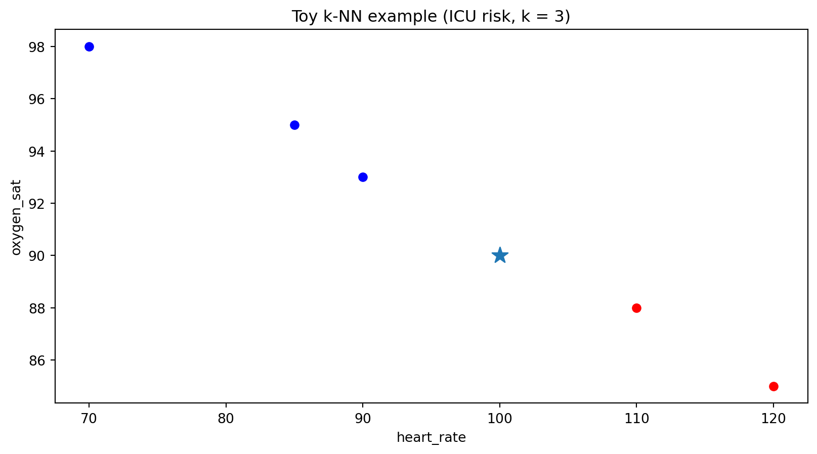
- Blue circles: patients who did not go to ICU
- Red circles: patients who did go to ICU
- Star ★: new patient at (100, 90)
Effect of changing \(k\) (conceptual)
Using the same toy dataset:
- If \(k = 1\): only the single closest neighbour (index 3 → label 1)
- If \(k = 3\): neighbours → [1, 0, 0] → majority 0
- If \(k = 5\): all points → [1, 0, 0, 1, 0] → majority 0
In real systems:
- Small \(k\) → more sensitive to noise (high variance, low bias)
- Large \(k\) → smoother, may miss small but real patterns (lower variance, higher bias)
- If you can sweep \(k\) using the validation set and observe that the decision becomes stable, this may be a good sign.
We’ll explore hyperparameters more in other modules.
Worked example 2
Scaling changes neighbours (infection risk)
Unscaled distances (numerical)
Code
| temp_c | crp | needs_antibiotics | distance | |
|---|---|---|---|---|
| 1 | 38.5 | 200 | 1 | 100.001250 |
| 2 | 39.2 | 10 | 0 | 290.002483 |
| 0 | 37.0 | 5 | 0 | 295.001695 |
| 3 | 36.8 | 1500 | 1 | 1200.000600 |
Rough distance intuition
- Temperature ranges over a few degrees, CRP over a thousand.
- For example, compare to patient 0 (37.0, 5):
- temp diff ≈ 1.0 → contributes 1
- CRP diff ≈ 295 → contributes 87,025 before sqrt
So whichever patient has CRP closest to 300 will be nearest, regardless of temperature.
Scaling then \(k\)-NN in scikit-learn
Use standardization for both features and use 🔗 KNeighborsClassifier:
Code
from sklearn.preprocessing import StandardScaler
from sklearn.neighbors import KNeighborsClassifier

X_train = patients2[["temp_c", "crp"]]
y_train = patients2["needs_antibiotics"]

scaler = StandardScaler()
X_train_scaled = scaler.fit_transform(X_train)

knn = KNeighborsClassifier(n_neighbors=3, metric="euclidean")
knn.fit(X_train_scaled, y_train)

# scale the new patient using *training* stats
new_scaled = scaler.transform([[38.0, 300]])
pred = knn.predict(new_scaled)
pred_proba = knn.predict_proba(new_scaled)

pred, pred_proba
(array([0]), array([[0.66666667, 0.33333333]]))pred_probagives probabilities for the two classes.
🔑 Key idea
After scaling, both temperature and CRP matter to the notion of “closeness”.
Evaluation & quality checks
For k-NN (like any model):
- We care about performance on unseen data, so we:
- Use train/validation/test splits (M38 reminder)
- Tune k and scaling only using train + validation, not test (avoid leakage from M40)
Common metrics (classification):
- Accuracy = fraction of correctly classified cases
- In high-impact settings (medicine, infrastructure):
- We also care about precision, recall, and the costs of false positives/negatives
- Missing a true ICU case is worse than one extra false alarm
Questions to ask:
- Is our model better than a simple baseline (e.g., always predict “no ICU”)?
- Does scaling improve validation accuracy?
- Are there particular subgroups (e.g., older patients) where performance is worse?
Summary
Ethics & risks: distance & fairness in high-stakes decisions
Even simple models like k-NN can cause harm if used carelessly:
- Sensitive features
- If we include features like
race,disability_status, orpostal_code, “closeness” may encode social biases. - Model might treat people as “similar” in ways that reflect historic discrimination.
- If we include features like
- Unequal error costs
- In medicine, false negatives (missing high-risk patients) can be deadly.
- In social services, false positives might lead to over-policing certain communities.
- Mitigations at this level
- Be explicit about which features you include and why.
- Try simple group-wise fairness checks: compare error rates for different subgroups.
- Think about the decision context: who is helped or harmed by false positives / false negatives?
Curiosity: \(k\)-NN in the wild
Although \(k\)-NN is often a “toy” model in courses, its ideas show up in many systems:
- Medical decision support (Wang et al. 2022)
- Suggesting treatments by finding patients with similar clinical profiles in historical data.
- Infrastructure monitoring (Mehrabadi et al. 2025)
- Flagging bridges or transformers whose sensor patterns look like past failure cases.
- Epidemiology (Hong et al. 2021)
- Grouping regions with similar infection patterns to understand spread and interventions.
\(k\)-NN is a good mental model for “similarity-based retrieval”, even when the actual model is more complex.
Curiosity: from k-NN to explainability
Some “explainable AI” methods borrow ideas from k-NN:
- To explain a complex model’s prediction for one instance:
- Find nearby examples in feature space
- Show how the model acted on those cases (Chen et al. 2019)
- Fit a simple local model near the point (e.g., a small linear model around a neighbourhood) (Ribeiro, Singh, and Guestrin 2016)
Note
k-NN is not like those other models; however, it can be a way of thinking about local behaviour of complex systems.
Quick-check questions
Conceptual (MCQ)
Suppose we run k-NN on two features:oxygen_saturation(70–100) andcrp(0–200,000). We don’t scale either feature. Which is most likely?A. Oxygen and CRP contribute equally to distance.
B. CRP will dominate distance calculations.
C. Oxygen will dominate distance calculations.
D. It depends only on k, not on feature scales.Computation (short)
Compute the L2 distance between \(\mathbf{x} = [37.0, 5]\) and \(\mathbf{z} = [39.0, 15]\).Scaling (MCQ)
We standardize each feature using training data (subtract mean, divide by std). How does this affect k-NN?A. It leaves distances unchanged for every pair of points.
B. It can change which points are nearest neighbours.
C. It always makes the model worse.
D. It only matters for regression, not classification.Conceptual (short)
Explain in one sentence why we must fit the scaler on the training data only, then apply it to validation/test data.
Summary
- \(k\)-NN predicts by looking at the nearest neighbours in feature space.
- Distance metrics (L1, L2, etc.) define what “near” means.
- Feature scaling is crucial so that no single feature’s units dominate.
- \(k\)-NN is simple but powerful as:
- A first supervised model
- A mental model for similarity and local behaviour
References
Chen, Chaofan, Oscar Li, Chaofan Tao, Alina Jade Barnett, Jonathan Su, and Cynthia Rudin. 2019. “This Looks Like That: Deep Learning for Interpretable Image Recognition.” In Advances in Neural Information Processing Systems. Vol. 32.
Hong, Kwan, Sujin Yum, Jeehyun Kim, Daesung Yoo, and Byung Chul Chun. 2021. “Epidemiology and Regional Predictors of COVID-19 Clusters: A Bayesian Spatial Analysis Through a Nationwide Contact Tracing Data.” Frontiers in Medicine 8: 753428. https://doi.org/10.3389/fmed.2021.753428.
Mehrabadi, Fatemeh A., Andy Nguyen, Panam Zarfam, Maryam Bitaraf, and Armin Aziminejad. 2025. “Data-Efficient Anomaly Detection in Bridge Structures Using Weighted k-Nearest Neighbor Classifier.” Smart Materials and Structures 34 (11): 115044. https://doi.org/10.1088/1361-665X/ae1bed.
Ribeiro, Marco Tulio, Sameer Singh, and Carlos Guestrin. 2016. ““Why Should i Trust You?”: Explaining the Predictions of Any Classifier.” In Proceedings of the 22nd ACM SIGKDD International Conference on Knowledge Discovery and Data Mining, 1135–44. ACM. https://doi.org/10.1145/2939672.2939778.
Wang, Ni, Muyu Wang, Yang Zhou, Honglei Liu, Lan Wei, Xiaolu Fei, and Hui Chen. 2022. “Sequential Data-Based Patient Similarity Framework for Patient Outcome Prediction: Algorithm Development.” Journal of Medical Internet Research 24 (1): e30720. https://doi.org/10.2196/30720.