Operationalized Machine Learning in Healthcare

Lec 3: Honest models and meaningful evaluation

Frank Rudzicz

DGIN 5401 · Dalhousie University

1 · Define the study and earn a baseline

A professional workflow

Step Question Evidence you should provide
Define What exactly is the prediction study? data card, time zero, outcome window, split diagram
Constrain What complexity can the information support? event-count rationale, baseline, learning curve
Evaluate Do risks mean what they say in the target setting? discrimination, calibration, uncertainty, workload
Extend What changes when time or text changes the task? revised estimand, output contract, evaluation plan
Act What action and claim can the evidence justify? threshold scenarios, utility, limitations, audit trail

A professional deliverable

The model is one component. It should be embedded in a defensible chain from care context all the way to possible action.

🤔 Retrieve

Sketch, from memory:

  • population and unit of analysis;
  • index time and feature-availability cut-off;
  • outcome window;
  • train/validation/test split unit;
  • one data-generation mechanism that could create bias.

Start with a data card

For the AIRO-Sim example, define:

  • row: one eligible cardiac surgery;
  • identifier: surgery ID plus patient ID;
  • index time: end of surgery;
  • features: values available and finalized by that time;
  • target: qualifying SSI within 30 days;
  • site/time variables: retained for evaluation and monitoring;
  • text: notes available by the cut-off, with provenance;
  • exclusions: documented before any modelling.

Baseline 0: predict the base rate

For binary outcome prevalence \(\bar y\), the constant probability model predicts:

\[ \hat p_i=\bar y_{train}. \]

This baseline can have high accuracy when SSI is rare, yet provide no real discrimination.

This provides a worst possible case for log loss, Brier score, calibration, and expected counts.

Baseline 1: regularized logistic regression

\[ z_i=\mathbf{x}_i^\top\mathbf{w}+b, \qquad \hat p_i=\sigma(z_i) \]

Here, \(\sigma(\cdot)\) is the sigmoid function and describes a function on \([0,1]\).

Why begin here?

  • strong baseline for tabular clinical data;
  • fast, reproducible, and easy to inspect;
  • supports regularization and calibrated risk estimation;
  • exposes data problems before architectural complexity;
  • provides a useful comparator (sometimes, for the status quo) even when a more complex model wins.

Linear regression refresher

For continuous outcome \(y\), the prediction is:

\[ \hat y_i=\beta_0+\sum_j\beta_jx_{ij} \]

Mean squared error:

\[ \text{MSE}=\frac{1}{n}\sum_i(y_i-\hat y_i)^2. \]

The coefficients describe changes in the fitted conditional mean under the model’s assumptions. These are not necessarily causal effects.

Logistic loss

For a binary target \(y_i\in\{0,1\}\):

\[ \ell_i=-\left[y_i\log \hat p_i+(1-y_i)\log(1-\hat p_i)\right]. \]

This loss strongly penalizes confident wrong predictions and encourages probability estimates rather than only hard labels.

Risk

Optimizing log loss does not choose a clinically appropriate threshold or guarantee subgroup calibration. By itself, it’s a very generic approach.

Underfitting and overfitting

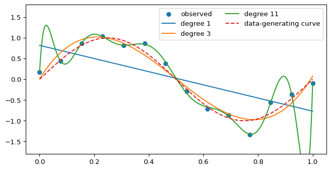
For one predictor, polynomial regression generalizes the linear model by adding powers of (x):

\[ \hat y^{(d)}(x) = \beta_0+\beta_1x+\beta_2x^2+\cdots+\beta_dx^d = \sum_{j=0}^{d}\beta_jx^j. \]

The degree \(d\) controls flexibility. The model is nonlinear in \(x\), but still linear in the fitted coefficients \(\beta_j\).

Underfitting and overfitting

Code
rng = np.random.default_rng(5401)
x = np.linspace(0, 1, 14)
y_true = np.sin(2*np.pi*x)
y = y_true + rng.normal(0, .18, size=len(x))
xx = np.linspace(0,1,400)
fig, ax = plt.subplots(figsize=(8,4))
ax.scatter(x,y,label="observed")
for deg in [1,3,11]:
    coef = np.polyfit(x,y,deg)
    ax.plot(xx,np.polyval(coef,xx),label=f"degree {deg}")
ax.plot(xx,np.sin(2*np.pi*xx),linestyle="--",label="data-generating curve")
ax.set_ylim(-1.8,1.8)
ax.legend(ncol=2)
plt.show()
  • too simple: misses stable structure;
  • too flexible: follows noise and idiosyncrasies;
  • the right complexity depends on data amount, noise, shift, and objective.

Regularization expresses a preference

Solution: make the weights themselves smaller, to reduce big fluctuations

Ridge / \(L_2\) penalty:

\[ \mathcal{J}=\mathcal{L}+\lambda\frac{1}{2}\sum_j\beta_j^2. \]

Lasso / \(L_1\) penalty:

\[ \mathcal{J}=\mathcal{L}+\lambda\sum_j|\beta_j|. \]

Regularization can reduce variance and stabilize estimates, but it does not rescue poor labels, leakage, or non-representative data.

Validation to tune; test once

  • Training set: fit parameters and preprocessing.
  • Validation set: choose hyperparameters (like \(\lambda\)), features, thresholds, and calibration strategy.
  • Test set: estimate performance of the frozen pipeline.
  • External set: evaluate transportability in a new time, site, or population.

Risk

Repeatedly checking the test set turns it into another validation set and invalidates your results.

Why random row splits can misinform

Each simulated patient contributes four similar records.

A random row split allows the model to encounter some visits from a patient during training and other visits during testing, whereas the patient-held-out split test (and therefore tests generalizability) with genuinely unseen people.

Code
rng = np.random.default_rng(5401)
n_patients = 220
visits = 4
patient_signal = rng.normal(size=n_patients)
y_patient = (patient_signal + rng.normal(scale=.7,size=n_patients) > 0).astype(int)
X = np.repeat(patient_signal, visits)[:,None] + rng.normal(scale=.08,size=(n_patients*visits,1))
y = np.repeat(y_patient, visits)
patient_id = np.repeat(np.arange(n_patients), visits)

# A nearest-neighbour-style memorization score for illustration
perm = rng.permutation(len(y))
cut = int(.7*len(y))
tr, te = perm[:cut], perm[cut:]
pred_random = np.array([y[tr[np.argmin(abs(X[tr,0]-X[i,0]))]] for i in te])
acc_random = (pred_random==y[te]).mean()

train_patients = np.arange(0,150)
test_patients = np.arange(150,n_patients)
tr2 = np.where(np.isin(patient_id,train_patients))[0]
te2 = np.where(np.isin(patient_id,test_patients))[0]
pred_group = np.array([y[tr2[np.argmin(abs(X[tr2,0]-X[i,0]))]] for i in te2])
acc_group = (pred_group==y[te2]).mean()
print({"random-row accuracy": acc_random, "patient-held-out accuracy": acc_group})
{'random-row accuracy': np.float64(0.7613636363636364), 'patient-held-out accuracy': np.float64(0.7071428571428572)}

Repeated records from one patient can let a model recognize the patient rather than learn a portable clinical pattern.

2 · Let the information budget constrain the model

Rare outcomes: count events, not rows

Suppose a registry contains 3,000 surgeries and the 30-day SSI rate is 2%.

60 events

Those 60 events specifically may carry much of the information about how predictors relate to SSI than the other 2940 rows.

Now ask:

  • how many candidate parameters or nonlinear patterns are being estimated?
  • how many events are available in each time split and subgroup?
  • how much optimism (overestimation) should we expect?
  • how precise can calibration and threshold estimates possibly be?

How much data do we need? Heuristics like “10 events per variable” are not universal design solutions. Use formal sample-size planning and shrinkage principles appropriate to the intended model and estimand. (Efthimiou et al. 2024; Riley, Debray, et al. 2024)

Model complexity must be earned by information

Signals of excess complexity

  • large gap between apparent and validated performance;
  • unstable selected features or explanations;
  • extreme risk estimates;
  • calibration slope far from 1 (Stevens and Poppe 2020);
  • large uncertainty across resamples;
  • implausible subgroup behaviour.

Defences

  • prespecification and dimensionality reduction;
  • penalization or shrinkage;
  • bootstrap or nested resampling;
  • simple baselines and learning curves;
  • temporal validation;
  • honest uncertainty and reduced claims.

A (too-)flexible model can match the particular rare events in the training data very closely, while learning patterns that are too sample-specific to predict new patients reliably.

Model families, not a model zoo

Family Strengths Questions to ask
Regularized regression / GAM stable baseline, additive effects, inspectable are interactions or nonlinearity essential?
Trees / boosting nonlinearities, interactions, tabular performance calibration, missingness behaviour, shift?
Neural networks representation learning, multimodal data data scale, optimization, maintenance, explanation?
Survival / longitudinal models time-to-event and repeated data censoring, landmarks, dynamic validation?
Foundation / generative models flexible text and multimodal interfaces factuality, privacy, versioning, prompt dependence?

Generalized additive models

\[ g(E[Y\mid X])=\beta_0+f_1(x_1)+\cdots+f_p(x_p) \]

GAMs allow nonlinear univariate effects while preserving an additive structure that can be plotted.

They can be an excellent middle ground between linear models and opaque high-capacity models, especially when decision-makers need stable, reviewable risk functions. (Caruana et al. 2015)

Trees and gradient boosting

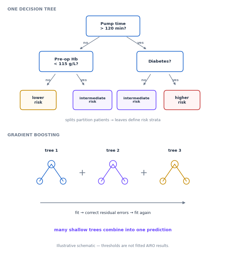
Decision trees partition features into rules. Trees can also be ‘ensembled’.

👍️ Advantages:

  • model interactions and nonlinearities;
  • handle mixed tabular features;
  • often strong performance on moderate-sized registries.

👎️ Risks:

  • overfitting and unstable feature importance;
  • poor probability calibration;
  • reliance on missingness or site artifacts;
  • explanations that are local summaries rather than mechanisms.

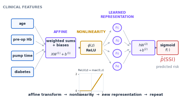
A neural network is repeated affine transformation plus nonlinearity

\[ \mathbf{h}^{(1)} = \phi\!\left(XW^{(1)}+\mathbf{b}^{(1)}\right), \qquad \hat y = f\!\left(\mathbf{h}^{(1)}W^{(2)}+\mathbf{b}^{(2)}\right). \]

What each layer does

\(XW+\mathbf b\) forms weighted combinations of the current features. The activation \(\phi(\cdot)\) introduces nonlinearity. Without it, stacked affine layers collapse mathematically to a single affine transformation.

Hidden layers \(\mathbf h^{(l)}\) learn representations useful for the training objective.

Additional layers can support increasingly complex learned representations.

Depth is not clinical knowledge

A deeper network may learn a useful representation, a shortcut, or noise. Clinical meaning comes from the data, labels, constraints, validation, and intended use—not from depth itself.

Why deep learning can help

Deep models are useful when patterns are distributed across high-dimensional inputs such as:

  • images;
  • waveforms and audio;
  • long sequences of measurements;
  • free text;
  • multimodal combinations.

Classic successes in dermatology and retinal imaging demonstrated the capacity of convolutional networks, while later work emphasized external evaluation and workflow integration. (Esteva et al. 2017; Gulshan et al. 2016; Beede et al. 2020)

Why deep learning can fail

Methodological reviews repeatedly identify leakage, weak external validation, and inappropriate comparisons. (Varoquaux and Cheplygina 2022; Kapoor et al. 2024)

Balancing classes, unbalance probabilities

Oversampling, undersampling, SMOTE (Chawla et al. 2002), or class weighting may change the training distribution.

Possible benefit

The learner pays more attention to rare examples or a chosen classification loss.

Common cost

Predicted probabilities no longer correspond to the target population without correction and recalibration.

In simulations and clinical examples, common imbalance corrections produced strong overprediction without improving discrimination; similar sensitivity/specificity trade-offs could be achieved by changing the threshold instead. (Goorbergh et al. 2022)

Separate three choices

How to train, how to estimate risk, and where to place a decision threshold are not the same problem.

Any resampling happens in training

flowchart LR
  A[Original development data] --> B[Outer train fold]
  A --> T[Untouched validation / test fold]
  B --> R[Resample or reweight only here]
  R --> M[Fit preprocessing and model]
  M --> T
  T --> E[Evaluate at natural prevalence]

Never oversample before splitting. Synthetic minority examples derived from validation or test observations leak information across the boundary.

3 · Evaluate risk estimates honestly

Confusion matrices

Predicted high risk Predicted low risk
SSI occurs True positive False negative
SSI does not occur False positive True negative
  • false positive (Type I error): extra calls, visits, anxiety, or treatment;
  • false negative (Type II error): missed enhanced surveillance;
  • true positive: benefit only if the action is effective and delivered;
  • true negative: may still require standard care.

Core binary metrics

\[ \text{Sensitivity}=\frac{TP}{TP+FN},\qquad \text{Specificity}=\frac{TN}{TN+FP} \]

\[ \text{Precision}=\frac{TP}{TP+FP},\qquad \text{NPV}=\frac{TN}{TN+FN} \]

Sensitivity and specificity condition on outcome status. Precision and NPV depend strongly on prevalence and the evaluation setting.

Accuracy can reward doing nothing

If SSI prevalence is 3%, predicting “no SSI” for every surgery yields 97% accuracy.

Report at least:

  • event prevalence and counts;
  • sensitivity and specificity at chosen thresholds;
  • precision and negative predictive value;
  • AUROC and AUPRC where appropriate;
  • calibration and proper scoring rules;
  • uncertainty and subgroup performance;
  • workload and clinical utility.

ROC and P/R answer different questions

  • ROC curve: sensitivity versus false-positive rate across thresholds.
  • PR curve: precision versus recall across thresholds.
  • AUROC: ranking probability for a random positive/negative pair.
  • AUPRC: performance focused on positive predictions; baseline depends on prevalence.

Risk

Neither curve selects the threshold or tells you whether the resulting action is worthwhile.

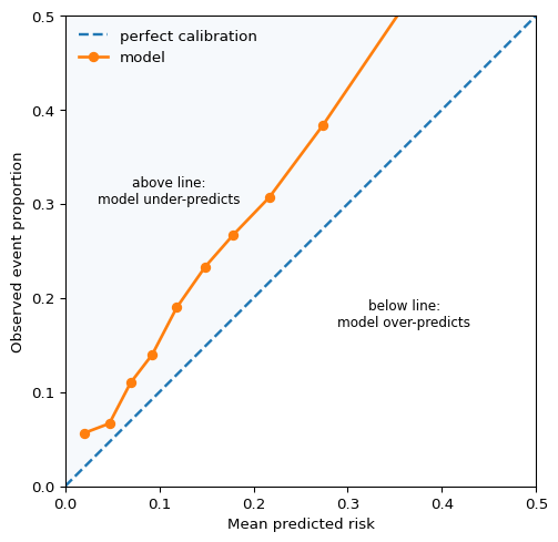
Calibration: are predicted risks realistic?

metric mistake

A model can rank patients well but still give poor probability estimates \(\hat p\). Calibration asks, e.g.:

Among patients assigned a predicted risk of about 10%, do about 10% actually experience the outcome?

For perfect calibration,

\[ P(Y=1 \mid \hat p=p) \approx p. \]

Calibration is not discrimination

A model can distinguish higher-risk from lower-risk patients well and still assign the wrong absolute probabilities. If a predicted 20% risk actually corresponds to 35% observed risk, a threshold or clinical decision based on that number may be badly misleading.

Calibration should also be examined in the population, place, and time in which the model is intended to be used. (Van Calster et al. 2016; Collins, Dhiman, et al. 2024)

Calibration: are predicted risks realistic?

The plot groups patients with similar predicted risks. For each group, it compares the mean predicted risk with the observed event proportion.

How to read the graph

  • The dashed 45° line represents perfect calibration: a predicted risk of 20% corresponds to an observed event rate of about 20%.
  • In this simulation, the calibration curve lies mostly above the diagonal because the outcome process was deliberately constructed so that actual risk is higher than predicted risk.

Two useful numerical summaries are:

  • Calibration intercept: captures systematic under- or over-prediction overall. Ideal value: (0).
  • Calibration slope: captures whether predicted risks are too extreme or not extreme enough. Ideal value: (1). A slope below (1) commonly indicates predictions that are too extreme, as can occur with overfitting.

Useful scoring rules

Brier score:

\[ \text{Brier}=\frac{1}{n}\sum_i(\hat p_i-y_i)^2. \]

Log loss:

\[ -\frac{1}{n}\sum_i[y_i\log\hat p_i+(1-y_i)\log(1-\hat p_i)]. \]

Both reward accurate probability estimates and penalize overconfidence. Compare them with a baseline (e.g., prevalence-only) and report uncertainty.

Thresholds convert risk into work

metric mistake
Code
rng = np.random.default_rng(7)
n = 1200
p = rng.beta(1.2, 14, size=n)
y = rng.binomial(1, np.clip(.01 + 1.6*p,0,.8))
rows=[]
for t in [.03,.05,.08,.12,.20]:
    pred=p>=t
    tp=((pred)&(y==1)).sum(); fp=((pred)&(y==0)).sum(); fn=((~pred)&(y==1)).sum()
    rows.append({"threshold":t,"flagged":int(pred.sum()),"TP":int(tp),"FP":int(fp),"FN":int(fn)})
pd.DataFrame(rows)
threshold flagged TP FP FN
0 0.03 879 152 727 13
1 0.05 686 137 549 28
2 0.08 455 111 344 54
3 0.12 246 75 171 90
4 0.20 74 32 42 133

Pause and discuss

At these thresholds, who is asked to do what—and how often?

A threshold is an error-cost decision

A threshold is an error-cost decision

The observed outcome does not change when the threshold moves; the decision classification does.

Lowering the threshold creates more alerts: some false negatives become true positives, while some true negatives become false positives. Raising it reverses those changes.

Move the slider and watch what changes:

  • lower threshold: more alerts; FN may become TP, while TN may become FP;
  • higher threshold: fewer alerts; TP may become FN, while FP may become TN.

The decision depends on the downstream consequences:

\[ \operatorname{cost}(t) = c_{\mathrm{FN}}\operatorname{FN}(t) + c_{\mathrm{FP}}\operatorname{FP}(t). \]

Threshold selection should involve the people who bear the workload and harm.

Decision curves and net benefit

metric mistake

Decision-curve analysis compares the value of model-guided action with “act on all” and “act on none,” weighting false positives according to a threshold probability. (Vickers, Van Calster, and Steyerberg 2016)

\[ \text{Net benefit}=\frac{TP}{N}-\frac{FP}{N}\frac{p_t}{1-p_t}. \]

Risk

Net benefit is only meaningful when the threshold encodes a defensible trade-off and the proposed action matches the analysis.

Claim uncertainty, certainly!

Report confidence intervals or resampling distributions for:

  • discrimination metrics;
  • calibration intercept and slope;
  • sensitivity, specificity, and precision at chosen thresholds;
  • subgroup differences;
  • net benefit;
  • individual risk estimates when they are used directly;
  • (basically whenever you can).

Small event counts can make apparently precise model outputs highly uncertain. (Riley et al. 2025; Riley, Debray, et al. 2024)

Subgroup evaluation

Pre-specify clinically and socially relevant groups, then report:

  • sample and event counts;
  • missingness and follow-up;
  • discrimination and calibration;
  • threshold-specific error rates;
  • uncertainty;
  • whether the same action and threshold are appropriate;
  • intersectional groups where feasible.

Chest-radiograph studies illustrate that underdiagnosis can be systematically concentrated in underserved populations. (Seyyed-Kalantari et al. 2021; Lotter et al. 2024)

External validation asks “where else, and when else?”

Useful validation axes include:

  • later time period;
  • different hospital or region;
  • different surgeons or services;
  • changed devices or EHR system;
  • different prevalence and care pathways;
  • different language or documentation norms.

Separate model transportability from local recalibration and implementation effectiveness. (Riley, Archer, et al. 2024)

4 · When the task changes: time, text, and foundation models

⏳ Time changes the estimand

Time-series models

Temporal methods differ in what history they retain, how they handle irregular observations, and whether they predict at a fixed horizon. E.g.,

Choose the prediction schedule before the architecture

Specify when the prediction is made, what history is available at that moment, how far ahead it predicts, how often it updates, and what action follows.

A fixed-horizon label discards timing

“SSI within 30 days” converts several different trajectories into the same binary label.

Patient Follow-up Event Binary 30-day label Information lost
A 30 d SSI on day 4 1 early event
B 30 d SSI on day 27 1 late event
C 30 d none 0 full event-free follow-up
D 8 d none observed ? incomplete follow-up
E 12 d death competing event SSI no longer observable in the same way

Time-to-event question

What is the probability of remaining event-free beyond time \(t\), given what is known now?

Possible futures

flowchart LR
  O[Time origin<br/>ICU transfer] --> F[Follow-up]
  F --> E[SSI event]
  F --> C[Censoring<br/>event status later unknown]
  F --> K[Competing event<br/>death or another event precludes SSI]

  • time origin defines when the risk process starts;
  • event time defines when the outcome occurs;
  • censoring means the event time is not fully observed;
  • competing events change whether the event can occur or be observed.

Changing any of these changes the estimand and the analysis.

Survival and hazard answer different questions

Let \(T\) denote the time from a defined origin to the event of interest, and let \(t\) be a particular follow-up time; then the survival function is:

\[ S(t)=P(T>t) \]

The hazard is an instantaneous event rate among those still at risk:

\[ h(t)=\lim_{\Delta t\to 0}\frac{P(t\leq T<t+\Delta t\mid T\geq t)}{\Delta t} \]

Survival probability

\(S(30)=0.94 \equiv\) “Probability of remaining SSI-free beyond day 30 is 94%.”

Hazard

“Current event rate around day 30 among patients still SSI-free.”

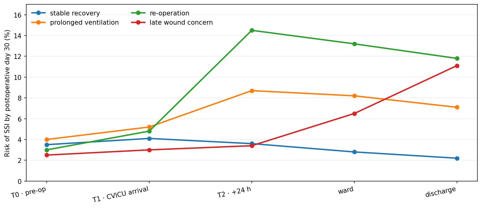
Risk can change as care unfolds

Illustrative dynamic SSI risk trajectories for four synthetic cardiac-surgery patients, updated at pre-operative, ICU transfer, ICU day one, ward transfer, and discharge landmarks.

Here, each update estimates the remaining risk of SSI by postoperative day 30 using a new information set. A fixed horizon after each landmark (e.g., risk over the next 7 days) would be a different estimand and should be labelled accordingly.

Dynamic prediction \(\rightarrow\) dynamic evaluation

At every landmark, ask:

  • who remains at risk and who has left the risk set?
  • how many events remain in the prediction horizon?
  • is discrimination stable over time?
  • are risks calibrated at that landmark and horizon?
  • how does missingness change as care changes?
  • what competing events are present?
  • would the action still be feasible and beneficial?

More updates do not guarantee more value

A 2025 comparison of static and dynamic infection-risk models found that, largely, modelling choices and competing risks affected both calibration and performance. (Gao et al. 2025)

📝 Text changes the output contract

Clinical NLP: from words to representations

A compressed history of LMs:

  1. rules, dictionaries, and hand-engineered linguistic features;
  2. bag-of-words and sparse statistical models;
  3. distributed word embeddings such as word2vec; (Mikolov et al. 2013)
  4. contextual encoders such as BERT and BioBERT; (Devlin et al. 2019; Lee et al. 2020)
  5. large language and multimodal foundation models. (Singhal et al. 2023; Moor et al. 2023)

Clinical embeddings are shaped by domain, task, and corpus. (Khattak et al. 2019)

Attention: compare, weight, combine

For each token (or event), attention asks which other items are relevant, assigns them weights, and combines the information they carry. (Vaswani et al. 2017)

Canonical multi-head pattern

Canonical multi-head attention diagram: learned linear projections feed several scaled dot-product attention heads; their outputs are concatenated and projected.

  • Query: what the current item is looking for.
  • Keys: how the other items advertise their relevance.
  • Values: the information that is mixed and passed forward.
  • Heads: several learned matching rules operating in parallel.

Source: Vaswani et al. (2017), via Wikimedia Commons; resized only. CC BY-SA 4.0.

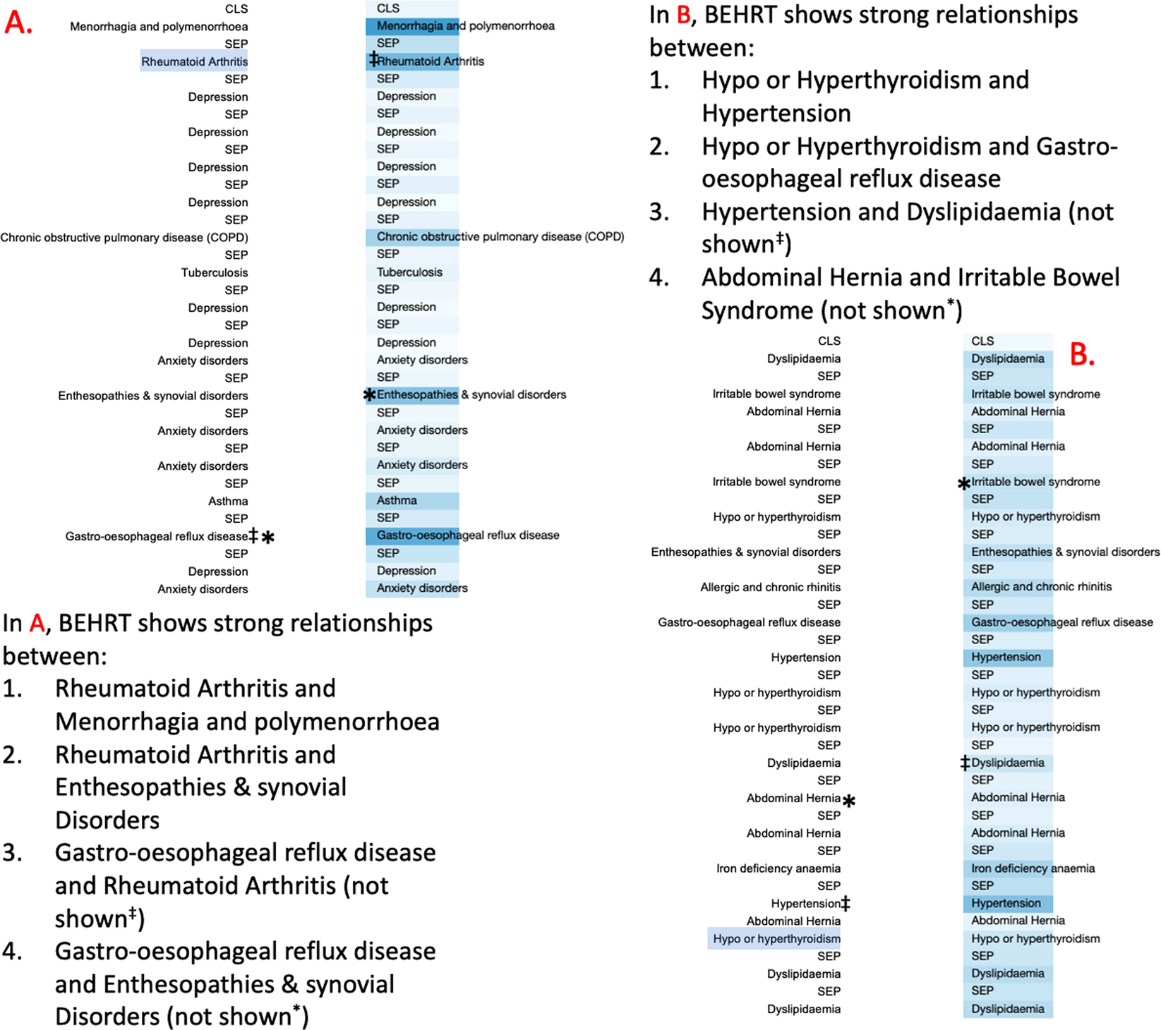
Clinical example: attention across EHR timeline

BEHRT Figure 5: two longitudinal patient histories in chronological order, with blue intensity indicating stronger final-layer attention between diagnoses.

In BEHRT, diagnoses run downward in chronological order. A diagnosis selected on the left is compared with events elsewhere in the history. The example includes a long-range association between rheumatoid arthritis and later enthesopathies or synovial disorders. (Li et al. 2020)

Source: Li et al. (2020) CC BY 4.0.

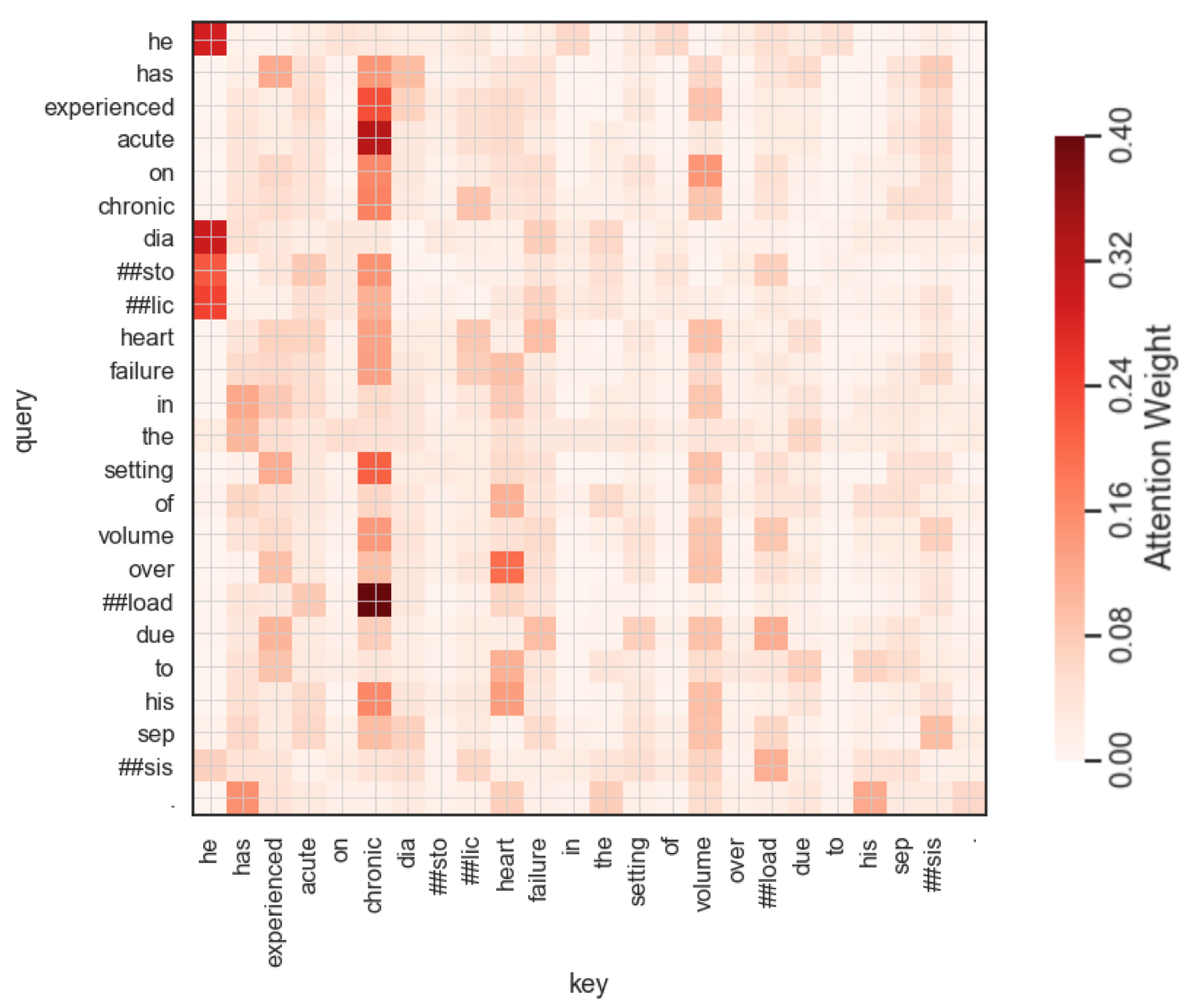
Attention weights in a clinical sentence

Each row is a query token and each column is a possible key token. A darker cell means that, in this attention head, the query placed more weight on that key while constructing its contextual representation.

ClinicalBERT token-to-token attention heatmap for an illustrative clinical sentence; darker red cells indicate larger attention weights.

One ClinicalBERT self-attention head applied to an illustrative clinical sentence. Red rendering from the nwams ClinicalBERT tutorial, based on Huang et al., Fig. 5. (nwams, n.d.; Huang, Altosaar, and Ranganath 2020)

Do not assume that attention is explanation

This heatmap shows one head, in one layer, for one sentence. A large weight does not by itself establish causality, or a faithful explanation of prediction. (Jain and Wallace 2019)

Generative versus discriminative objectives

Discriminative: learn \(P(Y\mid X)\) or a decision boundary.

Generative: learn aspects of \(P(X,Y)\), \(P(X)\), or next-token distributions that can generate new outputs.

These categories overlap in modern systems. A generative model can be used for classification; a discriminative model can sit inside a generative workflow.

Pause and discuss

In this context, how ought we evaluate: generated text quality, downstream decision quality, or patient/operational outcome?

Foundation models

Generalist medical AI aims to build reusable models that can support many tasks and adapt with little task-specific labelled data. (Moor et al. 2023; Tu et al. 2024)

Potential roles and representative systems

  • Interpret multiple modalities: Med-PaLM M combines language with information such as medical images, genomics, and structured clinical data. (Tu et al. 2024)

  • Conduct diagnostic dialogue: AMIE was developed for conversational history-taking, diagnostic reasoning, and communication. (Tu et al. 2025; McDuff et al. 2025)

  • Use tools and execute workflows: MedAgentBench evaluates LLM agents that retrieve information and perform multi-step tasks through a FHIR-compatible EHR environment. (Jiang et al. 2025)

Generation changes the evaluation contract

For generated output, “is the class correct?” is no longer enough. Evaluation may need to examine factuality, coverage, clinical reasoning, safety, bias and equity, confidence, naturalness, privacy, et c.

MEDIC, e.g., combines different tasks and metrics across five dimensions of clinical competence; others add user-centred, trustworthiness, privacy, empathy, and operational measures. No single score establishes that a generative system is clinically useful. (Kanithi et al. 2026; Abbasian et al. 2024)

A benchmark is not a workflow

benchmark mistake

A model can perform well on exams or simulated consultations yet fail to improve a clinician–AI team.

This is especially relevant for results on AIRO-Sim.

In a randomized trial of 50 physicians, access to an LLM did not significantly improve diagnostic reasoning compared with conventional resources, despite strong standalone model performance. (Goh et al. 2024)

Evidence

Human–AI performance depends on interface, human psychology, task allocation, training, time, trust, and how disagreements are resolved.

5 · From prediction to clinical action and audit

High risk \(\neq\) high treatment benefit

target mistake

A prognostic model estimates what may happen under the patterns in its development data.

A treatment decision requires a comparison between alternative actions. Let \(Y^a\) denote the adverse outcome that would occur under action \(a\), with \(a_0\) as the comparator. For patients with characteristics \(x\),

\[ B(x) = P(Y^{a_0}=1\mid X=x) - P(Y^{a}=1\mid X=x). \]

A positive \(B(x)\) means that action \(a\) is expected to reduce absolute outcome risk relative to the comparator. This is an expected conditional benefit: both potential outcomes cannot be observed for the same patient. (Kent, Steyerberg, and Klaveren 2018; Geloven et al. 2020)

A high-risk patient may have:

  • little modifiable risk;
  • a poor response to the available intervention;
  • substantial treatment-related harm or burden.

A moderate-risk patient may have:

  • a large preventable component of risk;
  • a strong response to an effective intervention;
  • little treatment-related harm or burden.

High risk \(\neq\) high treatment benefit

Baseline risk can still help predict absolute benefit when relative treatment effects and harms are reasonably stable, but risk and benefit are not “two sides of the same coin.”

If a predictor prompts effective treatment, the resulting prevention of outcomes can make that predictor appear less prognostic in historical data. This treatment paradox can cause an ordinary prognostic model to underestimate risk under no treatment. (Sperrin et al. 2018; Geloven et al. 2020)

A risk score is not a treatment rule

Before recommending an action, specify the intervention, comparator, expected benefit, harms and burden then ask whether model-guided decisions improve net benefit relative to usual care.

Interpretability: choose the question first

Possible questions:

  • Why did this linear score increase?
  • Which observations most influenced this prediction?
  • What global patterns has the model learned?
  • Is the model relying on a shortcut?
  • What would need to change for the prediction to differ?
  • Can a clinician verify the evidence source?
  • Does the explanation improve decisions or merely confidence?

Risk

An attractive explanation can be unstable, incomplete, or persuasive without being faithful. (Ghassemi, Oakden-Rayner, and Beam 2021b)

Error autopsy

First, not every problem is linear (Rudin 2019). A suspiciously strong model might be using:

  • postoperative antibiotics or cultures;
  • a diagnosis code entered after outcome recognition;
  • repeated notes from the same encounter across splits;
  • site or year as a proxy for the label;
  • missingness revealing a ward or service;
  • a device or documentation transition;
  • follow-up intensity rather than true event occurrence.

Pause and discuss

For each top feature, ask: could this exist, in this form, at the intended prediction time in a new patient?

Activity · red-team a plausible SSI study

Proposed claim: “At the end of surgery, our model can identify patients at high risk of SSI within 30 days so that enhanced wound follow-up can be targeted.”

Available data: 2,400 surgeries over 12 years; 72 recorded SSIs (3%); 30 candidate registry variables; repeated operations for some patients; and a registry redesign after year 6.

The proposed analysis

  1. Randomly split surgery rows 80/20 into development and test sets.
  2. Retain all 30 candidate fields, including postoperative variables that are strongly associated with SSI.
  3. In the development set, impute, standardize, and apply SMOTE once; then use five-fold cross-validation to tune logistic regression, random forest, XGBoost, and a neural network.
  4. Select the model with the highest cross-validated AUROC.
  5. On the test set, choose the threshold that maximizes F1 and report AUROC, accuracy, and F1.
  6. Report subgroup AUROCs by sex, age quartile, and procedure type.
  7. Recommend an alert for patients classified as “high risk.”

Your role: independent review panel

⏲️ 15 minutes: Would you approve this study as written?

Identify the three most consequential threats to a credible result. For each one, explain why it matters and propose the smallest repair that would make the first experiment defensible.

Practical standards for Health+AI work

A strong project will ideally lean into aspects of machine learning (e.g., modelling itself or its use) but also into aspects of reproducibility so another professional can reproduce and evaluate your work.

Make the evidence auditable

  • define the population, time, outcome, and intended use;
  • justify model complexity against the information available;
  • preserve an untouched evaluation set;
  • report calibration, uncertainty, event counts, and failure modes.

Make the limits actionable

  • separate prediction from intervention benefit;
  • name the workflow, burden, and people affected;
  • document what the study cannot establish;
  • leave an audit trail that supports review and improvement.

Ambition with discipline

Build with curiosity, confidence, and ambition, but keep every claim proportional to the evidence! (Collins, Moons, et al. 2024; Moons et al. 2025; Vasey et al. 2022; Lekadir et al. 2025)

References

Abbasian, Mahyar, Elahe Khatibi, Iman Azimi, David Oniani, Zahra Shakeri Hossein Abad, Alexander Thieme, Ram Sriram, et al. 2024. “Foundation Metrics for Evaluating Effectiveness of Healthcare Conversations Powered by Generative AI.” Npj Digital Medicine 7 (1): 82. https://doi.org/10.1038/s41746-024-01074-z.
Adebayo, Julius, Justin Gilmer, Michael Muelly, Ian Goodfellow, Moritz Hardt, and Been Kim. 2018. “Sanity Checks for Saliency Maps.” In Advances in Neural Information Processing Systems, 31:9525–36.
Afshar, Majid, Mary Ryan Baumann, et al. 2025. “A Pragmatic Randomized Controlled Trial of Ambient Artificial Intelligence to Improve Health Practitioner Well-Being.” NEJM AI 2 (12). https://doi.org/10.1056/AIoa2500945.
Beede, Emma, Elizabeth Baylor, Fred Hersch, Anna Iurchenko, Lauren Wilcox, Paisan Ruamviboonsuk, and Laura M. Vardoulakis. 2020. “A Human-Centered Evaluation of a Deep Learning System Deployed in Clinics for the Detection of Diabetic Retinopathy.” In Proceedings of the 2020 CHI Conference on Human Factors in Computing Systems, 1–12. https://doi.org/10.1145/3313831.3376718.
Caruana, Rich, Yin Lou, Johannes Gehrke, Paul Koch, Marc Sturm, and Noémie Elhadad. 2015. “Intelligible Models for HealthCare: Predicting Pneumonia Risk and Hospital 30-Day Readmission.” In Proceedings of the 21th ACM SIGKDD International Conference on Knowledge Discovery and Data Mining, 1721–30. https://doi.org/10.1145/2783258.2788613.
Catling, Finneas J. R., and Anthony H. Wolff. 2020. “Temporal Convolutional Networks Allow Early Prediction of Events in Critical Care.” Journal of the American Medical Informatics Association 27 (3): 355–65. https://doi.org/10.1093/jamia/ocz205.
Chawla, Nitesh V., Kevin W. Bowyer, Lawrence O. Hall, and W. Philip Kegelmeyer. 2002. “SMOTE: Synthetic Minority over-Sampling Technique.” Journal of Artificial Intelligence Research 16: 321–57. https://doi.org/10.1613/jair.953.
Che, Zhengping, Sanjay Purushotham, Kyunghyun Cho, David Sontag, and Yan Liu. 2018. “Recurrent Neural Networks for Multivariate Time Series with Missing Values.” Scientific Reports 8 (1): 6085. https://doi.org/10.1038/s41598-018-24271-9.
Collins, Gary S., Paul Dhiman, Jia Ma, Michael Schlussel, Luke Archer, Ben Van Calster, et al. 2024. “Evaluation of Clinical Prediction Models (Part 1): From Development to External Validation.” BMJ 384: e074819. https://doi.org/10.1136/bmj-2023-074819.
Collins, Gary S., Karel G. M. Moons, Paul Dhiman, Richard D. Riley, Andrew L. Beam, Ben Van Calster, et al. 2024. “TRIPOD+AI Statement: Updated Guidance for Reporting Clinical Prediction Models That Use Regression or Machine Learning Methods.” BMJ 385: e078378. https://doi.org/10.1136/bmj-2023-078378.
Devlin, Jacob, Ming-Wei Chang, Kenton Lee, and Kristina Toutanova. 2019. “BERT: Pre-Training of Deep Bidirectional Transformers for Language Understanding.” In Proceedings of NAACL-HLT, 4171–86. https://doi.org/10.18653/v1/N19-1423.
Efthimiou, Orestis, Myeong Soo Seo, Katerina Chalkou, Thomas P. A. Debray, Matthias Egger, and Georgia Salanti. 2024. “Developing Clinical Prediction Models: A Step-by-Step Guide.” BMJ 386: e078276. https://doi.org/10.1136/bmj-2023-078276.
Esteva, Andre, Brett Kuprel, Roberto A. Novoa, Justin Ko, Susan M. Swetter, Helen M. Blau, and Sebastian Thrun. 2017. “Dermatologist-Level Classification of Skin Cancer with Deep Neural Networks.” Nature 542: 115–18. https://doi.org/10.1038/nature21056.
Esteva, Andre, Alexandre Robicquet, Bharath Ramsundar, Volodymyr Kuleshov, Mark DePristo, Katherine Chou, Claire Cui, Greg Corrado, Sebastian Thrun, and Jeff Dean. 2019. “A Guide to Deep Learning in Healthcare.” Nature Medicine 25 (1): 24–29. https://doi.org/10.1038/s41591-018-0316-z.
Finlayson, Samuel G., Adarsh Subbaswamy, Karandeep Singh, John Bowers, Alexander Kupke, Jonathan Zittrain, et al. 2021. “The Clinician and Dataset Shift in Artificial Intelligence.” New England Journal of Medicine 385: 283–86. https://doi.org/10.1056/NEJMc2104626.
Futoma, Joseph, Sanjay Hariharan, and Katherine Heller. 2017. “Learning to Detect Sepsis with a Multitask Gaussian Process RNN Classifier.” In Proceedings of Machine Learning for Healthcare, 68:117–35. Proceedings of Machine Learning Research. https://proceedings.mlr.press/v68/futoma17a.html.
Gao, Shan, Elena Albu, Hein Putter, Pieter Stijnen, Frank E. Rademakers, Veerle Cossey, Yves Debaveye, Christel Janssens, Ben Van Calster, and Laure Wynants. 2025. “A Comparison of Modeling Approaches for Static and Dynamic Prediction of Central-Line Bloodstream Infections Using Electronic Health Records (Part 1): Regression Models.” Diagnostic and Prognostic Research 9: 20. https://doi.org/10.1186/s41512-025-00199-3.
Geloven, Nan van, Sonja A. Swanson, Chava L. Ramspek, Kim Luijken, Merel van Diepen, Tim P. Morris, Rolf H. H. Groenwold, Hans C. van Houwelingen, Hein Putter, and Saskia le Cessie. 2020. “Prediction Meets Causal Inference: The Role of Treatment in Clinical Prediction Models.” European Journal of Epidemiology 35 (7): 619–30. https://doi.org/10.1007/s10654-020-00636-1.
Ghassemi, Marzyeh, Luke Oakden-Rayner, and Andrew L. Beam. 2021a. “The False Hope of Current Approaches to Explainable Artificial Intelligence in Health Care.” The Lancet Digital Health 3 (11): e745–50. https://doi.org/10.1016/S2589-7500(21)00208-9.
———. 2021b. “The False Hope of Current Approaches to Explainable Artificial Intelligence in Health Care.” The Lancet Digital Health 3 (11): e745–50. https://doi.org/10.1016/S2589-7500(21)00208-9.
Ghassemi, Marzyeh, Marco A. F. Pimentel, Tristan Naumann, Thomas Brennan, David A. Clifton, Peter Szolovits, and Mengling Feng. 2015. “A Multivariate Timeseries Modeling Approach to Severity of Illness Assessment and Forecasting in ICU with Sparse, Heterogeneous Clinical Data.” Proceedings of the AAAI Conference on Artificial Intelligence 29 (1): 446–53. https://doi.org/10.1609/aaai.v29i1.9209.
Gichoya, Judy Wawira, Imon Banerjee, Ananth Reddy Bhimireddy, John L. Burns, Leo Anthony Celi, Li-Ching Chen, Ramon Correa, et al. 2022. “AI Recognition of Patient Race in Medical Imaging: A Modelling Study.” The Lancet Digital Health 4 (6): e406–14. https://doi.org/10.1016/S2589-7500(22)00063-2.
Goh, Ethan, Robert Gallo, Jonathan Hom, et al. 2024. “Large Language Model Influence on Diagnostic Reasoning: A Randomized Clinical Trial.” JAMA Network Open 7 (10): e2440969. https://doi.org/10.1001/jamanetworkopen.2024.40969.
Goorbergh, Ruben van den, Maarten van Smeden, Dirk Timmerman, and Ben Van Calster. 2022. “The Harm of Class Imbalance Corrections for Risk Prediction Models: Illustration and Simulation Using Logistic Regression.” Journal of the American Medical Informatics Association 29 (9): 1525–34. https://doi.org/10.1093/jamia/ocac093.
Gulshan, Varun, Lily Peng, Marc Coram, Martin C. Stumpe, Derek Wu, Arunachalam Narayanaswamy, et al. 2016. “Development and Validation of a Deep Learning Algorithm for Detection of Diabetic Retinopathy in Retinal Fundus Photographs.” JAMA 316 (22): 2402–10. https://doi.org/10.1001/jama.2016.17216.
Huang, Kexin, Jaan Altosaar, and Rajesh Ranganath. 2020. “ClinicalBERT: Modeling Clinical Notes and Predicting Hospital Readmission.” In ACM Conference on Health, Inference, and Learning, Workshop Track. Toronto, Ontario, Canada. https://doi.org/10.48550/arXiv.1904.05342.
Jain, Sarthak, and Byron C. Wallace. 2019. “Attention Is Not Explanation.” In Proceedings of the 2019 Conference of the North American Chapter of the Association for Computational Linguistics: Human Language Technologies, Volume 1 (Long and Short Papers), 3543–56. Minneapolis, Minnesota: Association for Computational Linguistics. https://doi.org/10.18653/v1/N19-1357.
Jiang, Yixing, Kameron C. Black, Gloria Geng, Danny Park, James Zou, Andrew Y. Ng, and Jonathan H. Chen. 2025. “MedAgentBench: A Virtual EHR Environment to Benchmark Medical LLM Agents.” NEJM AI 2 (9). https://doi.org/10.1056/AIdbp2500144.
Kanithi, Praveenkumar, Clément Christophe, Marco A. F. Pimentel, Tathagata Raha, Prateek Munjal, Nada Saadi, Hamza A. Javed, et al. 2026. “MEDIC: Comprehensive Evaluation of Leading Indicators for LLM Safety and Utility in Clinical Applications.” Transactions on Machine Learning Research, June. https://openreview.net/forum?id=pDQe9Icwb6.
Kapoor, Sayash, Emily M. Cantrell, Kenny Peng, Tuan H. Pham, Christopher A. Bail, Odd Erik Gundersen, et al. 2024. “REFORMS: Consensus-Based Recommendations for Machine-Learning-Based Science.” Science Advances 10 (18): eadk3452. https://doi.org/10.1126/sciadv.adk3452.
Kelly, Christopher J., Alan Karthikesalingam, Mustafa Suleyman, Greg Corrado, and Dominic King. 2019. “Key Challenges for Delivering Clinical Impact with Artificial Intelligence.” BMC Medicine 17: 195. https://doi.org/10.1186/s12916-019-1426-2.
Kent, David M., Ewout W. Steyerberg, and David van Klaveren. 2018. “Personalized Evidence Based Medicine: Predictive Approaches to Heterogeneous Treatment Effects.” BMJ 363: k4245. https://doi.org/10.1136/bmj.k4245.
Khattak, Faiza K., Serena Jeblee, Chloé Pou-Prom, Mohamed Abdalla, Christopher Meaney, and Frank Rudzicz. 2019. “A Survey of Word Embeddings for Clinical Text.” Journal of Biomedical Informatics 100: 103057. https://doi.org/10.1016/j.jbi.2019.103057.
Lee, Jinhyuk, Wonjin Yoon, Sungdong Kim, Donghyeon Kim, Sunkyu Kim, Chan Ho So, and Jaewoo Kang. 2020. “BioBERT: A Pre-Trained Biomedical Language Representation Model for Biomedical Text Mining.” Bioinformatics 36 (4): 1234–40. https://doi.org/10.1093/bioinformatics/btz682.
Lehman, Eric, and Alistair Johnson. 2023. “Clinical-T5: Large Language Models Built Using MIMIC Clinical Text.” PhysioNet. https://doi.org/10.13026/rj8x-v335.
Lehman, Li-Wei H., Mohammad Ghassemi, Jasper Snoek, and Shamim Nemati. 2015. “Patient Prognosis from Vital Sign Time Series: Combining Convolutional Neural Networks with a Dynamical Systems Approach.” Computing in Cardiology 42: 1069–72. https://doi.org/10.1109/CIC.2015.7411099.
Lekadir, Karim, Alejandro F. Frangi, Antonio R. Porras, Ben Glocker, et al. 2025. “FUTURE-AI: International Consensus Guideline for Trustworthy and Deployable Artificial Intelligence in Healthcare.” BMJ 388: e081554. https://doi.org/10.1136/bmj-2024-081554.
Li, Yikuan, Shishir Rao, José Roberto Ayala Solares, Abdelaali Hassaine, Rema Ramakrishnan, Dexter Canoy, Yajie Zhu, Kazem Rahimi, and Gholamreza Salimi-Khorshidi. 2020. “BEHRT: Transformer for Electronic Health Records.” Scientific Reports 10 (1): 7155. https://doi.org/10.1038/s41598-020-62922-y.
Lotter, William, Alexandra R. Diab, Benjamin Haslam, et al. 2024. “Acquisition Parameters Influence AI Recognition of Race in Chest x-Rays and Mitigating These Factors Reduces Underdiagnosis Bias.” Nature Communications 15. https://doi.org/10.1038/s41467-024-52003-3.
McDuff, Daniel, Mike Schaekermann, Tao Tu, et al. 2025. “Towards Accurate Differential Diagnosis with Large Language Models.” Nature 642: 451–57. https://doi.org/10.1038/s41586-025-08869-4.
Mikolov, Tomas, Ilya Sutskever, Kai Chen, Greg S. Corrado, and Jeffrey Dean. 2013. “Distributed Representations of Words and Phrases and Their Compositionality.” In Advances in Neural Information Processing Systems. Vol. 26. https://proceedings.neurips.cc/paper/2013/hash/9aa42b31882ec039965f3c4923ce901b-Abstract.html.
Moons, Karel G. M., Robert F. Wolff, Richard D. Riley, Penny F. Whiting, Marie Westwood, Gary S. Collins, et al. 2025. “PROBAST+AI: An Updated Quality, Risk of Bias, and Applicability Assessment Tool for Prediction Models Using Regression or Artificial Intelligence Methods.” BMJ 388: e082505. https://doi.org/10.1136/bmj-2024-082505.
Moor, Michael, Oishi Banerjee, Zahra Shakeri Hossein Abad, Harlan M. Krumholz, Jure Leskovec, Eric J. Topol, and Pranav Rajpurkar. 2023. “Foundation Models for Generalist Medical Artificial Intelligence.” Nature 616: 259–65. https://doi.org/10.1038/s41586-023-05881-4.
nwams. n.d. “ClinicalBERT: Using Deep Learning Transformer Model to Predict Hospital Readmission.” GitHub repository and tutorial. https://github.com/nwams/ClinicalBERT-Deep-Learning--Predicting-Hospital-Readmission-Using-Transformer.
Ovadia, Yaniv, Emily Fertig, Jie Ren, Zachary Nado, D. Sculley, Sebastian Nowozin, Joshua Dillon, Balaji Lakshminarayanan, and Jasper Snoek. 2019. “Can You Trust Your Model’s Uncertainty? Evaluating Predictive Uncertainty Under Dataset Shift.” In Advances in Neural Information Processing Systems, 32:13991–4002.
Riley, Richard D., Luke Archer, Kym I. E. Snell, Joie Ensor, Paul Dhiman, Glen P. Martin, et al. 2024. “Evaluation of Clinical Prediction Models (Part 2): How to Undertake an External Validation Study.” BMJ 384: e074820. https://doi.org/10.1136/bmj-2023-074820.
Riley, Richard D., Thomas P. A. Debray, Gary S. Collins, Luke Archer, Joie Ensor, Maarten van Smeden, et al. 2024. “Evaluation of Clinical Prediction Models (Part 3): Calculating the Sample Size Required for an External Validation Study.” BMJ 384: e074821. https://doi.org/10.1136/bmj-2023-074821.
Riley, Richard D., Kym I. E. Snell, Luke Archer, Joie Ensor, Gary S. Collins, et al. 2025. “Uncertainty of Risk Estimates from Clinical Prediction Models.” BMJ 388: e080749. https://doi.org/10.1136/bmj-2024-080749.
Rudin, Cynthia. 2019. “Stop Explaining Black Box Machine Learning Models for High Stakes Decisions and Use Interpretable Models Instead.” Nature Machine Intelligence 1: 206–15. https://doi.org/10.1038/s42256-019-0048-x.
Sendak, Mark P., Joshua D’Arcy, Sehj Kashyap, Michael Gao, Marshall Nichols, Kristin Corey, William Ratliff, and Suresh Balu. 2020. “A Path for Translation of Machine Learning Products into Healthcare Delivery.” EMJ Innovation. https://doi.org/10.33590/emjinnov/19-00172.
Seth, Puneet, Romina Carretas, and Frank Rudzicz. 2024. “The Utility and Implications of Ambient Scribes in Primary Care.” JMIR AI 3 (October): e57673. https://doi.org/10.2196/57673.
Seyyed-Kalantari, Laleh, Haoran Zhang, Matthew B. A. McDermott, Irene Y. Chen, and Marzyeh Ghassemi. 2021. “Underdiagnosis Bias of Artificial Intelligence Algorithms Applied to Chest Radiographs in Under-Served Patient Populations.” Nature Medicine 27: 2176–82. https://doi.org/10.1038/s41591-021-01595-0.
Singhal, Karan, Shekoofeh Azizi, Tao Tu, S. Sara Mahdavi, Jason Wei, Hyung Won Chung, et al. 2023. “Large Language Models Encode Clinical Knowledge.” Nature 620: 172–80. https://doi.org/10.1038/s41586-023-06291-2.
Sperrin, Matthew, Glen P. Martin, Alexander Pate, Tjeerd van Staa, Niels Peek, and Iain Buchan. 2018. “Using Marginal Structural Models to Adjust for Treatment Drop-in When Developing Clinical Prediction Models.” Statistics in Medicine 37 (28): 4142–54. https://doi.org/10.1002/sim.7913.
Stevens, Richard J., and Katrina K. Poppe. 2020. “Validation of Clinical Prediction Models: What Does the ‘Calibration Slope’ Really Measure?” Journal of Clinical Epidemiology 118 (February): 93–99. https://doi.org/10.1016/j.jclinepi.2019.09.016.
Tu, Tao, Shekoofeh Azizi, Danny Driess, Mike Schaekermann, Mohamed Amin, Pi-Chuan Chang, et al. 2024. “Towards Generalist Biomedical AI.” NEJM AI 1: AIoa2300138. https://doi.org/10.1056/AIoa2300138.
Tu, Tao, Mike Schaekermann, Arvind Palepu, et al. 2025. “Towards Conversational Diagnostic Artificial Intelligence.” Nature 642: 442–50. https://doi.org/10.1038/s41586-025-08866-7.
Van Calster, Ben, Daan Nieboer, Yvonne Vergouwe, Bavo De Cock, Michael J. Pencina, and Ewout W. Steyerberg. 2016. “A Calibration Hierarchy for Risk Models Was Defined: From Utopia to Empirical Data.” Journal of Clinical Epidemiology 74: 167–76. https://doi.org/10.1016/j.jclinepi.2015.12.005.
Varoquaux, Gaël, and Veronika Cheplygina. 2022. “Machine Learning for Medical Imaging: Methodological Failures and Recommendations for the Future.” Npj Digital Medicine 5: 48. https://doi.org/10.1038/s41746-022-00592-y.
Vasey, Baptiste, Myura Nagendran, Bruce Campbell, David A. Clifton, Gary S. Collins, Spiros Denaxas, et al. 2022. “Reporting Guideline for the Early-Stage Clinical Evaluation of Decision Support Systems Driven by Artificial Intelligence: DECIDE-AI.” Nature Medicine 28: 924–33. https://doi.org/10.1038/s41591-022-01772-9.
Vaswani, Ashish, Noam Shazeer, Niki Parmar, Jakob Uszkoreit, Llion Jones, Aidan N. Gomez, Łukasz Kaiser, and Illia Polosukhin. 2017. “Attention Is All You Need.” In Advances in Neural Information Processing Systems. Vol. 30. https://proceedings.neurips.cc/paper/2017/hash/3f5ee243547dee91fbd053c1c4a845aa-Abstract.html.
Vickers, Andrew J., Ben Van Calster, and Ewout W. Steyerberg. 2016. “Net Benefit Approaches to the Evaluation of Prediction Models, Molecular Markers, and Diagnostic Tests.” BMJ 352: i6. https://doi.org/10.1136/bmj.i6.
Wiens, Jenna, Suchi Saria, Mark Sendak, Marzyeh Ghassemi, Vincent X. Liu, Finale Doshi-Velez, Kenneth Jung, et al. 2019. “Do No Harm: A Roadmap for Responsible Machine Learning for Health Care.” Nature Medicine 25 (9): 1337–40. https://doi.org/10.1038/s41591-019-0548-6.
Yang, Xi, Aokun Chen, Nima PourNejatian, Hoo Chang Shin, Kaleb E. Smith, Christopher Parisien, Colin Compas, et al. 2022. “A Large Language Model for Electronic Health Records.” Npj Digital Medicine 5 (1): 194. https://doi.org/10.1038/s41746-022-00742-2.
Zakka, Cyril, Rohan Shad, Akash Chaurasia, Alex R. Dalal, Jennifer L. Kim, Michael Moor, Robyn Fong, et al. 2024. “Almanac: Retrieval-Augmented Language Models for Clinical Medicine.” NEJM AI 1 (2). https://doi.org/10.1056/AIoa2300068.
Zech, John R., Marcus A. Badgeley, Manway Liu, Anthony B. Costa, Joseph J. Titano, and Eric Karl Oermann. 2018. “Variable Generalization Performance of a Deep Learning Model to Detect Pneumonia in Chest Radiographs: A Cross-Sectional Study.” PLOS Medicine 15 (11): e1002683. https://doi.org/10.1371/journal.pmed.1002683.