flowchart LR
  C[Care and workflow] --> M[Measurement]
  M --> R[Clinical record]
  R --> T[Analysis table]
  T --> P[Model or estimate]
  P --> E[Evidence and uncertainty]
  E --> D[Decision and action]
Operationalized Machine Learning in Healthcare
Lec 2: Clinical data science foundations: from care to evidence
Frank Rudzicz
DGIN 5401 · Dalhousie University
How care becomes data
Clinical data science:
data → evidence → decision
Practical
- begin with the decision;
- define success and a baseline;
- design evaluation before inspecting the test set;
- document assumptions and limits.
Clinical and scientific
- ask who or what generated each value;
- respect timing, missingness, workflow, and incentives;
- make a claim that could fail;
- connect errors to people, workload, and harm.
Every transformation changes what the data can mean and what claim the result can support.
How a patient becomes a datum
flowchart LR
  A[Patient and circumstances] --> B[Access and care-seeking]
  B --> C[Clinical workflow and measurement]
  C --> D[Documentation and coding]
flowchart LR
  D[Documentation and coding] --> E[Database extraction]
  E --> F[Cohort and label construction]
  F --> G[Training table]
  G --> H[Model]
At each transition: selection, measurement, missingness, and institutional policy can alter what is visible to the modeller. (Agniel, Kohane, and Weber 2018; Suresh and Guttag 2021)
Health data are gathered for care
The registry and EHR were not created to test your hypothesis.
- measurements occur at different rates;
- tests are ordered because someone happened to feel concerned;
- documentation reflects roles and incentives;
- codes may support billing, surveillance, or reporting;
- absent data may indicate “not done,” “not needed,” or “not captured”;
- follow-up depends on where patients receive care.
Data principle
The data-generation process is part of the model, even if you didn’t mean it to be.
The measurement can be biased before ML
Pulse oximetry is an input to care and to many predictive pipelines.
In one hospital cohort, when pulse oximetry displayed 92–96%, occult hypoxemia was present in 11.7% of Black patients and 3.6% of White patients
- the disparity was also present in a large multicentre cohort. (Sjoding et al. 2020)
A model trained on sensor values can inherit measurement error, treatment differences caused by that error, and labels produced downstream.
Audit the instrument
Before asking whether the model is ‘fair’, ask whether the measurement process is valid across the people and environments in which it will be used.
A multi-modal care pathway
Across one episode, available data may include:
- demographics, history, comorbidities, medications;
- pre-operative labs and imaging;
- procedure details and device use;
- continuous intraoperative waveforms and events;
- ICU/ward vitals, labs, medications, supports, and mobility;
- clinical notes and wound descriptions;
- discharge plans, calls, photographs, and follow-up outcomes.
Public resources such as 🔗 MIMIC and 🔗 PhysioNet illustrate some breadth and complexity of clinical data, though they can also be limited. (Johnson et al. 2023; Goldberger et al. 2000)
Structured codes are not self-explanatory
Common terminologies include:
- 🔗 ICD for diagnoses and conditions;
- procedure classifications and local surgical codes;
- 🔗 LOINC for laboratory observations;
- 🔗 SNOMED CT for clinical concepts;
- medication identifiers such as DIN, NDC, or RxNorm;
- local device, location, and workflow codes.
Check version, granularity, mapping, and whether a code records a true event, a rule-out diagnosis, a billing choice, or a documentation habit.
Clinical text adds context—and ambiguity
Notes may reveal:
- uncertainty, differential diagnosis, and rationale;
- symptoms and findings absent from structured fields;
- negation, temporality, experiencer, and severity;
- care plans and social context;
- early wound concerns or follow-up communication.
(Ford et al. 2016; Harkema et al. 2009; Bucher et al. 2020)
They also contain templates, copied text, shorthand, inconsistent terminology, and information written after the prediction cut-off. (Rule et al. 2021; Davis et al. 2024)
Naturalistic note fragments
Pre-operative consult
Patient reports independent mobility at baseline. HbA1c has improved, but home glucose remains variable. No active skin lesions. Discussed sternal precautions and expected recovery.
Operative note
Combined CABG and valve procedure. Prolonged bypass due to difficult exposure. Rewarming uncomplicated. No gross contamination. Skin closed at 18:42.
Ward nursing note
Incision dry at morning assessment. Later noted mild inferior erythema without drainage. Patient afebrile; pain increased with cough. Team notified.
Follow-up message
Patient sent photograph through portal. Reports new drainage and fatigue since yesterday. Community prescription started; asked to attend urgent review.
Pause and discuss
Which fragment is available at each proposed prediction time? Which terms require context, negation, or temporal interpretation?
Clinical tables have several identities
A “patient row” may actually represent a patient, admission, procedure, specimen, device episode, note, or measurement.
| Key | Possible unit |
|---|---|
patient_id |
person |
admission_id |
hospitalization |
surgery_id |
operation |
specimen_id |
microbiology sample |
note_id |
document |
measurement_id |
one recorded value |
Join audit
Before joining, state the expected relationship: one-to-one, one-to-many, or many-to-many. Then verify row counts and duplicate keys. Accidental row multiplication can manufacture sample size and leakage.
Repeated clinical data: long versus wide
Long form
| surgery_id | time | creatinine |
|---|---|---|
| A01 | pre-op | 82 |
| A01 | ICU+6h | 104 |
| A01 | ICU+24h | 131 |
Natural for irregular measurements and trajectories.
Wide form
| surgery_id | cr_pre | cr_6h | cr_24h |
|---|---|---|---|
| A01 | 82 | 104 | 131 |
Convenient for some models, but requires explicit windows and missing-value rules.
The transformation from long to wide quietly chooses which measurements count, how they are summarized, and what time means.
One value can have three clocks
For a laboratory result, distinguish:
specimen collected→result available→result entered or corrected
- measurement time: when physiology was sampled;
- availability time: when the model or clinician could have known it;
- record time: when the database stored or updated it.
Prediction-time rule
Features must be filtered by the time they were available, not merely by the date attached to the observation.
The same distinction applies to notes, diagnoses, orders, and discharge summaries.
AIRO-Sim prediction snapshots
| Snapshot | When is the prediction made? | Information available | Course role |
|---|---|---|---|
| T0 | Before the operation begins | Preoperative history, status, labs, planned procedure, and preoperative note | Required shared backbone |
| T1 | At CVICU arrival | T0 plus performed procedure, intraoperative support and events, and handoff note | Optional dynamic update |
| T2 | Approximately 24 h after surgery | T0/T1 plus early postoperative events and available POD1 note | Optional landmark analysis |
An information boundary, not just a timestamp
A predictor may enter a model only if it could have been available to the intended user by that snapshot.
The snapshot does not define the outcome horizon. At each later landmark, specify who remains at risk and what future outcome is still being predicted.
Not prediction features
Discharge and outcome-only information cannot enter T0 or T1. Identifiers, split labels, and synthetic-era fields are for linkage, audit, or evaluation.
Values need context, units, and provenance
Common failure modes include:
- 🔗 creatinine in \(\mu\mathrm{mol/L}\) mixed with \(\mathrm{mg/dL}\);
- weight in pounds mixed with kilograms;
- a default zero used for “not measured”;
- reference ranges that vary by laboratory;
- repeated extracts of the same event;
- corrected values treated as independent measurements;
- copied-forward documentation;
- version changes in devices, forms, or code systems.
A useful audit table
For every important variable, record: meaning, unit, valid range, source system, timestamp semantics, missing-value codes, and known version changes.
A clinical supervised-learning table
| surgery_id | age | diabetes | bypass_minutes | preop_hgb | SSI_30d |
|---|---|---|---|---|---|
| A001 | 67 | 1 | 121 | 119 | 0 |
| A002 | 54 | 0 | 88 | 137 | 0 |
| A003 | 73 | 1 | 176 | 108 | 1 |
| … | … | … | … | … | … |
rows     = surgeries / observations
columns  = measurements, codes, or derived features
X        = feature matrix
y        = target / outcome
f(X)     = model scores or predictions
ŷ        = prediction
loss     = training objective we aim to minimize (e.g., error)
metric   = evaluation summary (e.g., accuracy)
Four questions before code
What is the row unit? Which columns exist by the prediction time? Which columns are actions or consequences?
How data become a study
Data-quality dimensions
A practical audit asks about:
- Accuracy — does the value represent the intended concept?
- Precision — is the resolution sufficient?
- Completeness — what is absent, and for whom?
- Consistency — do formats, units, and definitions align?
- Timeliness — was the value available at the decision time?
- Believability — is the value plausible given the workflow?
- Interpretability — can analysts and users understand it?
A more recent systematic framework organizes data-quality dimensions for trustworthy medical AI. (Schwabe et al. 2024)
Dirty data: six recurring forms
- inconsistent types:
M,male,1; - inconsistent values or units: mg versus g, minutes versus hours;
- missing fields or sentinel values such as
-1; - outliers and impossible combinations;
- recording errors, duplicates, and noisy labels;
- inconsistent concept granularity, such as specific versus broad codes.
Pause and discuss
Which problems can be detected mechanically? Which require domain knowledge or source-system review?
Missingness can be accidentally predictive
Let \(M_j=\mathbb{1}(X_j\text{ was observed})\). In clinical data, \(M_j\) may encode:
Patient and care process
- clinician concern & decision to test;
- severity and intensity of monitoring;
- transfer, discharge, or care received elsewhere.
Local measurement system
- ward, service, or site workflow;
- device, interface, or registry availability;
- staffing, (documentation) policy.
The model can therefore predict from who gets measured, when, and where, not only from the measured value. Test-ordering patterns can be as predictive as, or more predictive than, the test results themselves. (Agniel, Kohane, and Weber 2018; Groenwold 2020)
Useful internally does not mean transportable
A missingness indicator may improve internal validation while learning a local observation policy. If ordering or recording practices change, \(P(Y\mid M_j)\) can change and model performance can deteriorate. (Groenwold 2020; Nestor et al. 2019)
Audit: report missingness by outcome, service or site, era, and subgroup; compare models with and without missingness features; validate temporally and externally.
Label quality and inter-rater agreement
There may be no perfect “gold standard.” SSI adjudication can depend on notes, cultures, procedures, imaging, and follow-up.
For two raters, Cohen’s kappa adjusts observed agreement for expected agreement:
\[ \kappa=\frac{P(A)-P(E)}{1-P(E)}. \]
Risk
A single agreement number can conceal systematic disagreements about borderline cases, severity, timing, or subgroups. Review disagreement patterns, not only kappa.
Label agreement: a worked SSI example
Suppose two reviewers independently adjudicate 100 postoperative cases:
| Reviewer B: SSI | Reviewer B: no SSI | Total | |
|---|---|---|---|
| Reviewer A: SSI | 3 | 3 | 6 |
| Reviewer A: no SSI | 1 | 93 | 94 |
| Total | 4 | 96 | 100 |
Observed agreement
\[ P(A)=\frac{3+93}{100}=0.96 \]
Agreement expected from the marginal label rates
\[ P(E)=\left(\frac{6}{100}\frac{4}{100}\right) +\left(\frac{94}{100}\frac{96}{100}\right) =0.9048 \]
Cohen’s kappa
\[ \kappa=\frac{0.96-0.9048}{1-0.9048}\approx0.58 \]
Class-specific agreement
\[ P_{pos}=\frac{2(3)}{2(3)+3+1}=0.60,\qquad \\ P_{neg}=\frac{2(93)}{2(93)+3+1}\approx0.979 \]
Why 96% is not the whole story
Most agreement comes from the common negative class. Inspect the cross-tabulation, positive and negative agreement, and the actual disputed cases—not only \(\kappa\). Agreement also does not establish label validity. (Cohen 1960; Feinstein and Cicchetti 1990; Cicchetti and Feinstein 1990)
Choose the measure to match the label
| Rating design | Measure(s) to consider | What to make explicit |
|---|---|---|
| Two raters; nominal categories | Cohen’s \(\kappa\) | Full cross-tabulation, prevalence by rater, and class-specific agreement |
| Two raters; ordered categories | Weighted \(\kappa\) | Weighting scheme; adjacent and extreme disagreements need not count equally |
| More than two raters; nominal categories | Fleiss’ \(\kappa\) | Rater-sampling design and whether each case has the intended number of ratings |
| Varying raters, missing ratings, or several measurement levels | Krippendorff’s \(\alpha\) | Distance function appropriate to nominal, ordinal, interval, or ratio data |
| Strongly imbalanced categorical labels | Gwet’s AC1 or AC2 as a sensitivity analysis | It uses a different chance-agreement model; do not treat it as a drop-in “fixed kappa” |
| Continuous ratings from raters | Intraclass correlation coefficient | ICC form: absolute agreement vs consistency; single vs average rating; fixed vs random raters |
| Two continuous measurement methods | Bland–Altman analysis | Bias and limits of agreement; correlation is not agreement |
Methods: (Cohen 1968; Fleiss 1971; Hayes and Krippendorff 2007; Gwet 2008; Shrout and Fleiss 1979; Bland and Altman 1986)
Don’t just report a number without context
Describe the label definition, case sampling, rater training, independent-rating procedure, missing ratings, cross-tabulation or disagreement distribution, coefficient with uncertainty, and adjudication process. (Kottner et al. 2011)
⏳ Time is a strong leakage detector
Draw a timeline for every candidate predictor.
[T0: before operation] ─ incision ─ bypass ─ skin closure
        ─ [T1: CVICU arrival] ─ [T2: ≈24 h after surgery]
        ─ ward ─ discharge ─ day 30
Ask:
- when was the value measured?
- when was it entered?
- when was it finalized?
- when could the intended user see it?
- could it be influenced by early knowledge of the outcome?
Risk
A variable named “postoperative antibiotic” may be a response to suspected infection rather than a pre-existing risk factor.
Split by the unit that can leak
Sampling random rows is unsafe when rows share:
- the same patient or surgery;
- notes from the same encounter;
- repeated measurements;
- images from the same study;
- surgeon, site, device, or acquisition batch;
- near-duplicate text or copied templates.
Temporal and geographic splits often provide more realistic tests of transportability than random splits. (Kapoor and Narayanan 2023; Collins et al. 2024)
Dataset documentation is an intervention
The STANDING Together recommendations separate:
- documentation for those who curate health datasets; and
- guidance for those who use them to develop or evaluate AI.
Document composition, provenance, exclusions, missingness, subgroup representation, intended uses, known limitations, and potential inequities. (Alderman et al. 2025)
Data principle
“No dataset is free of limitations” is not an excuse to not document those limitations.
Why use synthetic data here?
The course dataset is synthesized so that everyone can inspect, manipulate, and discuss a rich clinical(-ish) registry without exposing real patient records.
Synthetic data can support:
- reproducible skill-building and code review;
- testing study designs and analysis pipelines;
- controlled experiments with known generating assumptions;
- comparison of methods under shared conditions;
- practice documenting data and model limitations.
Claim boundary
A result on synthesized data is evidence about the educational or methodological experiment. Don’t assume that your model will perform in real cardiac-surgery care.
Six aspects of data fidelity
Marginal fidelity
Are individual distributions, ranges, and prevalences plausible?
Relational fidelity
Are clinically important associations, interactions, and temporal dependencies preserved?
Workflow fidelity
Do measurement frequency, missingness, documentation, and site or era effects resemble care?
Rare-event fidelity
Are low-frequency outcomes and clinically unusual combinations represented credibly?
Downstream utility
Do conclusions from specified analyses resemble conclusions from an appropriate reference?
Privacy risk
Can records, attributes, or membership be inferred from the synthetic release or its generator?
No single similarity score establishes all six. (Kaabachi et al. 2025)
“Synthetic” \(\neq\) “anonymous”
A generator trained on individual-level records can overfit or leak information about its training set. Exact or near copies are one warning sign, but record-level similarity alone does not establish anonymity. (Alaa et al. 2022; Pilgram, Dankar, et al. 2025)
Utility checks
- marginal, joint, and longitudinal distributions (Kaabachi et al. 2025; Yan et al. 2022);
- clinical rules and impossible combinations (Yan et al. 2022);
- pre-specified downstream analyses, ideally benchmarked against held-out real data (Yan et al. 2022; El Emam et al. 2024);
- subgroup and temporal behaviour (Bhanot et al. 2021; Kaabachi et al. 2025).
Privacy and governance checks
- exact and near duplicates, nearest-neighbour distances, and sample authenticity—memorisation diagnostics, not a privacy guarantee (Alaa et al. 2022; Pilgram, Dankar, et al. 2025);
- membership- and attribute-inference attacks under a stated threat model (Houssiau et al. 2022; Pilgram, Dankar, et al. 2025);
- singling-out, linkability, and inference risk, with attention to rare or unique records (Giomi et al. 2023);
- threat model and release controls, including access to training data, released data or APIs, and generator checkpoints (Houssiau et al. 2022; Pilgram, Ko, et al. 2025).
No single metric certifies both usefulness and privacy. In a 2025 review, only 46% of studies claiming privacy-preserving use reported any privacy evaluation, and similarity-based checks often underestimated risk. (Kaabachi et al. 2025; Pilgram, Dankar, et al. 2025)
A target can quietly encode inequity
target mistake
A widely used population-health algorithm predicted future 💸 cost as a proxy for health need.
Because less money was spent on Black patients with the same level of illness, equally sick patients received different risk scores.
Correcting the proxy would have increased the proportion of Black patients selected for additional care from 17.7% to 46.5%. (Obermeyer et al. 2019)
Remember
The model may optimize its stated target correctly while failing the clinical purpose.
Learning the hospital instead of the disease
Deep-learning systems for COVID-19 chest radiographs appeared accurate but relied on confounding features associated with data source, acquisition, and hospital rather than pathology. Some shortcuts persisted even across external datasets. (DeGrave, Janizek, and Lee 2021)
A harder question than accuracy
What stable mechanism could produce this prediction in a new hospital, scanner, workflow, and patient population?
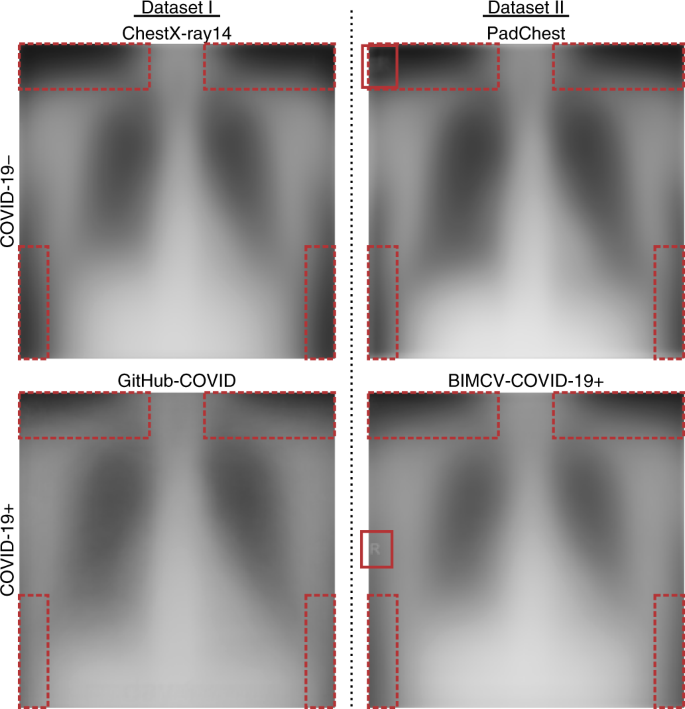
Average radiographs expose source signatures in laterality markers and image borders. Publisher figure from DeGrave, Janizek, and Lee (2021), Fig. 4.
Bias is not one thing
Representation and access
Who reaches care, enters the registry, has follow-up, and receives the intervention?
Measurement and labels
Whose physiology is measured accurately? What do codes and outcomes actually encode?
Evaluation
Which settings, eras, groups, and workflows are represented in validation?
Deployment and adoption
Who sees the tool, trusts it, is burdened by it, or can contest its consequences?
Fairness metrics can reveal some disparities. They cannot repair an ill-chosen purpose or an inequitable care pathway by themselves.
Fairness metrics: a mathematical lens
For a thresholded SSI-surveillance model, let:
- \(G\): an audit group;
- \(Y \in \{0,1\}\): the observed SSI outcome within a stated window;
- \(\hat p\): predicted risk;
- \(\hat Y_t=\mathbb{1}(\hat p\ge t)\): the positive decision at threshold \(t\).
| Flagged | Not flagged | |
|---|---|---|
| SSI observed | TP | FN |
| No SSI observed | FP | TN |
Four common comparisons use different denominators:
\[ \begin{aligned} \text{flag rate}_g &= P(\hat Y_t=1\mid G=g)\\ \text{TPR}_g &= P(\hat Y_t=1\mid Y=1,G=g)\\ \text{FPR}_g &= P(\hat Y_t=1\mid Y=0,G=g)\\ \text{PPV}_g &= P(Y=1\mid \hat Y_t=1,G=g). \end{aligned} \]
The denominator is the fairness question
These rates can tell different (and sometimes incompatible) stories. They also treat \(Y\) as the reference label, even when outcome ascertainment or follow-up may differ across groups. (Hardt, Price, and Srebro 2016; Chouldechova 2017)
Demographic parity: who is flagged?
Demographic parity asks for equal positive-decision rates:
\[ P(\hat Y_t=1\mid G=0)=P(\hat Y_t=1\mid G=1). \]
It may be relevant when
- the decision distributes access to a beneficial opportunity;
- equal access or allocation is the policy objective;
- observed differences may reflect an inequitable pathway into care.
It can mislead when
- the positive decision triggers a burden or treatment;
- outcome prevalence, follow-up, or clinical need differs;
- equal flag rates conceal unequal false-negative or false-positive rates.
Clinical interpretation
Equal rates of enhanced-surveillance flags do not, by themselves, establish equitable care. Ask what action follows, who can benefit, and who bears the burden. (Hardt, Price, and Srebro 2016)
Equalized odds: who is missed/burdened?
Equalized odds requires the positive-decision rate to be equal across groups within each observed outcome class: (Hardt, Price, and Srebro 2016)
\[ P(\hat Y_t=1\mid Y=y,G=0)=P(\hat Y_t=1\mid Y=y,G=1), \qquad y\in\{0,1\}. \]
Among cases with SSI
Equal TPR means the same proportion is flagged. Unequal TPR means one group experiences more missed opportunities for surveillance.
Among cases without SSI
Equal FPR means the same proportion is falsely flagged. Unequal FPR means one group experiences more unnecessary calls, visits, anxiety, or treatment.
Equal opportunity is the one-sided relaxation that equalizes TPR but does not require equal FPR. (Hardt, Price, and Srebro 2016)
Required assumption
The outcome definition, follow-up, and ascertainment must be comparable. Otherwise, error-rate parity may merely equalize performance against a differentially biased reference label.
Predictive parity and calibration: does the output mean the same thing?
Thresholded decision: predictive parity
\[ P(Y=1\mid \hat Y_t=1,G=0) =\\ P(Y=1\mid \hat Y_t=1,G=1). \]
Among people who are flagged, the same proportion experiences the observed outcome. This is equality of positive predictive value at the chosen threshold.
Risk score: calibration within groups
\[ P(Y=1\mid \hat p=p,G=g)\approx p. \]
Among people assigned a risk near \(p\), approximately a proportion \(p\) experiences the observed outcome—within each group.
Do not collapse these concepts
Equal PPV at one threshold is not full calibration. Groupwise calibration does not imply equal TPR, equal FPR, equal treatment, or equal clinical utility. (Chouldechova 2017; Kleinberg, Mullainathan, and Raghavan 2017)
Worked audit from patient-level records
Synthetic patient-level data (not AIRO). Each row represents one imagined patient (\(N=1000\)) with an observed SSI outcome and a model risk score.
Code
import numpy as np
import pandas as pd

rng = np.random.default_rng(5401)
threshold = 0.50

# Pedagogical design: same sample size, TPR, and FPR; different prevalence.
design = pd.DataFrame({
    "group": ["A", "B"],
    "n": [500, 500],
    "prevalence": [0.10, 0.04],
    "target_tpr": [0.80, 0.80],
    "target_fpr": [0.10, 0.10],
})


def make_group(spec):
    """Create patient-level outcomes and scores for one audit group."""
    n = int(spec["n"])
    n_positive = int(round(n * spec["prevalence"]))

    # Individual observed outcomes.
    y = np.r_[
        np.ones(n_positive, dtype=int),
        np.zeros(n - n_positive, dtype=int),
    ]
    rng.shuffle(y)

    # Select exactly the requested fraction of positives and negatives to flag.
    flagged = np.zeros(n, dtype=int)
    positive_idx = np.flatnonzero(y == 1)
    negative_idx = np.flatnonzero(y == 0)

    n_tp = int(round(spec["target_tpr"] * len(positive_idx)))
    n_fp = int(round(spec["target_fpr"] * len(negative_idx)))
    flagged[rng.choice(positive_idx, size=n_tp, replace=False)] = 1
    flagged[rng.choice(negative_idx, size=n_fp, replace=False)] = 1

    # Give each patient a score consistent with a thresholded model decision.
    risk_score = np.empty(n)
    risk_score[flagged == 1] = rng.uniform(
        threshold, 0.95, size=(flagged == 1).sum()
    )
    risk_score[flagged == 0] = rng.uniform(
        0.01, threshold, size=(flagged == 0).sum()
    )

    return pd.DataFrame({
        "group": spec["group"],
        "observed_ssi": y,
        "risk_score": risk_score,
    })


records = pd.concat(
    [make_group(spec) for _, spec in design.iterrows()],
    ignore_index=True,
)
records.insert(
    0,
    "patient_id",
    [f"SYN-{i:04d}" for i in range(1, len(records) + 1)],
)
records["flagged"] = (records["risk_score"] >= threshold).astype(int)
records = records.sample(frac=1, random_state=5401).reset_index(drop=True)


def audit_group(frame):
    """Compute confusion counts and threshold metrics from patient rows."""
    y = frame["observed_ssi"].to_numpy(dtype=bool)
    pred = frame["flagged"].to_numpy(dtype=bool)

    tp = int((y & pred).sum())
    fn = int((y & ~pred).sum())
    fp = int((~y & pred).sum())
    tn = int((~y & ~pred).sum())
    n = len(frame)

    return {
        "n": n,
        "events": int(y.sum()),
        "TP": tp,
        "FN": fn,
        "FP": fp,
        "TN": tn,
        "prevalence": y.mean(),
        "TPR": tp / (tp + fn),
        "FPR": fp / (fp + tn),
        "flag_rate": (tp + fp) / n,
        "PPV": tp / (tp + fp),
        "accuracy": (tp + tn) / n,
    }


metrics = pd.DataFrame({
    group: audit_group(frame)
    for group, frame in records.groupby("group", sort=True)
}).T

# Executable checks: fail the render if the constructed example drifts.
assert len(records) == 1000 and records["patient_id"].is_unique
np.testing.assert_allclose(metrics["TPR"], [0.80, 0.80])
np.testing.assert_allclose(metrics["FPR"], [0.10, 0.10])

pct = lambda value: f"{100 * value:.1f}%"
summary = pd.DataFrame(index=[
    "Patients",
    "Observed SSI cases",
    "TP / FN",
    "FP / TN",
    "TPR",
    "FPR",
    "Flag rate",
    "PPV",
    "Accuracy",
])

for group in metrics.index:
    m = metrics.loc[group]
    summary[f"Group {group}"] = [
        f"{int(m['n']):,}",
        f"{int(m['events'])} ({pct(m['prevalence'])})",
        f"{int(m['TP'])} / {int(m['FN'])}",
        f"{int(m['FP'])} / {int(m['TN'])}",
        pct(m["TPR"]),
        pct(m["FPR"]),
        pct(m["flag_rate"]),
        pct(m["PPV"]),
        pct(m["accuracy"]),
    ]

summary.index.name = "Quantity"
summary| Group A | Group B | |
|---|---|---|
| Quantity | ||
| Patients | 500 | 500 |
| Observed SSI cases | 50 (10.0%) | 20 (4.0%) |
| TP / FN | 40 / 10 | 16 / 4 |
| FP / TN | 45 / 405 | 48 / 432 |
| TPR | 80.0% | 80.0% |
| FPR | 10.0% | 10.0% |
| Flag rate | 17.0% | 12.8% |
| PPV | 47.1% | 25.0% |
| Accuracy | 89.0% | 89.6% |
Read, verify, then perturb
Equalized odds: TPR and FPR match. Demographic parity: flag rates differ. Predictive parity: PPV differs. Expand the code, inspect records, and then change Group B’s prevalence to 10%: the error rates stay fixed while PPV and the flag rate move.
Why fairness targets can conflict
Let the observed outcome prevalence in group \(g\) be
\[ \pi_g=P(Y=1\mid G=g). \]
At a fixed threshold,
\[ \operatorname{PPV}_g = \frac{\operatorname{TPR}_g\,\pi_g} {\operatorname{TPR}_g\,\pi_g+ \operatorname{FPR}_g(1-\pi_g)}. \]
If two groups have the same TPR and FPR but different prevalences, their PPVs generally differ. Conversely, forcing PPV to match may require unequal error rates, different thresholds, or changes to the underlying data and care process. (Chouldechova 2017; Kleinberg, Mullainathan, and Raghavan 2017)
An incompatibility, not a software defect
With unequal base rates and imperfect prediction, common fairness criteria cannot generally all be satisfied at once. Choosing what to equalize is therefore both a technical and a values decision. (Chouldechova 2017; Kleinberg, Mullainathan, and Raghavan 2017)
The fairness frame is part of an intervention
Access and allocation
Compare flag or selection rates when the decision distributes an opportunity or scarce resource.
Detection
Compare TPR when missed cases create unequal loss of access to an effective response.
Burden
Compare FPR—or both TPR and FPR—when false alarms create work, anxiety, visits, or treatment.
Meaning and trust
Compare PPV and groupwise calibration when clinicians or patients interpret the output as risk.
Before analysis, specify the groups, outcome window, action, threshold, primary fairness concern, acceptable trade-offs, and uncertainty analysis. Report denominators and event counts. (Hardt, Price, and Srebro 2016; Chouldechova 2017; Kleinberg, Mullainathan, and Raghavan 2017; Rajkomar et al. 2018)
A metric is only evidence
A disparity can identify where to investigate but does not, by itself, establish the cause or determine the remedy.
Privacy begins before deployment
Design-stage questions include:
- Is every variable necessary for the stated purpose?
- Who is authorized to access identifiable, linkable, or derived data?
- Can the study be completed inside a secure environment?
- What outputs may leave, and who reviews them?
- How will linkage keys, free text, logs, and model artifacts be handled?
- What obligations follow from community or Indigenous data governance?
Later
We will return to privacy as a technical and governance problem, including federated learning, cryptographic tools, differential privacy, and privacy–utility–fairness trade-offs.
How analysis is computed
A readiness bridge for clinical data science
This section reviews the technical grammar needed to read, run, critique, and extend a clinical ML study in practice.
We will refresh
- tables, arrays, masks, and vectorization;
- vectors, matrices, dot products, and shapes;
- probability, base rates, sampling, and uncertainty;
- plots, baselines, validation, and leakage.
We will keep asking
- What clinical process was active?
- Who is absent, mismeasured, or differently documented?
- What decision follows, and what happens when we are wrong?
- What evidence would make us change our minds?
Use this diagnostically
No one is expected to arrive equally fluent in every area. Notice where the reasoning becomes effortful. See 🔗 supporting resources.
Setup now = fewer headaches later
Because scientific results must be reproducible and dependable, record:
- the exact Python interpreter;
- installed package versions;
- the selected Jupyter kernel;
- operating-system and hardware details;
- data, cohort, and code versions.
Warning
A wrong kernel can produce a plausible answer with the wrong software stack. In clinical data science, that is a provenance error.
Recommended: Miniforge + conda-forge
- Install 🔗 Miniforge for your operating system.
- Open a new terminal (or the Miniforge prompt on 🙄 Windows).
- Verify the installation:
- If activation is unavailable, run
conda init, close the shell, and open it again.
Why Conda here?
Conda isolates Python and binary-heavy scientific packages. Our course examples use Python 3.11 for a stable, common baseline.
Clinical boundary
A software environment does not make health data safe. Use only approved storage, access, and disclosure processes for any non-synthetic data.
Create the DGIN 5401 environment
conda create -n dgin5401 -c conda-forge python=3.11 numpy pandas matplotlib scikit-learn jupyterlab ipykernel -y
conda activate dgin5401
Then verify the scientific stack:
- Install with Conda first.
- Use
python -m pip ...orpip install ...inside the activated environment only when a package is unavailable through your chosen Conda channel. - Avoid casually mixing channels: solver success is not the same as a coherent, reproducible environment.
Make Jupyter use the right Python
Register the activated environment as a Jupyter kernel:
In the notebook, select Python (DGIN 5401) and run:
The executable path should live inside the dgin5401 environment.
Conda gotcha: base is not the course
The base environment can become a dumping ground for unrelated projects. Keep course work in its own environment.
# Optional: stop base from activating in every new shell
conda config --set auto_activate_base false

# Start a course session
conda activate dgin5401

# The active environment has an asterisk
conda info --envs

# Both paths should point into dgin5401
python -c "import sys; print(sys.executable)"
python -m pip --version
Diagnostic habit
When an import fails or a notebook behaves strangely, check the active environment and kernel before reinstalling packages.
Freeze the environment before you report
Export the environment with the analysis:
A collaborator can reconstruct it with:
Also record the data version, cohort definition, code commit, random seed, model artifact, and evaluation configuration.
Reproducibility
environment.yml records software dependencies. We still need a data dictionary, analysis plan, model card, and a statement about the population.
Python mental model
- A variable name is a reference to an object.
- Objects have a type, a value, and often a shape.
- Many bugs are really mistaken assumptions about type, shape, or missingness.
Risk
"67", 67, and 67.0 may print similarly, but they do not behave identically.
Rows, columns, and shape
Code
shape: (3, 4)
first row: [ 67   1 121 119]
age column: [67 54 73]
Pause and discuss
Before running: is X[:, 0] one patient, one feature, or one prediction?
Boolean masks help filter
Code
[ True False  True False  True]
[67 73 81]
A mask has one truth value per element. Combining masks with &, |, and ~ is often clearer than a long loop.
Risk
Use parentheses around comparisons. In array code, and and or might not mean what you intend.
Axis compass
For a matrix X with shape (patients, features):
| Operation | Meaning |
|---|---|
X.mean(axis=0) |
one mean per feature |
X.mean(axis=1) |
one mean per patient |
X.sum() |
one total across everything |
X[:, j] |
feature j for all patients |
X[i, :] |
all features for patient i |
Pause and discuss
Which axis should be used to compute training-set means for feature standardization?
Broadcasting
Code
# Columns: pre-op haemoglobin (g/L), creatinine (µmol/L), bypass time (min)
X = np.array([[119., 82., 121.],
              [137., 71.,  88.],
              [108., 104., 176.]])

feature_means = X.mean(axis=0)   # one mean per clinical variable
patient_means = X.mean(axis=1)   # mixes incompatible units

print("feature-centred:\n", X - feature_means)
print("patient-centred:\n", X - patient_means[:, None])
feature-centred:
[[ -2.3333 -3.6667 -7.3333]
[ 15.6667 -14.6667 -40.3333]
[-13.3333 18.3333 47.6667]]
patient-centred:
[[ 11.6667 -25.3333 13.6667]
[ 38.3333 -27.6667 -10.6667]
[-21.3333 -25.3333 46.6667]]Both operations run. Only the first resembles a sensible preprocessing step. The second averages grams per litre, micromoles per litre, and minutes—as if those units shared a scale.
Clinical meaning
Syntactically valid array arithmetic can be scientifically or logically meaningless.
Pandas: inspect before modelling
import pandas as pd

df = pd.read_csv("cardiac_registry.csv")

print(df.shape)
print(df.dtypes)
print(df.head())
print(df.isna().mean().sort_values(ascending=False).head(15))
print(df["SSI_30d"].value_counts(dropna=False))
Data principle
Before fitting anything, verify identifiers, duplicated rows, units, impossible values, event prevalence, temporal coverage, and the provenance of every candidate predictor.
Missing values are not empty space
A blank may mean:
- “not measured because no one was concerned”;
- “not measured because the patient was unstable”;
- “not applicable”;
- “not documented”;
- “lost during extraction”;
- “removed or suppressed”; or
- a true negative event represented by absence.
Pause and discuss
For each important variable, write a sentence beginning: “This value is missing when…”
Fit preprocessing on training data only
from sklearn.impute import SimpleImputer
from sklearn.preprocessing import StandardScaler

imputer = SimpleImputer(strategy="median")
scaler = StandardScaler()

X_train_i = imputer.fit_transform(X_train)
X_train_s = scaler.fit_transform(X_train_i)

X_valid_s = scaler.transform(imputer.transform(X_valid))
X_test_s  = scaler.transform(imputer.transform(X_test))
Risk
If test-set values influence imputation, scaling, feature selection, or representation learning, the evaluation is contaminated.
Vectorization: same arithmetic, but clearer
# Loop
scores = []
for row in X:
    scores.append(sum(row[j] * w[j] for j in range(len(w))) + b)

# Vectorized
scores = X @ w + b
Vectorization can expose the mathematical structure and make shape errors easier to detect. It can also be a bit faster.
Reproducibility starts with the seed
Record:
- data version and extraction date;
- cohort query and label definition;
- train/validation/test membership;
- package and hardware versions;
- random seeds and search space;
- code commit and configuration;
- model artifact and calibration object.
Evidence
A result that cannot be reconstructed is difficult to audit, update, or trust. (Kapoor et al. 2024; Sendak et al. 2020)
What does “containerized” mean here?
A container image packages the application, runtime, dependencies, configuration, and startup command. A container is a running instance of that image. Docker and Podman are tools that build and run container images.
For this course, containerization supports reproducible local execution.
Vector = one measurement bundle
For one patient at one index time:
\[ \mathbf{x} = [\text{age},\;\text{diabetes},\;\text{bypass time},\;\text{haemoglobin}]^\top \]
A vector has:
- entries with meaning and units;
- a dimension;
- an orientation when multiplied;
- a coordinate system created by feature definitions and preprocessing.
Risk
A categorical code such as procedure type is not automatically a meaningful coordinate just because it is stored as an integer.
Matrix = many measurement bundles
\[ X = \begin{bmatrix} 67 & 1 & 121 & 119\\ 54 & 0 & 88 & 137\\ 73 & 1 & 176 & 108 \end{bmatrix} \]
Rows are patients or surgeries; columns are features.
The shape here is \(3\times4\): three examples, four features.
Pause and discuss
If w contains one weight per feature, what shape must w have for X @ w to work?
Dot product = an explainable score
\[ z = \mathbf{x}^{\top}\mathbf{w} + b = \sum_j x_j w_j + b \]
| Feature | Value \(x_j\) | Weight \(w_j\) | Contribution \(x_jw_j\) |
|---|---|---|---|
| age (standardized) | 0.7 | 0.30 | 0.21 |
| diabetes | 1 | 0.55 | 0.55 |
| bypass time | 1.1 | 0.44 | 0.48 |
| haemoglobin | -0.6 | -0.22 | 0.13 |
Model principle
For a linear model, contributions are exact decompositions of the score. They are not automatically causal explanations.
Matrix–vector multiplication = batch scoring
\[ \mathbf{z}=X\mathbf{w}+b \]
- each row of
Xis dotted with the samew; - the output has one score per row;
- the same model is applied consistently across the cohort;
- the score may then be transformed into a probability or class.
Bias or intercept = the starting score
\[ z = b + \sum_j x_jw_j \]
The intercept is the score when all encoded features are zero.
That interpretation depends on encoding:
- with raw age, zero may be clinically meaningless;
- after centring, zero may represent the training mean;
- with one-hot indicators, zero may represent a reference category.
Pause and discuss
Interpret the intercept only after you understand how every feature was encoded.
Categories become axes
Bad encoding:
This implies that “combined” is numerically farther from 🔗 CABG than valve is.
One-hot encoding:
Data principle
Encoding choices are assumptions about geometry.
Scale changes the geometry
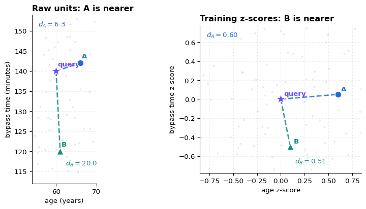
Illustrative patient vectors—not AIRO results. Euclidean distance treats one numerical unit on every feature axis as commensurate:
\[ d(\mathbf{x},\mathbf{z})=\lVert\mathbf{x}-\mathbf{z}\rVert_2. \]
Geometry is a modelling choice
The nearest neighbour changes even though the three patients do not. Scaling can be necessary, but it does not guarantee that numerical proximity is clinically meaningful.
Cosine similarity: angle, not length
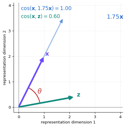
\[ \cos(\theta)= \frac{\mathbf{x}^{\top}\mathbf{z}} {\lVert\mathbf{x}\rVert\lVert\mathbf{z}\rVert} \]
- \(+1\): the same direction;
- \(0\): a right angle;
- \(-1\): opposite directions;
- multiplying a vector by a positive constant does not change its cosine similarity.
For text or representation embeddings, angle can be more useful than raw length.
Representation is not clinical equivalence
“Nearby in embedding space” does not mean clinically interchangeable, causally related, or safe to treat alike.
Z-score standardization
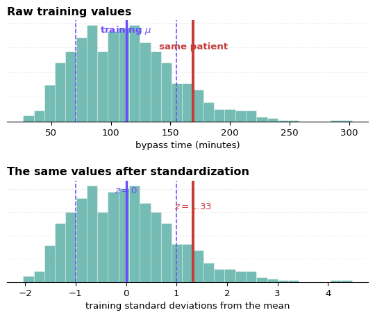
\[ z_{ij}=\frac{x_{ij}-\mu_j^{\text{train}}} {\sigma_j^{\text{train}}}. \]
- \(z=0\): the training mean;
- \(z=1\): one training standard deviation above;
- fit \(\mu_j\) and \(\sigma_j\) on the training set only;
- apply those same values to validation, test, and future data.
What is preserved
Ordering and distributional shape remain the same. The transformation changes location and scale—not the underlying observations.
Standardization does not make data Gaussian
It does not remove skew, outliers, missingness, or site shift. Preserve the fitted transformer with the model and monitor future z-scores against the training distribution.
How results become evidence
Function, loss, and parameter
A model \(f_\theta\) maps inputs to predictions. A loss measures how undesirable those predictions are on training examples.
\[ \hat y_i=f_\theta(\mathbf{x}_i), \qquad \mathcal{L}(\theta)=\frac{1}{n}\sum_i \ell(y_i,\hat y_i) \]
- \(\theta\): parameters learned from data;
- \(\ell\): per-example penalty;
- \(\mathcal{L}\): aggregate objective;
- metric: evaluation summary, not necessarily the training loss.
Derivative = local change
\[ f'(x)=\lim_{h\to0}\frac{f(x+h)-f(x)}{h} \]
A derivative answers:
If we change this input or parameter slightly, how does the output change locally?
It does not describe the whole function, guarantee linearity, or tell us whether changing a clinical variable would cause a different outcome.
Partial derivatives and gradients
For a loss depending on many parameters:
\[ \nabla_\theta \mathcal{L}= \begin{bmatrix} \frac{\partial \mathcal{L}}{\partial \theta_1}\\ \vdots\\ \frac{\partial \mathcal{L}}{\partial \theta_p} \end{bmatrix} \]
The gradient points in the direction of steepest local increase. To reduce the loss, move in the opposite direction.
Gradient descent: follow the loss downhill
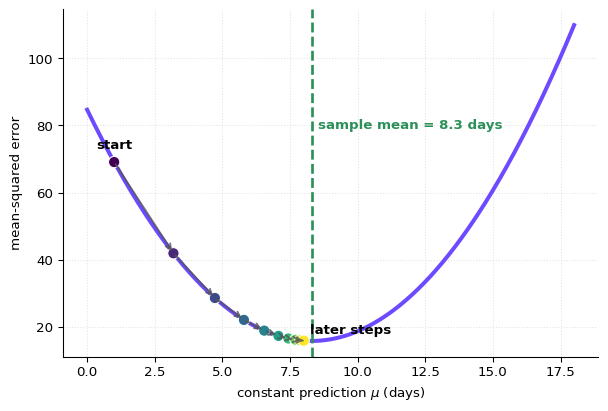
Consider the constant predictor:
\[ \mathcal{L}(\mu)=\frac{1}{n}\sum_i(y_i-\mu)^2 \]
\[ \mu_{t+1}=\mu_t- \eta\frac{d\mathcal{L}}{d\mu}. \]
- the gradient is the local slope;
- \(-\nabla\mathcal{L}\) points downhill;
- \(\eta\) controls the step size;
- under mean-squared error, the optimum constant is the sample mean.
The chain rule is dependency accounting
If \(y=f(u)\) and \(u=g(x)\), then
\[ \frac{dy}{dx}=\frac{dy}{du}\frac{du}{dx}. \]
Neural-network backpropagation repeatedly applies this rule through a graph of operations.
Sigmoid: score to bounded output
\[ \sigma(z)=\frac{1}{1+e^{-z}} \]
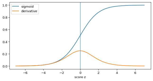
A sigmoid output is not automatically a well-calibrated probability; calibration is an empirical property of model predictions in a population.
Probability grammar: regions in a patient population
Let \(A=\) observed SSI and \(B=\) model alert. A probability is the share of the reference population that falls in a region.
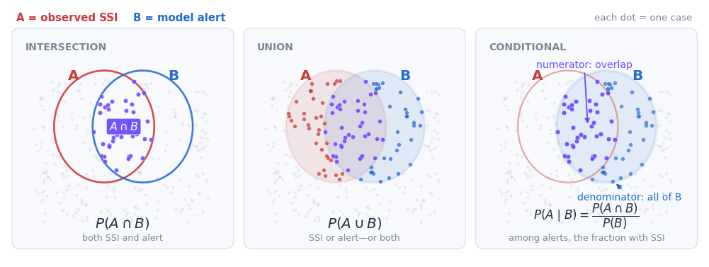
Read the conditional in words
\(P(A\mid B)\) asks: among the cases in \(B\), what fraction are also in \(A\)?
Bayes with natural frequencies
Suppose 1,000 surgeries have:
- 5% SSI prevalence → 50 infections;
- 80% sensitivity → 40 true alerts;
- 90% specificity → 95 false alerts among 950 non-infections.
Then:
\[ P(\text{SSI}\mid\text{alert})=\frac{40}{40+95}\approx 30\%. \]
Evidence
Even a useful test can produce many false alerts when the outcome is uncommon. Always remember your priors!
Base-rate visual
Code
n = 1000
prevalence = 0.05
sensitivity = 0.80
specificity = 0.90

y = np.zeros(n, dtype=int)
y[:int(n*prevalence)] = 1
pred = np.zeros(n, dtype=int)
pred[:int(n*prevalence*sensitivity)] = 1
start_neg = int(n*prevalence)
pred[start_neg:start_neg+int((n-start_neg)*(1-specificity))] = 1

# shuffle only for display
rng = np.random.default_rng(5401)
idx = rng.permutation(n)
y, pred = y[idx], pred[idx]
color_code = np.where((y==1)&(pred==1), 3,
              np.where((y==0)&(pred==1), 2,
              np.where((y==1)&(pred==0), 1, 0))).reshape(20,50)
from matplotlib.colors import ListedColormap, BoundaryNorm
from matplotlib.patches import Patch

# colour_code:
# 0 = true negative, 1 = false negative,
# 2 = false positive, 3 = true positive
TN_COLOUR = "#d9dee7"

tile_colours = [
    TN_COLOUR,  # true negative: no SSI, no alert
    RISK,       # false negative: SSI, no alert
    DAL_GOLD,   # false positive: no SSI, alert
    CLINICAL,   # true positive: SSI, alert
]

cmap = ListedColormap(tile_colours)
norm = BoundaryNorm(np.arange(-0.5, 4.5, 1), cmap.N)

fig, ax = plt.subplots(figsize=(10, 4.5))

ax.imshow(
    color_code,
    cmap=cmap,
    norm=norm,
    aspect="auto",
    interpolation="nearest",
)

ax.set_xticks([])
ax.set_yticks([])
ax.set_title(
    "1,000 surgeries: true and false alerts under a 5% base rate"
)

# Recalculate the legend counts from the displayed patient tiles.
tn, fn, fp, tp = np.bincount(
    color_code.ravel(),
    minlength=4,
)

legend_handles = [
    Patch(
        facecolor=CLINICAL,
        edgecolor="white",
        label=f"True positive: SSI + alert (n={tp})",
    ),
    Patch(
        facecolor=DAL_GOLD,
        edgecolor="white",
        label=f"False positive: no SSI + alert (n={fp})",
    ),
    Patch(
        facecolor=RISK,
        edgecolor="white",
        label=f"False negative: SSI + no alert (n={fn})",
    ),
    Patch(
        facecolor=TN_COLOUR,
        edgecolor="#9aa4b2",
        label=f"True negative: no SSI + no alert (n={tn})",
    ),
]

ax.legend(
    handles=legend_handles,
    loc="upper center",
    bbox_to_anchor=(0.5, -0.05),
    ncol=2,
    frameon=False,
    fontsize=10,
    handlelength=1.5,
    columnspacing=2.2,
)

fig.subplots_adjust(bottom=0.25)
plt.show()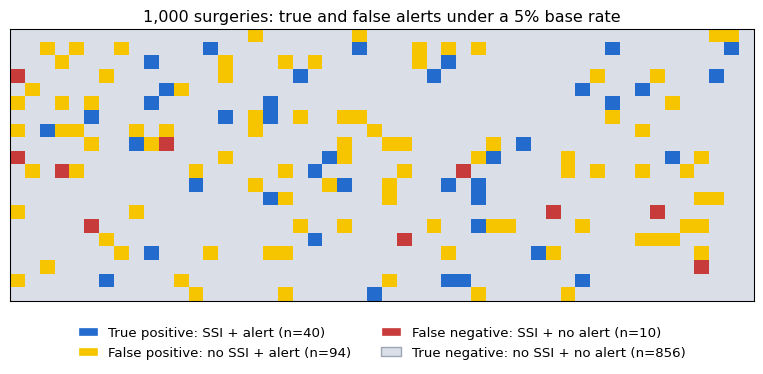
Random variables and expected value
For binary SSI outcome \(Y\in\{0,1\}\):
\[ E[Y]=P(Y=1), \qquad Var(Y)=p(1-p). \]
For a predicted risk \(\hat p\), the expected number of infections in a group is approximately \(\sum_i \hat p_i\) only when predictions are calibrated for that group.
Same mean, different operational risk
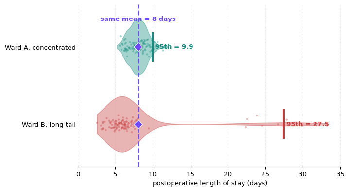
Don’t jump to conclusions
A long tail may reflect patients, different care pathways, complications, transfer practices, missingness, or data error. Investigate before interpreting or deleting outliers.
Both wards average 8 days, but Ward B has a much longer tail.
That difference can change:
- bed occupancy and staffing pressure;
- the number of unusually complex cases;
- the usefulness of a mean-based baseline;
- the consequences of prediction error.
Report distributions, quantiles, and tail probabilities—not only averages.
Bootstrap intuition: measuring uncertainty
Code
rng = np.random.default_rng(5401)
los_days = rng.gamma(shape=2.2, scale=3.0, size=80)
boot_means = np.array([
    rng.choice(los_days, size=len(los_days), replace=True).mean()
    for _ in range(2000)
])
lo, hi = np.quantile(boot_means, [0.025, 0.975])
print({
    "sample_mean_days": round(los_days.mean(), 2),
    "bootstrap_95%": (round(lo, 2), round(hi, 2)),
})
fig, ax = plt.subplots(figsize=(7, 3.4))
ax.hist(boot_means, bins=35)
ax.axvline(lo, linestyle="--")
ax.axvline(hi, linestyle="--")
ax.set_xlabel("bootstrap mean postoperative length of stay (days)")
plt.show()
{'sample_mean_days': np.float64(5.97), 'bootstrap_95%': (np.float64(5.19), np.float64(6.75))}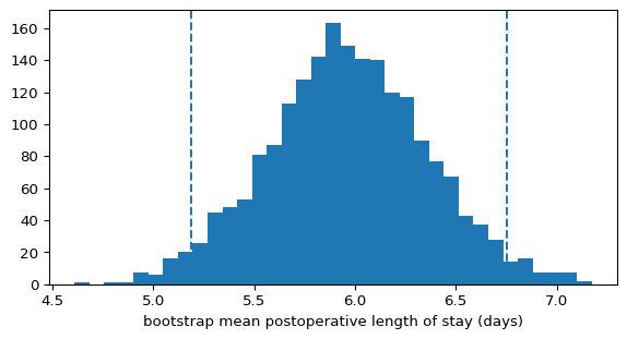
The interval reflects resampling uncertainty under assumptions about how the observed surgeries represent the target population. It does not capture unmeasured site shift, label error, or a changed care pathway.
Baseline first
Before a sophisticated model, compare against:
- prevalence-only prediction;
- simple clinical score or rule;
- regularized logistic regression;
- current workflow or clinician judgement;
- previous validated model;
- “treat all” and “treat none” policies where relevant.
Evidence
A complex model that barely beats a strong baseline may not justify added maintenance, opacity, latency, or governance burden.
Clean workflow versus leaky workflow
Code
flowchart LR
  A[Raw cohort] --> B[Split by patient/time/site]
  B --> C[Fit preprocessing on train]
  C --> D[Fit model on train]
  D --> E[Tune on validation]
  E --> F[One final test evaluation]
Code
flowchart LR
  X[All data] --> Y[Impute/scale/select on everything]
  Y --> Z[Random row split]
  Z --> Q[Repeatedly inspect test score]
  Q --> R[Optimistic claim]
Risk
Leakage is information crossing a boundary that the claimed deployment would not allow. (Kapoor and Narayanan 2023; Varoquaux and Cheplygina 2022)
Intervention can reverse an association
target mistake
The pneumonia risk model of Caruana et al. (2015) appeared to learn that asthma lowered pneumonia mortality risk.

Cropped from Caruana et al. (2015), Fig. 1.
What the model had learned was a channel effect: patients with asthma and pneumonia were more likely to be treated vigorously, including ICU admission.
So the model captured part of the care pathway, not just the disease process.
Note
To a large extent, realizing this is an early victory of ‘explainable AI’.
Prediction (and correlation) is not causation
A model can predict SSI using features that are:
- causes of infection;
- consequences of early infection;
- proxies for clinical concern;
- markers of hospital, surgeon, or time period;
- artifacts of documentation;
- correlated with access to follow-up.
Good prediction tends to minimize a loss, on training data.
Causal inference asks “what would change under an intervention?”
Research models and widely deployed proprietary models have shown why external validation matters. (Futoma, Hariharan, and Heller 2017; Wong et al. 2021)
Legacy case: readmission
Readmission risk can support follow-up planning, but it is influenced by:
- disease severity and recovery;
- discharge readiness and education;
- access to primary and specialty care;
- social support, transportation, and medication access;
- coding and cross-hospital visibility;
- competing events and planned readmissions.
Pause and discuss
What action is available for a high-risk patient, and who has capacity to provide it?
Foundations evidence statement
In
[population and setting], using information available by[index time], model[name/version]estimated[outcome/horizon]. On[evaluation design], it achieved[discrimination, calibration, and uncertainty]. Performance was[subgroup/temporal summary]. At threshold[t], the expected workload and errors were[counts/rates]. These results support[narrow claim], but do not establish[causal or deployment claim].
Pause and discuss
A strong evidence statement is modest, specific, reproducible, and tied to a decision.
Foundations self-check
You are ready to continue when you can:
- read array shapes and explain an axis operation;
- interpret a dot product as a score;
- explain a gradient update conceptually;
- distinguish sensitivity from precision;
- reason with a base rate using counts;
- identify preprocessing leakage;
- state uncertainty and limits around a result;
- ask what decision follows from a prediction.
Exercise · audit a synthetic extraction
A table contains one row per surgery_id, but you discover:
| Finding | Example |
|---|---|
| duplicated patients | two surgeries from the same person split across train and test |
| mixed units | creatinine values around 1.1 and 98 in one column |
| late information | “discharge antibiotics” used for an ICU-transfer model |
| informative missingness | lactate measured mainly when clinicians are worried |
| join expansion | one surgery becomes eight rows after joining notes |
| era marker | a form field appears only after a registry redesign |
For each finding, how do we: detect, repair, document, and estimate risk.
Which problems are coding errors, which are study-design errors, and which are properties of care?
References
Agniel, Denis, Isaac S. Kohane, and Griffin M. Weber. 2018. “Biases in Electronic Health Record Data Due to Processes Within the Healthcare System: Retrospective Observational Study.” BMJ 361: k1479. https://doi.org/10.1136/bmj.k1479.
Alaa, Ahmed M., Boris van Breugel, Evgeny S. Saveliev, and Mihaela van der Schaar. 2022. “How Faithful Is Your Synthetic Data? Sample-Level Metrics for Evaluating and Auditing Generative Models.” In Proceedings of the 39th International Conference on Machine Learning, 162:290–306. Proceedings of Machine Learning Research. PMLR.
Alderman, Jessica E., John Palmer, Edward Laws, Melissa D. McCradden, et al. 2025. “Tackling Algorithmic Bias and Promoting Transparency in Health Datasets: The STANDING Together Consensus Recommendations.” The Lancet Digital Health 7 (1): e64–88. https://doi.org/10.1016/S2589-7500(24)00224-3.
Bhanot, Karan, Miao Qi, John S. Erickson, Isabelle Guyon, and Kristin P. Bennett. 2021. “The Problem of Fairness in Synthetic Healthcare Data.” Entropy 23 (9): 1165. https://doi.org/10.3390/e23091165.
Bland, J. Martin, and Douglas G. Altman. 1986. “Statistical Methods for Assessing Agreement Between Two Methods of Clinical Measurement.” The Lancet 1 (8476): 307–10. https://doi.org/10.1016/S0140-6736(86)90837-8.
Bucher, Brian T., Jianlin Shi, Jeffrey P. Ferraro, David E. Skarda, Matthew H. Samore, John F. Hurdle, Adi V. Gundlapalli, Wendy W. Chapman, and Samuel R. G. Finlayson. 2020. “Portable Automated Surveillance of Surgical Site Infections Using Natural Language Processing: Development and Validation.” Annals of Surgery 272 (4): 629–36. https://doi.org/10.1097/SLA.0000000000004133.
Caruana, Rich, Yin Lou, Johannes Gehrke, Paul Koch, Marc Sturm, and Noémie Elhadad. 2015. “Intelligible Models for HealthCare: Predicting Pneumonia Risk and Hospital 30-Day Readmission.” In Proceedings of the 21th ACM SIGKDD International Conference on Knowledge Discovery and Data Mining, 1721–30. https://doi.org/10.1145/2783258.2788613.
Chouldechova, Alexandra. 2017. “Fair Prediction with Disparate Impact: A Study of Bias in Recidivism Prediction Instruments.” Big Data 5 (2): 153–63. https://doi.org/10.1089/big.2016.0047.
Cicchetti, Domenic V., and Alvan R. Feinstein. 1990. “High Agreement but Low Kappa: II. Resolving the Paradoxes.” Journal of Clinical Epidemiology 43 (6): 551–58. https://doi.org/10.1016/0895-4356(90)90159-M.
Cohen, Jacob. 1960. “A Coefficient of Agreement for Nominal Scales.” Educational and Psychological Measurement 20 (1): 37–46. https://doi.org/10.1177/001316446002000104.
———. 1968. “Weighted Kappa: Nominal Scale Agreement with Provision for Scaled Disagreement or Partial Credit.” Psychological Bulletin 70 (4): 213–20. https://doi.org/10.1037/h0026256.
Collins, Gary S., Paul Dhiman, Jia Ma, Michael Schlussel, Luke Archer, Ben Van Calster, et al. 2024. “Evaluation of Clinical Prediction Models (Part 1): From Development to External Validation.” BMJ 384: e074819. https://doi.org/10.1136/bmj-2023-074819.
Davis, Sharon E., Michael E. Matheny, Suresh Balu, and Mark P. Sendak. 2024. “A Framework for Understanding Label Leakage in Machine Learning for Health Care.” Journal of the American Medical Informatics Association 31 (1): 274–80. https://doi.org/10.1093/jamia/ocad178.
DeGrave, Alex J., Joseph D. Janizek, and Su-In Lee. 2021. “AI for Radiographic COVID-19 Detection Selects Shortcuts over Signal.” Nature Machine Intelligence 3 (7): 610–19. https://doi.org/10.1038/s42256-021-00338-7.
El Emam, Khaled, Lucy Mosquera, Xi Fang, and Alaa El-Hussuna. 2024. “An Evaluation of the Replicability of Analyses Using Synthetic Health Data.” Scientific Reports 14: 6978. https://doi.org/10.1038/s41598-024-57207-7.
Feinstein, Alvan R., and Domenic V. Cicchetti. 1990. “High Agreement but Low Kappa: I. The Problems of Two Paradoxes.” Journal of Clinical Epidemiology 43 (6): 543–49. https://doi.org/10.1016/0895-4356(90)90158-L.
Fleiss, Joseph L. 1971. “Measuring Nominal Scale Agreement Among Many Raters.” Psychological Bulletin 76 (5): 378–82. https://doi.org/10.1037/h0031619.
Ford, Elizabeth, John A. Carroll, Helen E. Smith, Donia Scott, and Jackie A. Cassell. 2016. “Extracting Information from the Text of Electronic Medical Records to Improve Case Detection: A Systematic Review.” Journal of the American Medical Informatics Association 23 (5): 1007–15. https://doi.org/10.1093/jamia/ocv180.
Futoma, Joseph, Sanjay Hariharan, and Katherine Heller. 2017. “Learning to Detect Sepsis with a Multitask Gaussian Process RNN Classifier.” In Proceedings of Machine Learning for Healthcare, 68:117–35. Proceedings of Machine Learning Research. https://proceedings.mlr.press/v68/futoma17a.html.
Giomi, Matteo, Franziska Boenisch, Christoph Wehmeyer, and Borbála Tasnádi. 2023. “A Unified Framework for Quantifying Privacy Risk in Synthetic Data.” Proceedings on Privacy Enhancing Technologies 2023 (2): 312–28. https://doi.org/10.56553/popets-2023-0055.
Goldberger, Ary L., Luis A. N. Amaral, Leon Glass, Jeffrey M. Hausdorff, Plamen Ch. Ivanov, Roger G. Mark, Joseph E. Mietus, George B. Moody, Chung-Kang Peng, and H. Eugene Stanley. 2000. “PhysioBank, PhysioToolkit, and PhysioNet: Components of a New Research Resource for Complex Physiologic Signals.” Circulation 101 (23): e215–20. https://doi.org/10.1161/01.CIR.101.23.e215.
Groenwold, Rolf H. H. 2020. “Informative Missingness in Electronic Health Record Systems: The Curse of Knowing.” Diagnostic and Prognostic Research 4: 8. https://doi.org/10.1186/s41512-020-00077-0.
Gwet, Kilem Li. 2008. “Computing Inter-Rater Reliability and Its Variance in the Presence of High Agreement.” British Journal of Mathematical and Statistical Psychology 61 (1): 29–48. https://doi.org/10.1348/000711006X126600.
Hardt, Moritz, Eric Price, and Nathan Srebro. 2016. “Equality of Opportunity in Supervised Learning.” In Advances in Neural Information Processing Systems, 29:3315–23. Curran Associates, Inc. https://arxiv.org/abs/1610.02413.
Harkema, Henk, John N. Dowling, Tyler Thornblade, and Wendy W. Chapman. 2009. “ConText: An Algorithm for Determining Negation, Experiencer, and Temporal Status from Clinical Reports.” Journal of Biomedical Informatics 42 (5): 839–51. https://doi.org/10.1016/j.jbi.2009.05.002.
Hayes, Andrew F., and Klaus Krippendorff. 2007. “Answering the Call for a Standard Reliability Measure for Coding Data.” Communication Methods and Measures 1 (1): 77–89. https://doi.org/10.1080/19312450709336664.
Houssiau, Florimond, James Jordon, Samuel N. Cohen, Owen Daniel, Andrew Elliott, James Geddes, Callum Mole, Camila Rangel-Smith, and Lukasz Szpruch. 2022. “TAPAS: A Toolbox for Adversarial Privacy Auditing of Synthetic Data.” arXiv Preprint arXiv:2211.06550. https://doi.org/10.48550/arXiv.2211.06550.
Johnson, Alistair E. W., Lucas Bulgarelli, Lu Shen, Alvin Gayles, Ayad Shammout, Steven Horng, Tom J. Pollard, et al. 2023. “MIMIC-IV, a Freely Accessible Electronic Health Record Dataset.” Scientific Data 10: 1. https://doi.org/10.1038/s41597-022-01899-x.
Kaabachi, Bayrem, Jérémie Despraz, Thierry Meurers, Karen Otte, Mehmed Halilovic, Bogdan Kulynych, Fabian Prasser, et al. 2025. “A Scoping Review of Privacy and Utility Metrics in Medical Synthetic Data.” Npj Digital Medicine 8: 60. https://doi.org/10.1038/s41746-024-01359-3.
Kapoor, Sayash, Emily M. Cantrell, Kenny Peng, Tuan H. Pham, Christopher A. Bail, Odd Erik Gundersen, et al. 2024. “REFORMS: Consensus-Based Recommendations for Machine-Learning-Based Science.” Science Advances 10 (18): eadk3452. https://doi.org/10.1126/sciadv.adk3452.
Kapoor, Sayash, and Arvind Narayanan. 2023. “Leakage and the Reproducibility Crisis in Machine-Learning-Based Science.” Patterns 4 (9): 100804. https://doi.org/10.1016/j.patter.2023.100804.
Kleinberg, Jon, Sendhil Mullainathan, and Manish Raghavan. 2017. “Inherent Trade-Offs in the Fair Determination of Risk Scores.” In 8th Innovations in Theoretical Computer Science Conference (ITCS 2017), 67:43:1–23. Leibniz International Proceedings in Informatics (LIPIcs). Schloss Dagstuhl–Leibniz-Zentrum für Informatik. https://doi.org/10.4230/LIPIcs.ITCS.2017.43.
Kottner, Jan, Laurent Audigé, Stig Brorson, Allan Donner, Byron J. Gajewski, Asbjørn Hróbjartsson, Chris Roberts, Mohamed Shoukri, and David L. Streiner. 2011. “Guidelines for Reporting Reliability and Agreement Studies (GRRAS) Were Proposed.” Journal of Clinical Epidemiology 64 (1): 96–106. https://doi.org/10.1016/j.jclinepi.2010.03.002.
Nestor, Bret, Matthew B. A. McDermott, Willie Boag, Gabriela Berner, Tristan Naumann, Michael C. Hughes, Anna Goldenberg, and Marzyeh Ghassemi. 2019. “Feature Robustness in Non-Stationary Health Records: Caveats to Deployable Model Performance in Common Clinical Machine Learning Tasks.” In Proceedings of the 4th Machine Learning for Healthcare Conference, 106:381–405. Proceedings of Machine Learning Research. PMLR. https://proceedings.mlr.press/v106/nestor19a.html.
Obermeyer, Ziad, Brian Powers, Christine Vogeli, and Sendhil Mullainathan. 2019. “Dissecting Racial Bias in an Algorithm Used to Manage the Health of Populations.” Science 366 (6464): 447–53. https://doi.org/10.1126/science.aax2342.
Pilgram, Lisa, Fida Kamal Dankar, Jörg Drechsler, Mark Elliot, Josep Domingo-Ferrer, Paul Francis, Murat Kantarcioglu, et al. 2025. “A Consensus Privacy Metrics Framework for Synthetic Data.” Patterns 6 (10): 101320. https://doi.org/10.1016/j.patter.2025.101320.
Pilgram, Lisa, Haksoo Ko, Adeline Tung, and Khaled El Emam. 2025. “Protecting Patient Privacy in Tabular Synthetic Health Data: A Regulatory Perspective.” Npj Digital Medicine 8: 732. https://doi.org/10.1038/s41746-025-02112-0.
Rajkomar, Alvin, Michaela Hardt, Michael D. Howell, Greg Corrado, and Marshall H. Chin. 2018. “Ensuring Fairness in Machine Learning to Advance Health Equity.” Annals of Internal Medicine 169 (12): 866–72. https://doi.org/10.7326/M18-1990.
Rule, Adam, Steven Bedrick, Michael F. Chiang, and Michelle R. Hribar. 2021. “Length and Redundancy of Outpatient Progress Notes Across a Decade at an Academic Medical Center.” JAMA Network Open 4 (7): e2115334. https://doi.org/10.1001/jamanetworkopen.2021.15334.
Schwabe, Daniel, Michael Becker, Julia Seyferth, et al. 2024. “The METRIC-Framework for Assessing Data Quality for Trustworthy AI in Medicine: A Systematic Review.” Npj Digital Medicine 7. https://doi.org/10.1038/s41746-024-01196-4.
Sendak, Mark P., John D’Arcy, Sonoo Kashyap, Michael Gao, Mike Nichols, Kristin Corey, William Ratliff, and Suresh Balu. 2020. “A Path for Translation of Machine Learning Products into Healthcare Delivery.” Npj Digital Medicine 3: 132. https://doi.org/10.1038/s41746-020-00327-1.
Shrout, Patrick E., and Joseph L. Fleiss. 1979. “Intraclass Correlations: Uses in Assessing Rater Reliability.” Psychological Bulletin 86 (2): 420–28. https://doi.org/10.1037/0033-2909.86.2.420.
Sjoding, Michael W., Robert P. Dickson, Theodore J. Iwashyna, Steven E. Gay, and Thomas S. Valley. 2020. “Racial Bias in Pulse Oximetry Measurement.” New England Journal of Medicine 383: 2477–78. https://doi.org/10.1056/NEJMc2029240.
Suresh, Harini, and John V. Guttag. 2021. “A Framework for Understanding Sources of Harm Throughout the Machine Learning Life Cycle.” In Proceedings of the 1st ACM Conference on Equity and Access in Algorithms, Mechanisms, and Optimization. https://doi.org/10.1145/3465416.3483305.
Varoquaux, Gaël, and Veronika Cheplygina. 2022. “Machine Learning for Medical Imaging: Methodological Failures and Recommendations for the Future.” Npj Digital Medicine 5: 48. https://doi.org/10.1038/s41746-022-00592-y.
Wong, Andrew, Erkin Otles, John P. Donnelly, Anne Krumm, James McCullough, Olivia DeTroyer-Cooley, et al. 2021. “External Validation of a Widely Implemented Proprietary Sepsis Prediction Model in Hospitalized Patients.” JAMA Internal Medicine 181 (8): 1065–70. https://doi.org/10.1001/jamainternmed.2021.2626.
Yan, Chao, Yao Yan, Zhiyu Wan, Ziqi Zhang, Larsson Omberg, Justin Guinney, Sean D. Mooney, and Bradley A. Malin. 2022. “A Multifaceted Benchmarking of Synthetic Electronic Health Record Generation Models.” Nature Communications 13: 7609. https://doi.org/10.1038/s41467-022-35295-1.

DGIN 5401 · Operationalized ML in Healthcare