Can we get more useful supervision without hand-labeling everything?
Learning outcomes
By the end of this module, you should be able to:
explain why self-supervised and semi-supervised learning become attractive when labels are scarce but raw data is abundant;
distinguish supervised, semi-supervised, and self-supervised objectives in terms of what supervision signal is available;
analyze the cluster / low-density assumptions that often justify semi-supervised methods;
implement a simple pseudo-labeling or consistency-regularization baseline and evaluate it critically;
justify when a self-supervised pretext task is likely to help a downstream task, and when it may fail.
The central picture
Code
flowchart LR
    A[Raw data<br/>lots of examples] --> B{Do we have labels?}
    B -->|many labels| C[Supervised learning]
    B -->|few labels +<br> many unlabeled examples| D[Semi-supervised learning]
    B -->|no task labels but <br>structure in data| E[Self-supervised learning]
    E --> F[Learn representations]
    F --> G[Fine-tune / linear probe / <br>transfer]
    D --> H[Joint supervised + unlabeled-data objective]
flowchart LR
    A[Raw data<br/>lots of examples] --> B{Do we have labels?}
    B -->|many labels| C[Supervised learning]
    B -->|few labels +<br> many unlabeled examples| D[Semi-supervised learning]
    B -->|no task labels but <br>structure in data| E[Self-supervised learning]
    E --> F[Learn representations]
    F --> G[Fine-tune / linear probe / <br>transfer]
    D --> H[Joint supervised + unlabeled-data objective]
The difference is not that one is “more advanced.”
The difference is where the training signal comes from.
Conceptual scaffold
A quick decision heuristic
Code
flowchart TD
    A[Need a model for a <br>downstream task] --> B{How many trusted labels<br> do you have?}
    B -->|enough| C[Start supervised]
    B -->|few| D{Do you also have lots<br>of unlabeled data?}
    D -->|no| E[Collect labels or simplify task]
    D -->|yes| F{Can you define a useful<br>pretext task or augmentation?}
    F -->|yes| G[Try self-supervised pretraining]
    F -->|also yes for same task| H[Try semi-supervised training]
    G --> I[Fine-tune / linear probe]
    H --> I
flowchart TD
    A[Need a model for a <br>downstream task] --> B{How many trusted labels<br> do you have?}
    B -->|enough| C[Start supervised]
    B -->|few| D{Do you also have lots<br>of unlabeled data?}
    D -->|no| E[Collect labels or simplify task]
    D -->|yes| F{Can you define a useful<br>pretext task or augmentation?}
    F -->|yes| G[Try self-supervised pretraining]
    F -->|also yes for same task| H[Try semi-supervised training]
    G --> I[Fine-tune / linear probe]
    H --> I
Use this as a rule of thumb:
semi-supervised when unlabeled data should help the same task directly;
self-supervised when unlabeled data can first help learn a good representation.
Precise definitions
Let
\(\mathcal{D}_L = \{(x_i, y_i)\}_{i=1}^{n_L}\) be labeled data,
\(\mathcal{D}_U = \{x_j\}_{j=1}^{n_U}\) be unlabeled data.
Supervised learning uses only \(\mathcal{D}_L\) to learn the task \(x \mapsto y\).
Semi-supervised learning uses both \(\mathcal{D}_L\) and \(\mathcal{D}_U\)for the same downstream task.
Self-supervised learning creates a training signal from the data itself, for example by:
masking part of the input and predicting it;
reconstructing a corrupted input;
bringing two views of the same example closer in representation space.
A helpful distinction:
Semi-supervised asks: How can unlabeled data help the supervised task directly?
Self-supervised asks: How can I learn useful representations before I even have many labels?
Three common patterns
Code
flowchart TD
    A[Input x] --> B[Corrupt / mask / augment x]
    B --> C[Predict missing part<br/>or match two views]
    C --> D[Representation z]

    E[Labeled subset] --> F[Task loss]
    D --> F
    G[Unlabeled subset] --> H[Consistency or<br>pseudo-label signal]
    H --> F
flowchart TD
    A[Input x] --> B[Corrupt / mask / augment x]
    B --> C[Predict missing part<br/>or match two views]
    C --> D[Representation z]

    E[Labeled subset] --> F[Task loss]
    D --> F
    G[Unlabeled subset] --> H[Consistency or<br>pseudo-label signal]
    H --> F
Read this as:
self-supervised: create a pretext task to learn \(z\);
semi-supervised: combine task loss with an unlabeled-data loss;
sometimes we do both in sequence.
The key assumptions
These methods help only when the unlabeled data tells us something useful about task structure.
Common assumptions:
Cluster assumption
points in the same high-density region should usually share a label.
Low-density separation
good decision boundaries should avoid dense regions of data.
Augmentation / invariance assumption
label-preserving transformations should not change the prediction much.
Transfer assumption
the pretext task must force the model to learn features that are useful later.
If these assumptions fail, unlabeled data can actively mislead the model.
❌ Anti-example: when the idea is misused
Suppose we build pseudo-labels for a medical-image classifier using high confidence on an unlabeled hospital dataset.
That can go wrong if:
the unlabeled pool comes from a different scanner or population;
the model is confidently wrong on minority subgroups;
we treat all transformations as label-preserving when some are not;
we add thousands of pseudo-labels and drown out the few trusted labels.
This is a classic anti-example:
“More data” is not the same thing as “more correct supervision.”
Unlabeled data is only helpful when its structure aligns with the target task and data-generating process.
pseudo-labeling
use the model’s own high-confidence predictions as temporary labels;
consistency regularization
require similar predictions for two perturbations \(t_1(x), t_2(x)\).
The tuning parameter \(\lambda\) matters:
too small and unlabeled data does little; too large and noisy pseudo-supervision can dominate.
Self-supervised objectives
Three common examples:
1. Reconstruction / denoising(Vincent et al. 2010)\[
\mathcal{L}_{\text{denoise}}(\theta)
=
\sum_x \| g_\theta(\tilde{x}) - x \|^2
\] where \(\tilde{x}\) is a corrupted version of \(x\).
then placing a decision boundary inside that dense region creates lots of local disagreements and increases loss.
So, under the cluster assumption, minimizing consistency loss tends to encourage boundaries that move toward low-density regions between clusters.
Warning
This is not a guarantee in every dataset.
But it is the key intuition behind many semi-supervised methods:
consistency inside clusters;
separation between clusters;
better use of unlabeled structure when labels are sparse.
Worked example 1
Semi-supervised learning by pseudo-labeling
Task: handwritten digit classification with only 5 labeled examples per class.
Question: can unlabeled examples help?
Design: train a classifier on the tiny labeled set, use it to assign high-confidence pseudo-labels to unlabeled examples, add those pseudo-labeled examples back into training, and compare the result to a supervised-only baseline.
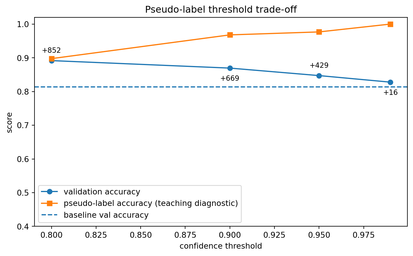
Design subtlety: the confidence threshold for accepting pseudo-labels matters.
low threshold \(\rightarrow\) more pseudo-labels, but noisier ones;
high threshold \(\rightarrow\) cleaner pseudo-labels, but fewer of them.
Higher thresholds give cleaner pseudo-labels, but far fewer of them. Lower thresholds add much more data, but with more noise. The best validation result comes from balancing those two effects.
What to notice
A good analysis is not just “semi-supervised worked” or “semi-supervised failed.”
It should say why:
lower thresholds usually add more data, but with more label noise;
higher thresholds usually add cleaner pseudo-labels, but may add too little data to matter;
validation data should choose the threshold, not the test set;
macro-F1 is worth checking because accuracy alone can hide uneven per-class behaviour.
This is exactly the kind of scientific control this course has emphasized all term.
🔬 A tiny consistency-regularization code sketch
Pseudo-labeling uses model predictions as temporary labels.
Consistency regularization instead asks the model to give similar predictions under small perturbations.
# x_u is an unlabeled minibatchp1 = model(augment(x_u)) # `augment` is stochastic. It will provide different views here.p2 = model(augment(x_u))supervised = cross_entropy(model(x_l), y_l)consistency = ((p1.softmax(dim=1) - p2.softmax(dim=1)) **2).mean()loss = supervised + lambda_u * consistencyloss.backward()optimizer.step()optimizer.zero_grad()
This does not invent hard labels.
It says: for label-preserving perturbations, predictions should be stable.
Worked example 2
Self-supervised pretraining with a denoising autoencoder
Now we switch the question.
Instead of using unlabeled data to label the task directly, we ask:
Can unlabeled data help us learn a representation that works better with very few labels?
We will:
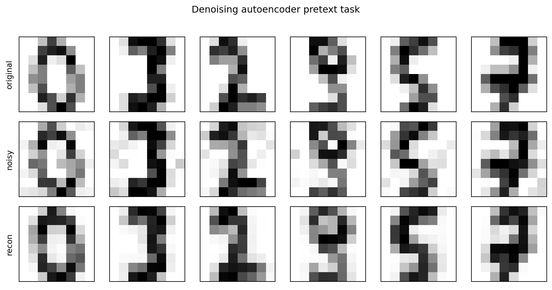
ignore labels and train a tiny denoising autoencoder on the training images;
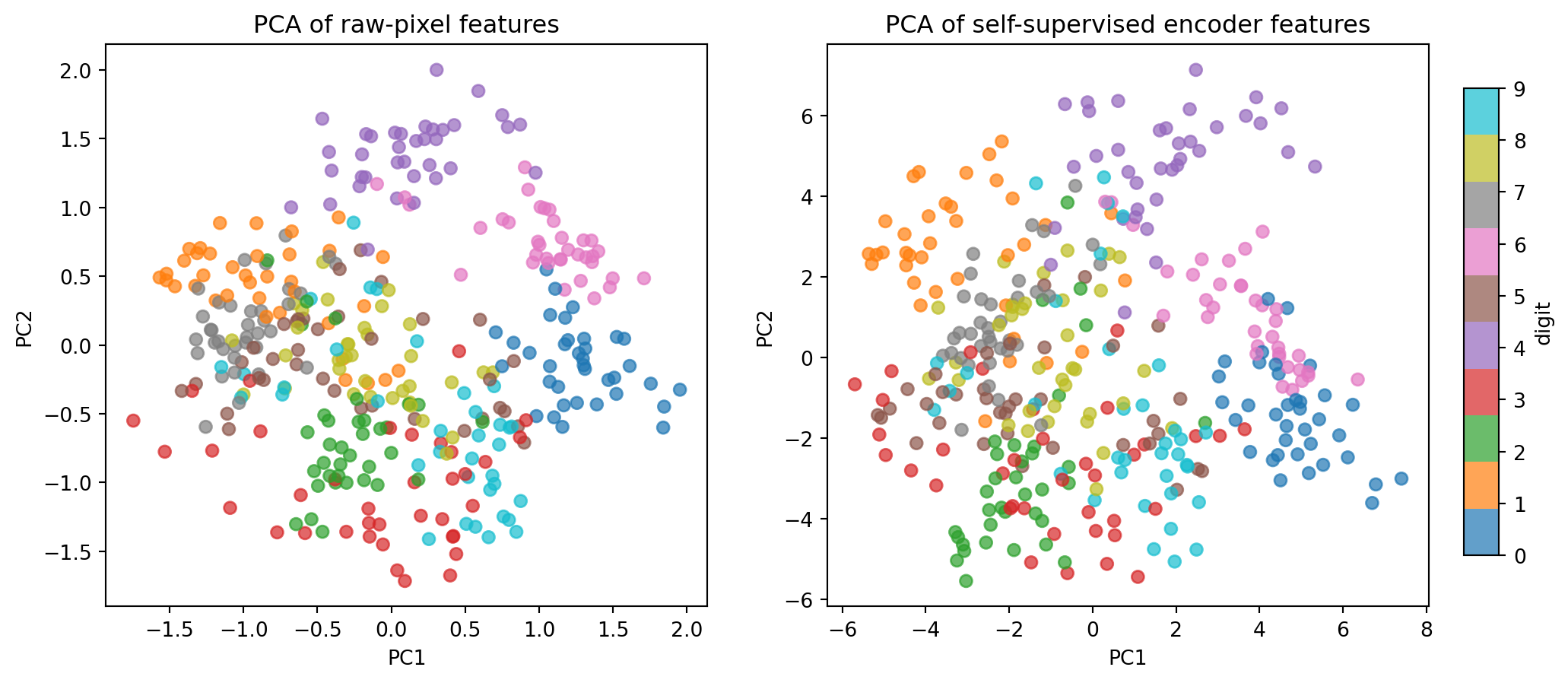
use the encoder representation as features;
fit a small supervised classifier on the same tiny labeled subset as before.
Design subtlety: the corruption strength matters.
too weak \(\rightarrow\) trivial pretext task;
too strong \(\rightarrow\) the pretext task stops matching useful structure.
the model is forced to represent stable visual structure rather than memorize a tiny labeled set;
the downstream classifier then works in a space that may already separate strokes, shapes, and local patterns;
the PCA view is only a diagnostic, but it helps us see whether the representation becomes more structured;
improvement is not guaranteed:
a poor pretext task can learn the wrong invariances;
on easy datasets, raw pixels may already be enough;
I set hidden_dim ⬆️ and latent_dim ⬆️ and noise_std ⬇️, which helped
the pretraining distribution must still resemble the downstream one.
Bird’s eye view of final thoughts
Method landscape: four patterns to know
Family
Supervision source
Typical objective
Best mental model
Main risk
Pseudo-labeling
model’s own confident predictions
add temporary labels on unlabeled data
“bootstrap the task”
confirmation of early mistakes
Consistency regularization
perturbation agreement
make predictions stable across views
“same example, same answer”
bad augmentations enforce wrong invariances
Masked prediction
hidden part of input
predict the missing piece
“fill in the blank”
pretext task may not match downstream needs
Contrastive learning
positive vs negative pairs
pull matched views together, push others apart
“who belongs with whom?”
poor pair construction or collapse
Pseudo-labeling vs consistency regularization
Both are semi-supervised, but they use unlabeled data differently.
Pseudo-labeling - turns a model prediction into a temporary hard target; - often requires a confidence threshold; - can give strong gains when predictions are already mostly correct.
Consistency regularization - does not require hard targets; - asks for stable predictions under label-preserving perturbations; - often behaves more gently early in training.
A useful rule:
pseudo-labeling says “I think this is class 3”
consistency says “I should say nearly the same thing after a small perturbation”
Masked prediction vs contrastive learning
Both are self-supervised, but they produce representations differently.
masked prediction learns from reconstruction pressure
contrastive learning learns from relative similarity pressure
Contrastive learning visual
Code
flowchart LR
    X["Example x"] --> A["Augmentation t1(x)"]
    X --> B["Augmentation t2(x)"]
    A --> ZA["Embedding z"]
    B --> ZB["Embedding z+"]
    N1["Other example"] --> ZN1["Embedding z1-"]
    N2["Other example"] --> ZN2["Embedding z2-"]

    ZA --- ZB
    ZA -. far .- ZN1
    ZA -. far .- ZN2
flowchart LR
    X["Example x"] --> A["Augmentation t1(x)"]
    X --> B["Augmentation t2(x)"]
    A --> ZA["Embedding z"]
    B --> ZB["Embedding z+"]
    N1["Other example"] --> ZN1["Embedding z1-"]
    N2["Other example"] --> ZN2["Embedding z2-"]

    ZA --- ZB
    ZA -. far .- ZN1
    ZA -. far .- ZN2
The representation should make the two views of the same item close, and views of different items relatively far apart.
wav2vec and self-supervised speech representations.
Quick checks
Q1.: A semi-supervised method is most likely to help when:
A. the unlabeled data is from a completely different population than the labeled data
B. points in dense regions tend to share labels
C. the model is already perfect on the labeled subset
D. we choose thresholds using the test set
Answer:B — semi-supervised methods often rely on cluster / low-density assumptions.
Q2. Why can a very low pseudo-label confidence threshold be dangerous?
A. it uses too little unlabeled data
B. it increases computation but never changes learning
C. it can flood training with noisy pseudo-labels
D. it guarantees overfitting
Answer:C — a low threshold adds more examples, but many may be incorrectly labeled.
Q3. A denoising autoencoder is self-supervised because:
A. it uses a human to annotate reconstructions
B. it predicts labels from a small supervised set
C. it creates a prediction task from the input itself
D. it is always trained with contrastive loss
Answer:C — the target comes from the original input, not from external labels.
Q4. You observe that self-supervised pretraining improves validation accuracy on a tiny labeled set. What is the best next check?
A. stop immediately and report only the best number
B. inspect sensitivity to pretext-task design and compare against a supervised baseline
C. add the test set into training to stabilize results
D. assume the learned representation is fair
Answer:B — we want to know whether the gain is robust and whether it comes from the intended mechanism.
References
Chen, Ting, Simon Kornblith, Mohammad Norouzi, and Geoffrey Hinton. 2020. “A Simple Framework for Contrastive Learning of Visual Representations.” In Proceedings of the 37th International Conference on Machine Learning, 119:1597–607. Proceedings of Machine Learning Research. PMLR. https://arxiv.org/abs/2002.05709.
Devlin, Jacob, Ming-Wei Chang, Kenton Lee, and Kristina Toutanova. 2019. “BERT: Pre-Training of Deep Bidirectional Transformers for Language Understanding.” In Proceedings of the 2019 Conference of the North American Chapter of the Association for Computational Linguistics: Human Language Technologies (NAACL-HLT), 4171–86.
Mnih, Volodymyr, Koray Kavukcuoglu, David Silver, Andrei A. Rusu, Joel Veness, Marc G. Bellemare, Alex Graves, et al. 2015. “Human-Level Control Through Deep Reinforcement Learning.”Nature 518 (7540): 529–33. https://doi.org/10.1038/nature14236.
Oliver, Avital, Augustus Odena, Colin Raffel, Ekin D. Cubuk, and Ian J. Goodfellow. 2018. “Realistic Evaluation of Deep Semi-Supervised Learning Algorithms.”arXiv Preprint arXiv:1804.09170. https://arxiv.org/abs/1804.09170.
Schulman, John, Filip Wolski, Prafulla Dhariwal, Alec Radford, and Oleg Klimov. 2017. “Proximal Policy Optimization Algorithms.”arXiv Preprint arXiv:1707.06347. https://arxiv.org/abs/1707.06347.
Sutton, Richard S., and Andrew G. Barto. 2018. Reinforcement Learning: An Introduction. 2nd ed. Cambridge, MA: MIT Press.
Vincent, Pascal, Hugo Larochelle, Isabelle Lajoie, Yoshua Bengio, and Pierre-Antoine Manzagol. 2010. “Stacked Denoising Autoencoders: Learning Useful Representations in a Deep Network with a Local Denoising Criterion.”Journal of Machine Learning Research 11: 3371–3408.