Any two positions interact in \(\mathcal{O}(1)\) layers.
Attention weights are interpretable diagnostics (not causal explanations).
Self-attention = query, key, and value all come from the same sequence.
Three open questions for this module:
One set of \((Q, K, V)\) weights captures one “relational pattern.” What if multiple patterns matter simultaneously?
Self-attention ignores order. How do we encode position?
How do we stack these components into a full architecture?
Each question has a well-motivated answer in the transformer.
Multi-head attention
One head, one relational pattern
Scaled dot-product attention projects the input into a single query, key, and value space and computes one weighted blend.
That means one set of linear weights determines:
which pairs of positions are “related,”
how information from one position is summarised for another.
The limitation: natural language (and many other sequences) has multiple simultaneous relationships at each position.
E.g., for the sentence “The animal didn’t cross the street because it was tired”:
“it” refers to “animal” — a coreference link
“street” and “cross” are semantically related — verb–object
“didn’t” and “cross” form a negation — grammatical
These are different kinds of dependency, active at the same position simultaneously.
Note
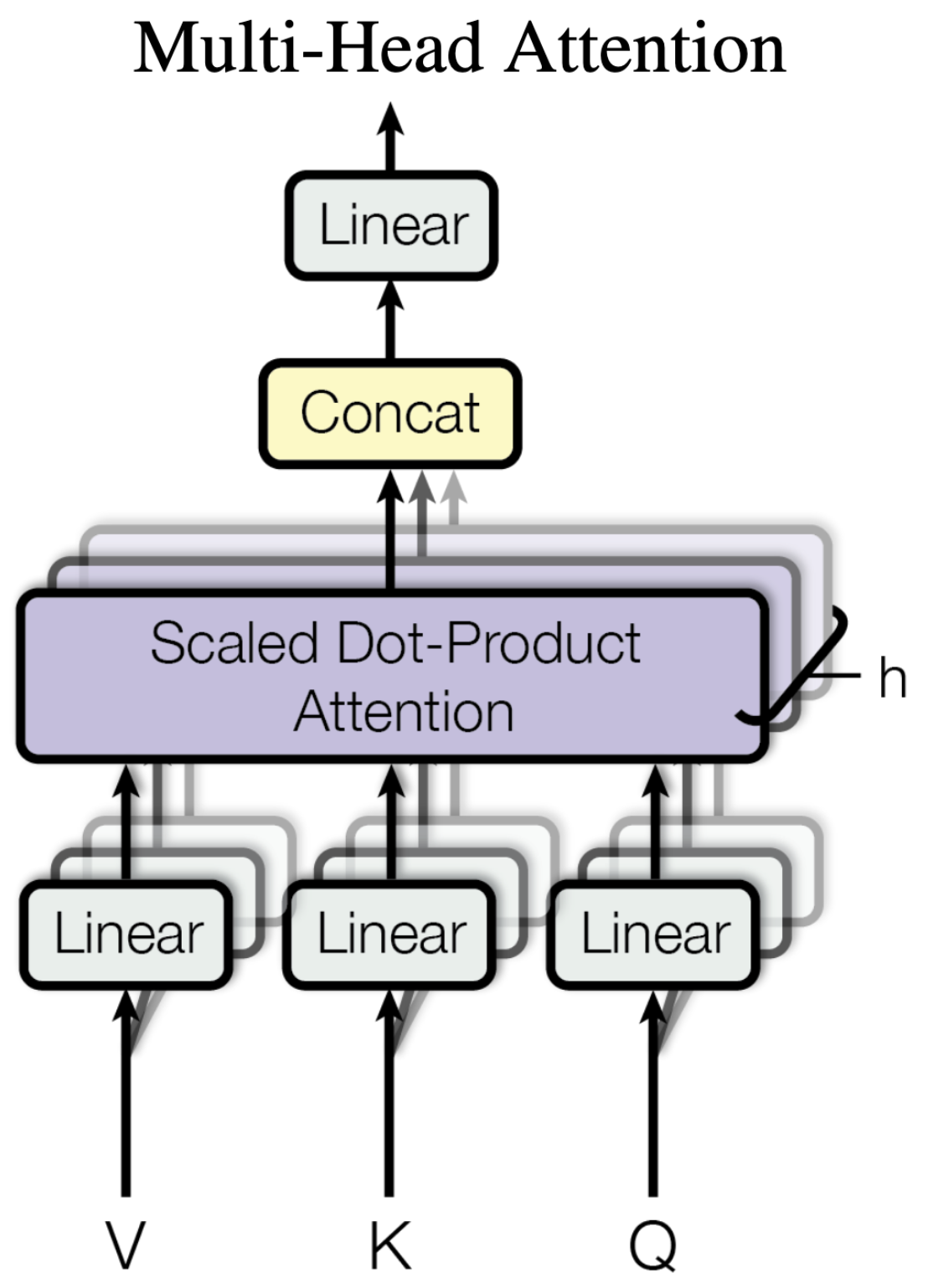
A single attention head can learn one predominant pattern well. To capture several at once, the transformer runs multiple heads in parallel — each with its own learned projections — and concatenates the results.
Multi-head attention: the idea
Run \(h\) attention heads in parallel, each with its own projection matrices.
For head \(i\):
\[
\text{head}_i = \text{Attention}(Q W_i^Q,\; K W_i^K,\; V W_i^V)
\]
Empirical observation (from Vaswani et al. (2017) and follow-up interpretability work):
Different heads in large language models tend to specialize:
some attend to nearby tokens (local syntax)
some track long-range coreference
some attend to positionally adjacent tokens
No single head does all of these well simultaneously.
(Somewhat) formal perspective:
Each head applies a different linear projection of the same input.
The model can therefore represent multiple subspaces of the interaction structure.
Concatenation merges the evidence; the output projection \(W^O\) re-mixes it.
Multi-head ≠ magic
In practice, some heads in trained models appear redundant or difficult to interpret. Head specialization is not guaranteed and varies by task and model size.
“Head pruning” experiments show many heads can be removed without significant performance loss (Michel, Levy, and Neubig 2019), suggesting the architecture provides capacity headroom, not all of which is always used.
❌️ Anti-example: why not just make \(d_k\) larger?
Tempting reasoning: if one head is limited, just increase its dimension so it has more capacity.
Why this is not the same:
Increasing \(d_k\) in a single head increases the dimension of each individual query–key comparison but still uses one set of projection weights.
The softmax over a single set of scores still collapses all relationships into one attention distribution over positions.
A single distribution cannot simultaneously give high weight to position 3 (coreference) and position 7 (verb–object) and position 2 (negation) without averaging them together.
Multi-head attention learns \(h\)separate distributions and combines them:
If you shuffle the tokens, the attention weights shuffle accordingly — but the set of output vectors is unchanged (just reordered).
This means a pure self-attention layer cannot tell “token at position 0” from “token at position 4” unless that information is somehow injected into the representations themselves.
The same token in two positions = the same representation
Without positional information, the words “dog bites man” and “man bites dog” produce the same set of token representations after one self-attention layer. For most tasks, order matters.
Sinusoidal positional encoding
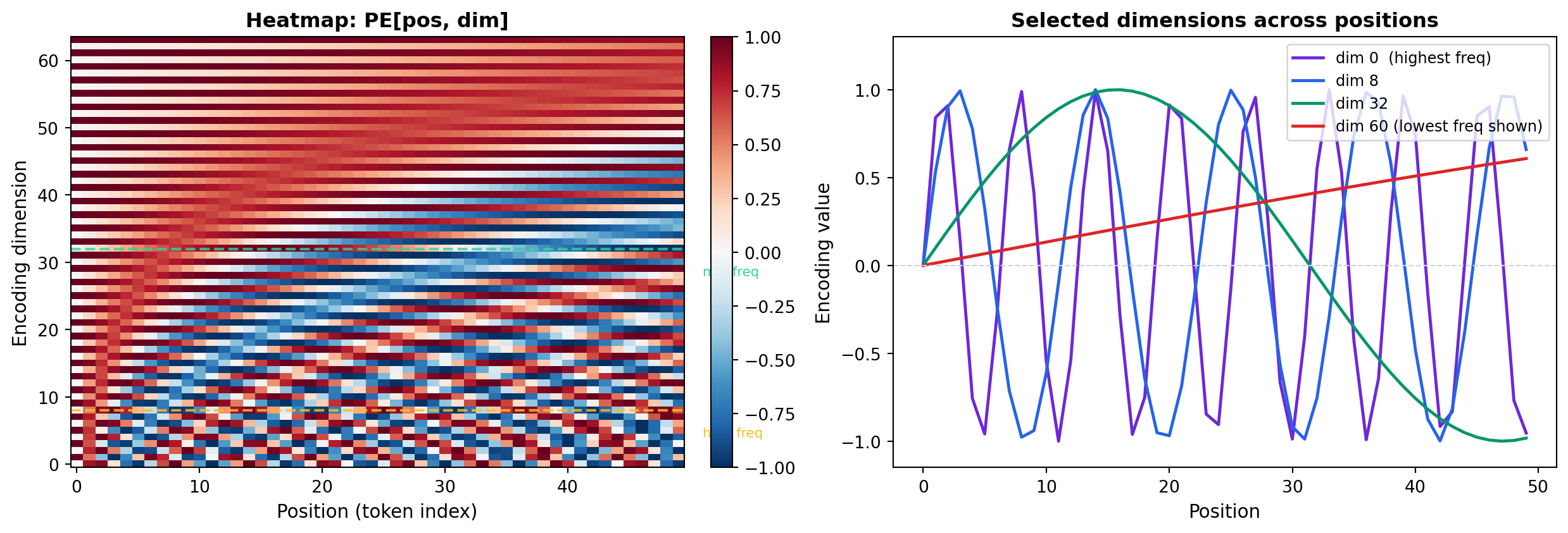
The original transformer (Vaswani et al. 2017) adds a fixed positional encoding\(PE \in \mathbb{R}^{T \times d_{\text{model}}}\) to the input embeddings before any attention.
For position \(pos \in \{0, \ldots, T-1\}\) and dimension \(2i\) or \(2i+1\):
Sinusoidal positional encodings for positions 0–49 and the first 64 dimensions of a d_model=128 model. Low-frequency (right) dimensions change slowly; high-frequency (left) dimensions change rapidly — together they form a unique fingerprint for each position.
🔬 What the encoding buys us
After adding PE to the token embeddings:
The model receives, at every token, the content of that token plus where it sits in the sequence.
Attention weights can now (implicitly) incorporate positional information via the query–key dot products.
Relative position can still be captured: the product \(PE_{pos} \cdot PE_{pos+k}\) depends only on the offset \(k\) for sinusoidal encodings — a useful inductive bias.
Learned positional embeddings are an alternative: a separate learned vector for each position (up to a maximum length). Used in BERT (Devlin et al. 2019) and many successors. More flexible, but cannot extrapolate beyond the training length.
where \(\mu, \sigma\) are computed over the \(d_{\text{model}}\) features of a single token. This works at any batch size and handles variable-length sequences naturally.
where \(y\) are the (shifted right) target embeddings and \(h^{enc}\) are the encoder outputs.
Why these three sublayers?
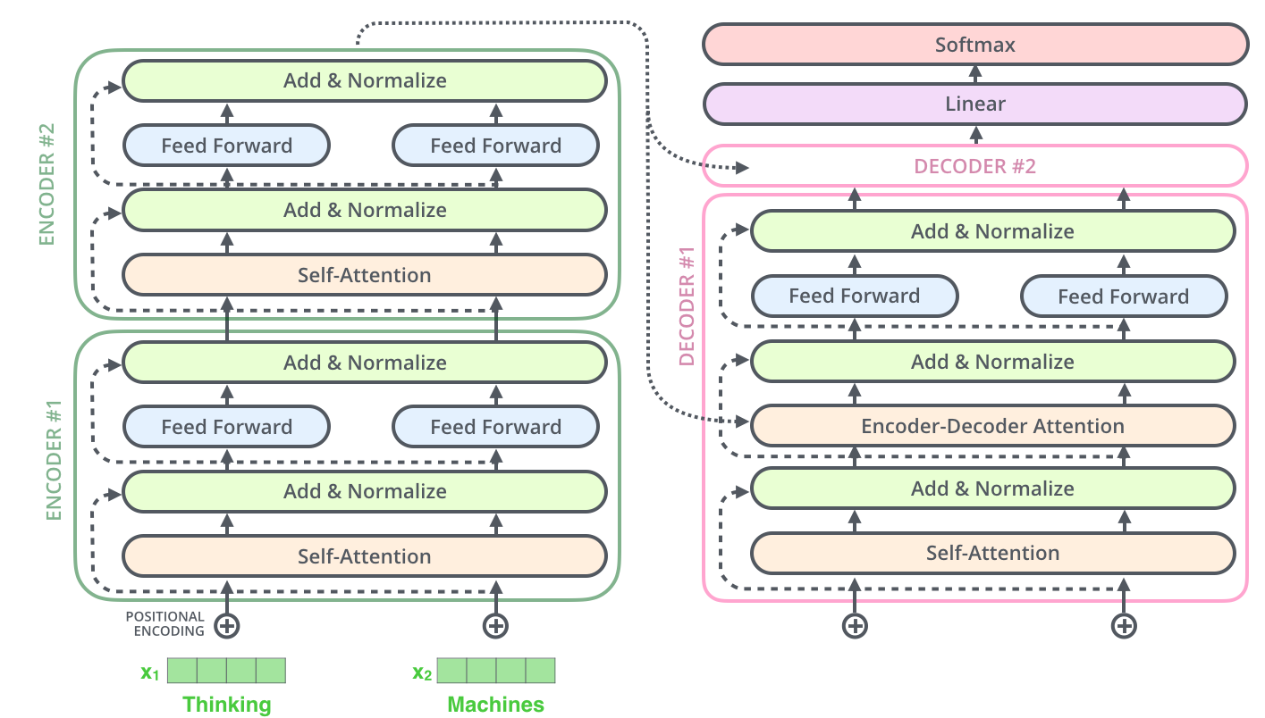
The decoder has one extra job compared to the encoder — it must both generate and condition on the source:
Masked self-attention lets each target token gather context from previously generated tokens (but not future ones).
Cross-attention connects the decoder to the encoder — the target attends to the full source representation.
The FFN re-encodes the result position-by-position, as in the encoder.
🔬 Why 😷 mask the decoder self-attention?
During training, the decoder sees the entire target sequence at once (teacher forcing: “je suis étudiant” → “i am a student”).
Without a mask, position \(t\) could attend to position \(t+1\), i.e., the decoder would see the future ground-truth tokens while predicting them.
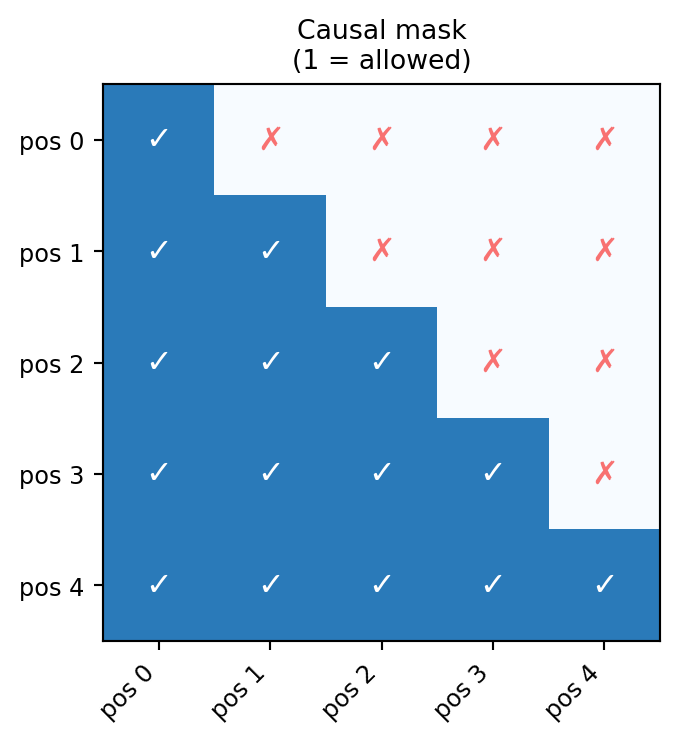
The causal (look-ahead) mask sets scores to \(-\infty\) for positions \(j > i\):
\[
M_{ij} = \begin{cases} 0 & j \le i \\ -\infty & j > i \end{cases}
\]
so after softmax, future positions receive zero weight.
At inference (autoregressive generation), there is no target sequence yet — the decoder generates one token at a time, so no masking trick is necessary.
Causal mask for a sequence of length 5. Each position can attend to itself and earlier positions only.
The encoder processes the entire source sequence in parallel; its outputs are fixed for all decoder steps. The decoder generates the target sequence autoregressively, consuming its own previous outputs.
Ablations
Not every task needs all three components; we can ablate (remove) components.
Variant
What it keeps
Typical use case
Example
Encoder-only
Encoder blocks only
Classification, tagging, embeddings
BERT
Decoder-only
Masked decoder blocks only
Language modelling, generation
GPT series
Encoder–decoder
Both
Seq-to-seq: translation, summarization, Q&A
T5, original Transformer
Design principle
If your task is understanding an existing sequence → encoder-only.
If your task is generating a sequence unconditionally → decoder-only.
If your task maps one sequence to another → encoder–decoder.
Worked examples
Example 1: positional encoding similarity
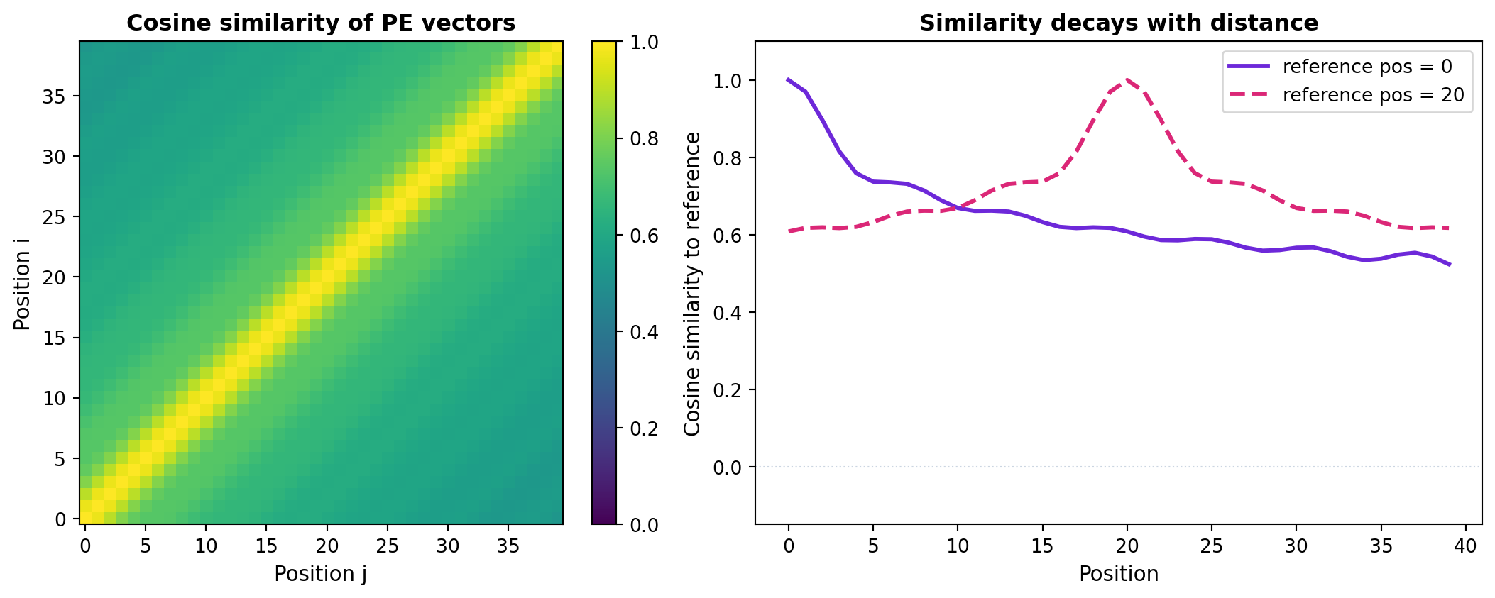
Goal: verify empirically that sinusoidal PE encodes proximity — nearby positions should have more similar encodings than distant ones.
Cosine similarity between every pair of positional encodings. The diagonal band shows that nearby positions are most similar, giving the model a sense of ‘closeness’ even before any learning.
Example 1: key design choice
What we see:
The diagonal band in the heatmap confirms that nearby positions are most similar.
Similarity from position 0 decays quickly at first then oscillates; from the midpoint it decays symmetrically in both directions.
No two positions have identical encodings (uniqueness guarantee).
Design choice:\(d_{\text{model}}\) must be large enough that the encodings are diverse.
For very small \(d\) (say, 4), the sinusoidal frequencies are coarse and many positions may end up with similar encodings.
In practice, \(d_{\text{model}} \geq 64\) gives sufficient diversity even for long sequences.
Sinusoidal PE does not prevent position confusion
A model trained on sequences of length ≤ 512 may behave unexpectedly on length 1024, because it has never seen those PE values in that combination with the data. This is one reason practitioners often cap sequence lengths or use relative position encodings (e.g., RoPE, ALiBi) in very large models.
Example 2: a small transformer encoder in PyTorch
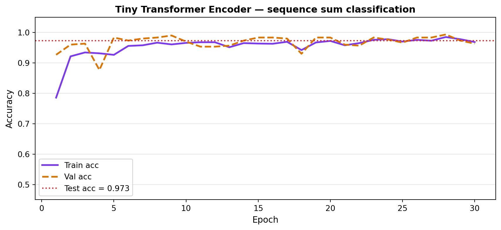
Task: classify synthetic sequences by whether the sum of tokens is above or below the median. The transformer encoder reads the whole sequence and pools to a single label.
Training and validation accuracy curves for the small transformer encoder. The model quickly learns to classify sequences by their aggregate sum, demonstrating that even two encoder layers with mean pooling can capture a global sequence property.
Final test accuracy: 0.9733
Example 2: attention pattern inspection
Code
import matplotlib.pyplot as pltimport torchmodel.eval()# Hook to capture attention weights from the first TransformerEncoderLayerattn_weights = {}def hook_fn(module, inp, out):# TransformerEncoderLayer output is just the hidden states;# we re-run attn manually for inspectionpass# Use PyTorch's built-in with need_weights=Truedef get_attn(model, x):"""Return (output, avg_attn) where avg_attn averages over heads.""" x_t = x.unsqueeze(0) # (1, T) T = x_t.size(1) emb = model.embedding(x_t) + model.pe[:, :T, :] layer = model.encoder.layers[0]# self_attn forward with need_weightswith torch.no_grad(): _, w = layer.self_attn(emb, emb, emb, need_weights=True, average_attn_weights=True)return w[0].detach().numpy() # (T, T)fig, axes = plt.subplots(1, 2, figsize=(11, 4.5))cmap ="YlOrRd"for ax, idx, prefix in [(axes[0], 0, "Example A"), (axes[1], 5, "Example B")]: x_ex = X_te[idx] w = get_attn(model, x_ex) tokens = x_ex.numpy().tolist() im = ax.imshow(w, cmap=cmap, vmin=0, vmax=2.5/T, aspect="equal") plt.colorbar(im, ax=ax, fraction=0.046, pad=0.04, label="weight") tick_pos =list(range(0, T, 2)) # every other position: 0,2,4,... ax.set_xticks(tick_pos) ax.set_xticklabels([str(p) for p in tick_pos], fontsize=8) ax.set_yticks(tick_pos) ax.set_yticklabels([str(p) for p in tick_pos], fontsize=8) ax.set_xlabel("Key position", fontsize=9) ax.set_ylabel("Query position", fontsize=9) lbl ="above"if y_te[idx].item() ==1else"below" ax.set_title(f"{prefix}: sum={sum(tokens)}, label={lbl}", fontsize=10, weight="bold")plt.suptitle("Layer-0 self-attention weights (averaged over 4 heads)", fontsize=11)plt.tight_layout()plt.show()
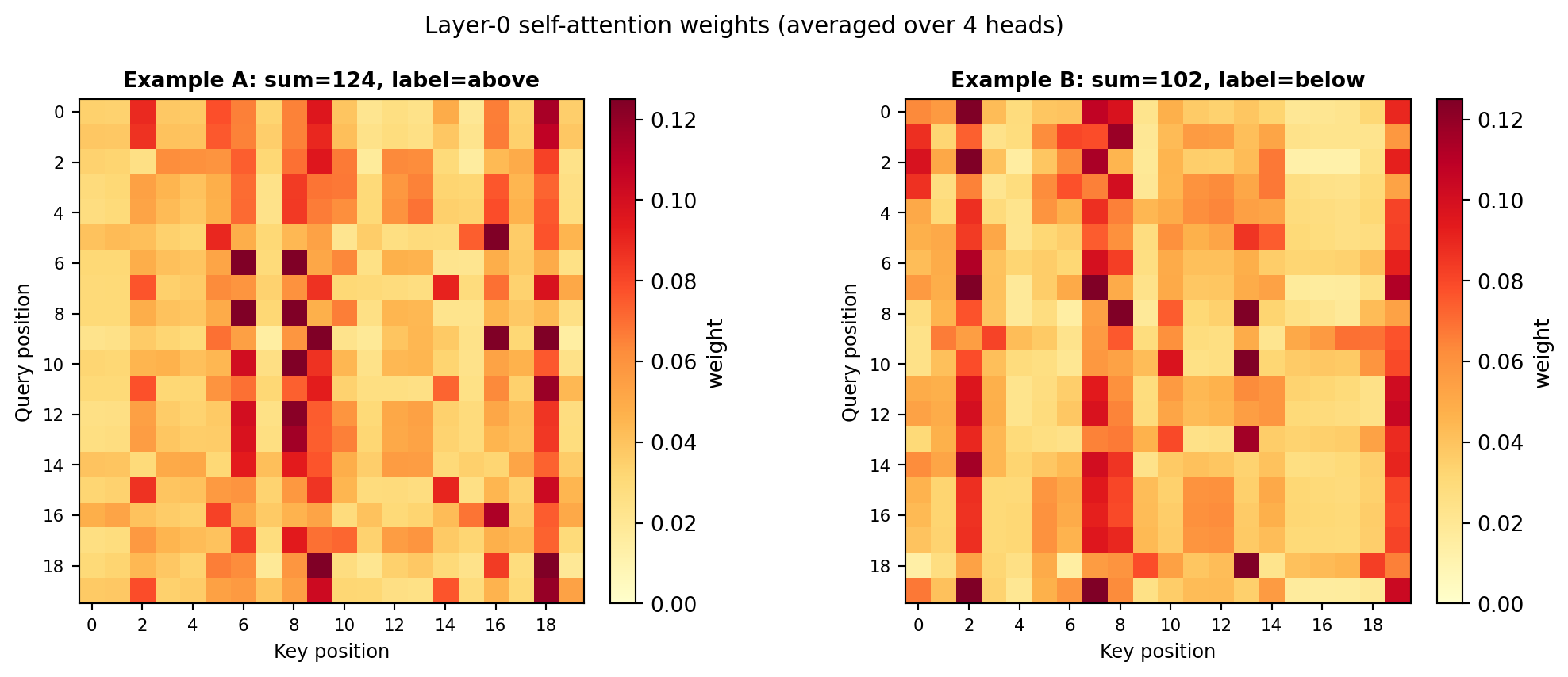
Averaged self-attention weights across all heads in layer 0, for two test sequences. Because the task depends on the sum of tokens (a global property), attention tends to spread relatively uniformly — each token needs to ‘know’ about all others.
Example 2: interpretation
What we observe:
The encoder achieves good test accuracy on this synthetic task despite having no recurrence.
Attention patterns are relatively uniform because the task requires integrating all token values — a global statistic.
Mean pooling over encoder outputs distils this global information into a single classification vector.
Two encoder layers + 4 heads are more than sufficient here; the model converges quickly.
Design choices that matter:
Positional encoding: removing it barely affects this task (sum is order-invariant), but it would matter for an order-sensitive task like “is the sequence monotonically increasing?”
Pooling strategy: mean vs [CLS] token pooling can differ; for global statistics mean pooling works well.
What this example does not show
This task is easy and well-specified. Real NLP tasks involve much longer sequences, larger vocabularies, ambiguous semantics, and pre-training requirements that a tiny from-scratch model cannot address.
The goal here is to confirm that the transformer machinery works as described — not to claim it is competitive with real language models.
🔬 parameter count in a transformer block
For a single encoder block with \(d_{\text{model}}\), \(h\) heads, and \(d_{ff}\):
🔗BERT-base has 12 such blocks: \(\approx 85M\) parameters (plus embeddings).
Note
Most parameters in a transformer live in the FFN, not in the attention mechanism.
Summary
Ethics and deployment cautions
Transformers power most modern production NLP and vision systems. The scale at which they are deployed amplifies both benefits and risks:
Bias amplification: models trained on large crawled text reproduce and reinforce stereotypes from that text. Multi-head attention does not selectively avoid stereotyped associations.
Memorization: encoder–decoder models can memorize and reproduce verbatim training sequences, including private data such as email addresses or medical text.
Environmental cost: training large transformers consumes substantial energy. Even inference is costly at deployment scale.
Misuse of cross-attention: in multimodal models, cross-attention between text and images can be exploited to produce misleading content (e.g., caption attacks, adversarial images).
Simple mitigations at a student level:
Evaluate on diverse subgroups, not just aggregate accuracy.
Prefer fine-tuning small pre-trained models over training large ones from scratch.
Inspect what training data is used before deploying a model.
Positional encoding ≠ temporal reasoning
A model that encodes position can still fail at tasks requiring genuine temporal or causal reasoning. Position encoding tells the model where a token is; it does not give the model an understanding of time, causality, or logical order.
Do not conflate architectural features with cognitive abilities.
Interpretability caution
Cross-attention heatmaps in encoder–decoder models are widely used to explain translation decisions. As with self-attention (M52), they are diagnostics, not causal explanations. Be cautious in high-stakes settings.
Why transformers changed the landscape
The original Transformer paper (Vaswani et al. 2017) introduced a set of engineering decisions that, in combination, unlocked scale:
Full parallelism — unlike RNNs, attention over the whole sequence can be computed simultaneously on GPU/TPU hardware.
\(\mathcal{O}(1)\) interaction path — any two tokens interact directly, regardless of distance.
Modular stacking — encoder and decoder blocks are similar in structure and ‘stackable’; adding more is trivially supported by the architecture.
Scalable pre-training — decoder-only transformers trained on next-token prediction at scale produce representations that transfer broadly (GPT, LLaMA).
Q1 A transformer model uses \(d_{\text{model}} = 256\) and \(h = 8\) heads. What is the standard per-head dimension \(d_k\)?
A. 256
B. 32
C. 8
D. 2048
Q2 You remove positional encoding from a transformer encoder and ask it to classify whether the sequence “1, 2, 3, 4, 5” is increasing. Which statement is most accurate?
A. Performance is unaffected because the attention mechanism inherently tracks order.
B. Performance may drop because the model cannot distinguish “1, 2, 3, 4, 5” from “3, 1, 5, 2, 4”.
C. Performance improves because less noise is added to the embeddings.
D. The model cannot be trained without positional encoding.
Q3 In the decoder of an encoder–decoder transformer, what are the queries in the cross-attention sub-layer derived from?
A. The encoder output states
B. The decoder’s own previous sub-layer output
C. The target vocabulary embeddings only
D. The positional encoding matrix
Q4 Short answer: a colleague claims “adding more attention heads always improves performance.” Give one reason this is not generally true.
Brown, Tom B., Benjamin Mann, Nick Ryder, Melanie Subbiah, Jared Kaplan, Prafulla Dhariwal, Arvind Neelakantan, et al. 2020. “Language Models Are Few-Shot Learners.” In Advances in Neural Information Processing Systems, 33:1877–1901. https://arxiv.org/abs/2005.14165.
Devlin, Jacob, Ming-Wei Chang, Kenton Lee, and Kristina Toutanova. 2019. “BERT: Pre-Training of Deep Bidirectional Transformers for Language Understanding.” In Proceedings of the 2019 Conference of the North American Chapter of the Association for Computational Linguistics: Human Language Technologies (NAACL-HLT), 4171–86.
Dosovitskiy, Alexey, Lucas Beyer, Alexander Kolesnikov, Dirk Weissenborn, Xiaohua Zhai, Thomas Unterthiner, Mostafa Dehghani, et al. 2021. “An Image Is Worth 16x16 Words: Transformers for Image Recognition at Scale.” In International Conference on Learning Representations. https://openreview.net/forum?id=YicbFdNTTy.
Han, Kai, Yunhe Wang, Hanting Chen, Xinghao Chen, Jianyuan Guo, Zhenhua Liu, Yehui Tang, et al. 2022. “A Survey on Vision Transformer.”IEEE Transactions on Pattern Analysis and Machine Intelligence 45 (1): 87–110. https://doi.org/10.1109/TPAMI.2022.3152247.
Jumper, John, Richard Evans, Alexander Pritzel, Tim Green, Michael Figurnov, Olaf Ronneberger, Kathryn Tunyasuvunakool, et al. 2021. “Highly Accurate Protein Structure Prediction with AlphaFold.”Nature 596: 583–89. https://doi.org/10.1038/s41586-021-03819-2.
Radford, Alec, Jeffrey Wu, Rewon Child, David Luan, Dario Amodei, and Ilya Sutskever. 2019. “Language Models Are Unsupervised Multitask Learners.” OpenAI. https://openai.com/blog/better-language-models.
Vaswani, Ashish, Noam Shazeer, Niki Parmar, Jakob Uszkoreit, Llion Jones, Aidan N. Gomez, Łukasz Kaiser, and Illia Polosukhin. 2017. “Attention Is All You Need.” In Advances in Neural Information Processing Systems (NeurIPS), 5998–6008. https://papers.nips.cc/paper/7181-attention-is-all-you-need.