M52: Attention Mechanisms & Self-Attention

CSCI 3151 — Foundations of Machine Learning

Frank Rudzicz

Table of contents

• Conceptual scaffold
• Math lens
• Worked example 1
• Worked example 2
• Summary

Learning outcomes

By the end of this module, you should be able to:

• explain the motivation for attention in sequence models;
• define and use queries, keys, values, scores, and attention weights;
• distinguish cross-attention from self-attention;
• compare self-attention with recurrent models;
• interpret attention patterns critically and cautiously.

From one fixed summary to selective access

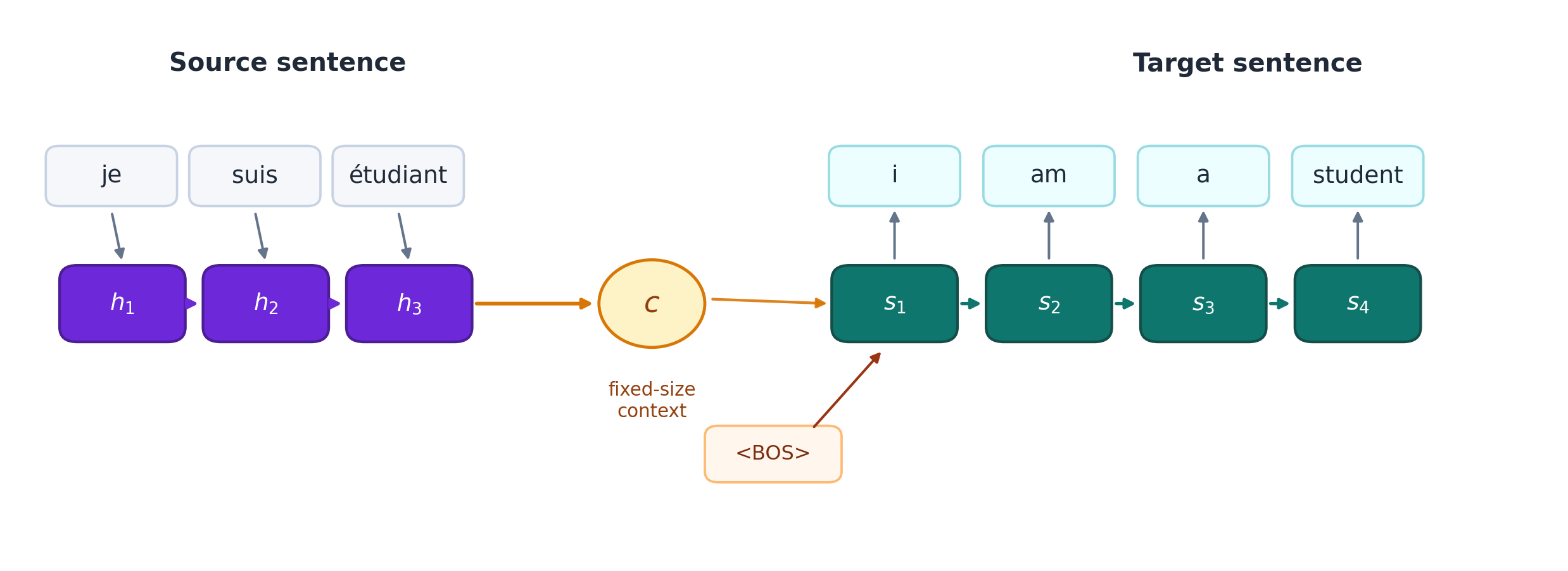
A classic use-case of encoder–decoder modelling is machine translation:

• input sequence: je suis étudiant
• output sequence: i am a student

In a vanilla encoder–decoder RNN, the encoder must compress the whole source sentence into a single fixed-size context vector.

That can work for short inputs, but it becomes a bottleneck for longer or more information-dense sequences.

So the question is:

When producing the next output token, can the decoder look back at the full source sequence instead of relying on one fixed summary?

Conceptual scaffold

Attention starts by changing the question

Recurrent view

A single rolling state must carry everything forward:

\[ h_t = f(h_{t-1}, x_t), \qquad \hat{y} = g(h_T). \]

That creates a 🍾 bottleneck:

• relevant information may be far back in the sequence,
• gradients must travel across many steps,
• different outputs may need different parts of the input.

Attention view

Instead of asking for one final summary, ask:

What does the current computation need right now, and which earlier representations are most relevant to that need?

So attention relaxes the idea that the past must be summarized once and for all.

Let the current decoding step look back at all source states

Suppose we are producing the next target token. The current decoder state should be able to consult all encoder states, not just one fixed context vector.

That means the model can decide, at each step, which source positions matter most for the current prediction.

flowchart LR
    h1(["je<br>h₁"])
    h2(["suis<br>h₂"])
    h3(["étudiant<br>h₃"])
    q(["current decoder state<br>what do I need now?"])
    h1 --> q
    h2 --> q
    h3 --> q

    style h1 fill:#ede9fe,stroke:#6d28d9,color:#111
    style h2 fill:#ede9fe,stroke:#6d28d9,color:#111
    style h3 fill:#ede9fe,stroke:#6d28d9,color:#111
    style q  fill:#ccfbf1,stroke:#0f766e,color:#111

Not all sources should matter equally

Looking back at everything is not enough; the model also needs selective focus.

For one output step, some source positions should receive larger weights than others.

That is the core intuition behind attention: compare, weight, and blend.

flowchart LR
    h1(["h₁"])
    h2(["h₂"])
    h3(["h₃"])
    q(["current need"])
    a(["attention weights<br>[0..1]"])
    c(["context vector<br>weighted blend"])

    q --> a
    h1 --> a
    h2 --> a
    h3 --> a
    a --> c

    style h1 fill:#ede9fe,stroke:#6d28d9,color:#111
    style h2 fill:#ede9fe,stroke:#6d28d9,color:#111
    style h3 fill:#ede9fe,stroke:#6d28d9,color:#111
    style q  fill:#fee2e2,stroke:#dc2626,color:#111
    style a  fill:#fef3c7,stroke:#d97706,color:#111
    style c  fill:#dcfce7,stroke:#16a34a,color:#111

High-level view: machine translation

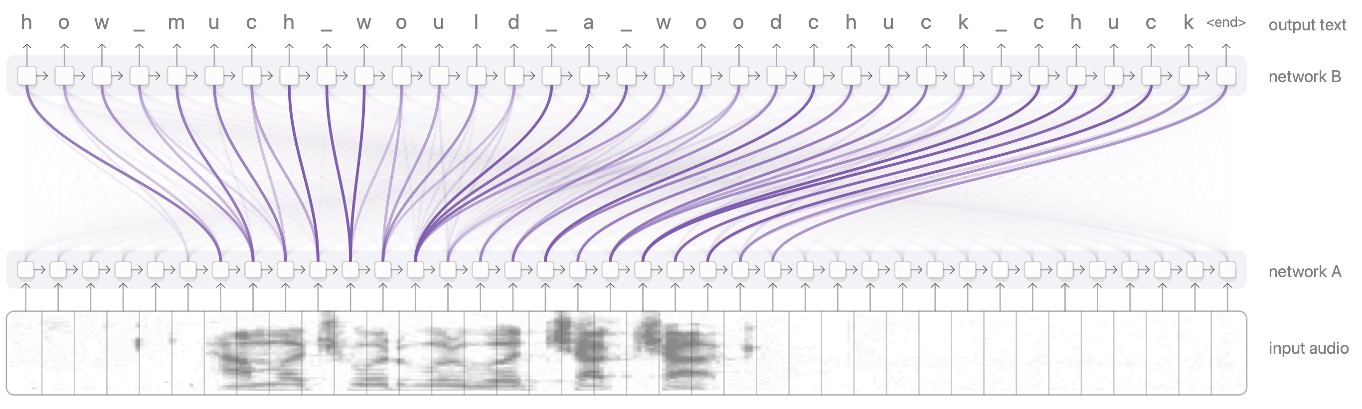
An early use of attention in RNNs was machine translation (Bahdanau, Cho, and Bengio 2014)

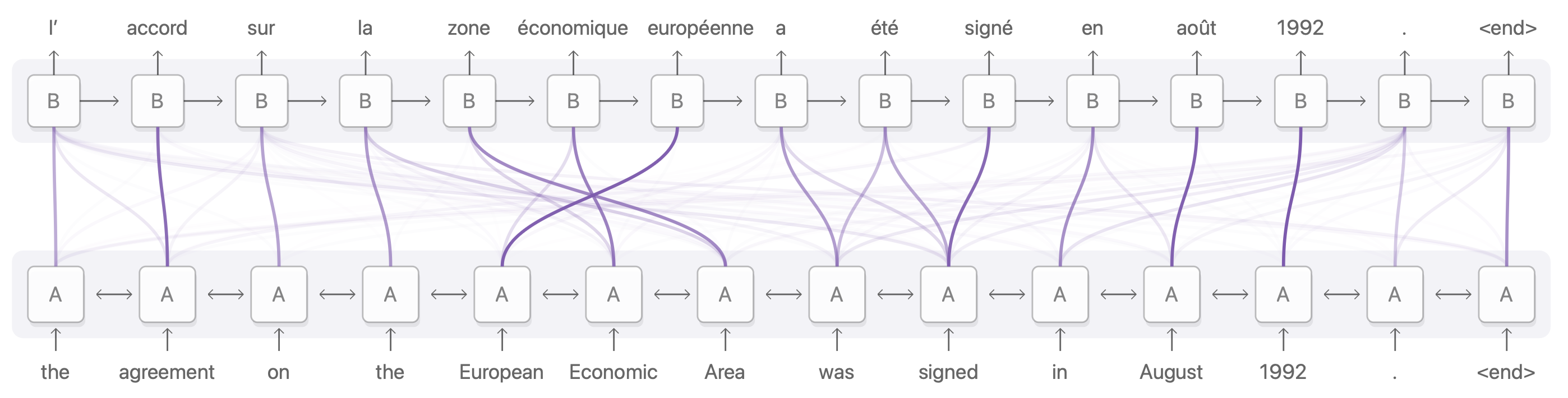
From 🔗here

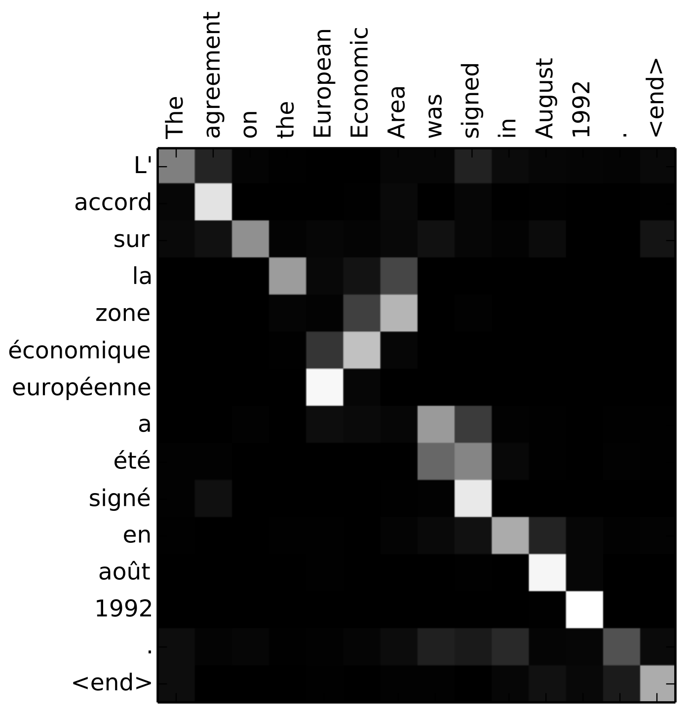
This mapping can be seen in a matrix (from Bahdanau, Cho, and Bengio (2014)):

High-level view: speech recognition

It also applies to other sequences, like acoustic frames to phonemes (Chan et al. 2015)

From 🔗here

Naming the pieces: query, keys, values

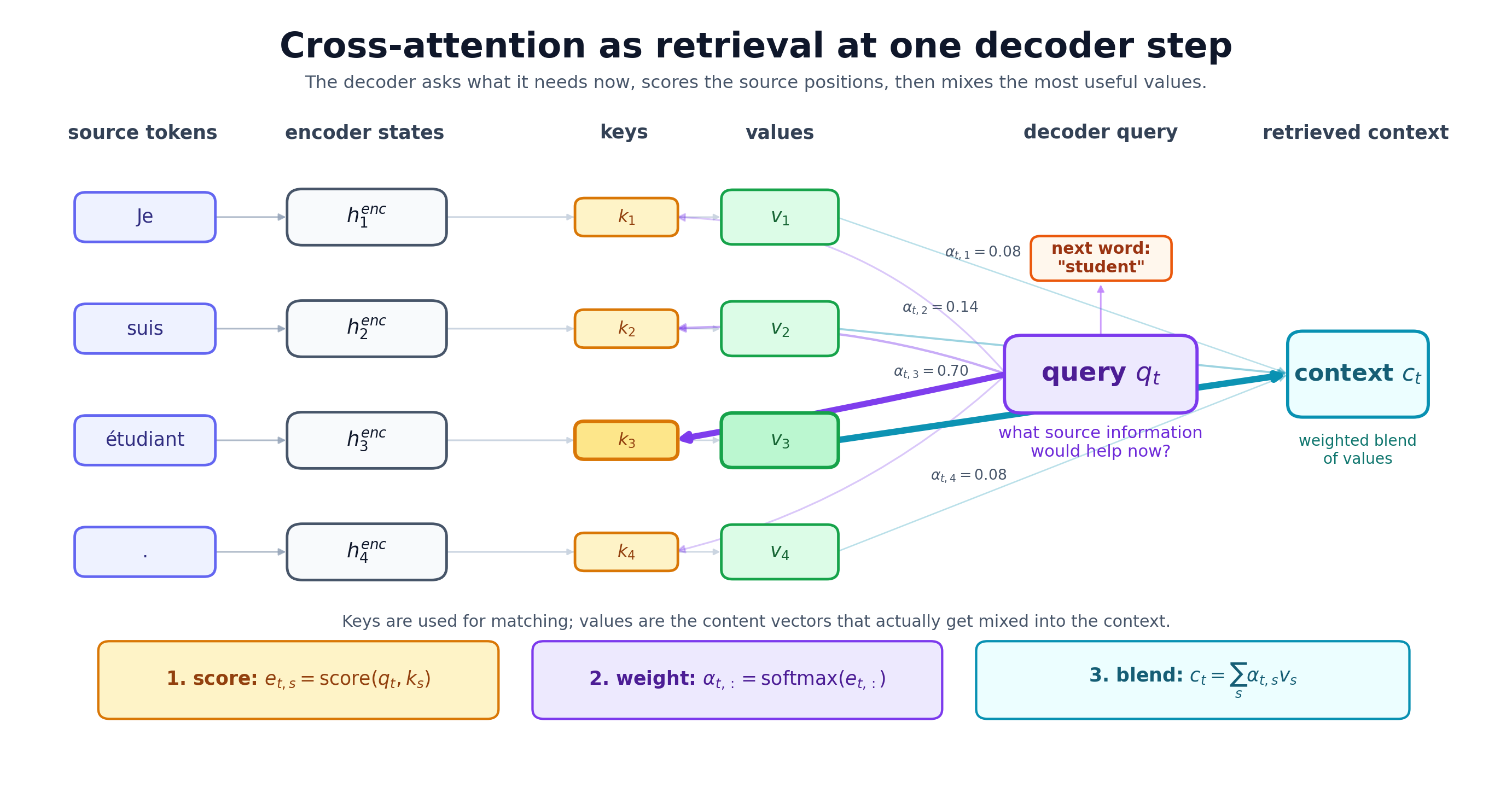
Now we can name the three roles in the mechanism:

• the query says what the current computation needs,
• the keys say where to look,
• the values say what information can be retrieved.

flowchart TB
    q(["Query<br>what am I looking for?"])

    subgraph s1["Source position 1"]
        k1(["Key 1"])
        v1(["Value 1"])
    end
    subgraph s2["Source position 2"]
        k2(["Key 2"])
        v2(["Value 2"])
    end
    subgraph s3["Source position 3"]
        k3(["Key 3"])
        v3(["Value 3"])
    end

    q --> k1
    q --> k2
    q --> k3
    v1 --> c(["context = weighted sum<br>of values"])
    v2 --> c
    v3 --> c

    style q  fill:#fee2e2,stroke:#dc2626,color:#111
    style k1 fill:#fef3c7,stroke:#d97706,color:#111
    style k2 fill:#fef3c7,stroke:#d97706,color:#111
    style k3 fill:#fef3c7,stroke:#d97706,color:#111
    style v1 fill:#dbeafe,stroke:#2563eb,color:#111
    style v2 fill:#dbeafe,stroke:#2563eb,color:#111
    style v3 fill:#dbeafe,stroke:#2563eb,color:#111
    style c  fill:#dcfce7,stroke:#16a34a,color:#111

Warning

This might be misleading. We neither ask about nor retrieve atomic facts as if from a database, but rather vectors of numbers that represent a blend of information.

Blending vectors

Suppose we have a query vector \(\color{red}{q \in \mathbb{R}^d}\), keys \(\color{orange}{k_1,\dots,k_T \in \mathbb{R}^d}\), and values \(\color{blue}{v_1,\dots,v_T \in \mathbb{R}^{d_v}}\).

A scoring function compares the query to each key:

\[ s_i = \mathrm{score}(\color{red}{q}, \color{orange}{k_i}). \]

These scores are normalized into attention weights, e.g., by:

\[ \alpha_i = \text{softmax}(s)_i = \frac{e^{s_i}}{\sum_{j=1}^T e^{s_j}}. \]

The output is a weighted sum of the values:

\[ c = \sum_{i=1}^T \alpha_i \color{blue}{v_i}. \]

🔬 Common score functions

\[ \mathrm{score}(q,k)=q^\top k \]

plain dot product

\[ \mathrm{score}(q,k)=\frac{q^\top k}{\sqrt{d_k}} \]

scaled dot product (the transformer default) (Vaswani et al. 2017)

\[ \mathrm{score}(q,k)=w^\top \tanh(W_q q + W_k k) \]

additive / Bahdanau attention (Bahdanau, Cho, and Bengio 2014)

Note

With larger \(d_k\), raw dot products become larger in magnitude, which can make the softmax too peaky. Dividing by \(\sqrt{d_k}\) keeps optimization better behaved.

Attention in one picture

Attention changes over time

Tip

Attention is not one fixed alignment for the whole sentence. The distribution changes with the output step.

current target step	Je	suis	étudiant	.	takeaway
predict am	0.10	0.72	0.13	0.05	the decoder mainly consults suis
predict student	0.08	0.14	0.70	0.08	the decoder mainly consults étudiant

Note

The same source sentence can therefore support different queries, different weights, and different retrieved contexts at different target positions.

Tradeoff: what attention helps and what it costs

Benefits ✓

• Direct access to any position — no compression bottleneck
• Better long-range relationships
• Full parallelism over sequence positions
• Flexible, content-based interactions

Costs / limits ✗

• Pairwise attention is \(\mathcal{O}(T^2)\) time and memory
• Without positional info, self-attention is permutation-equivariant (order-blind)
• Models can still learn shortcuts, spurious correlations, or memorize artifacts

Bigger is not automatically better

Larger attention models can memorize rather than generalize. Evaluation on held-out data — not attention visualizations — is what counts.

❌ Anti-example: “attention weights are the explanation”

Common misuse in practice

Attention weights are often visualized as word-importance maps. This is seductive—but not the same as a causal explanation.

Scenario:

• A model classifies a toxic comment.
• The largest attention weight falls on one identity-related word.
• We conclude: “The model based its decision only on that word, so we have a faithful explanation.”

Warning

Why this is a bad inference:

• Attention weights show one internal weighting mechanism, not necessarily a complete causal explanation.
• Different parameterizations can yield similar predictions with different attention patterns.
• Downstream nonlinear layers can transform information after attention is computed.
• See both Jain and Wallace (2019) and Wiegreffe and Pinter (2019) for two perspectives.

Tip

Better takeaway:

• Attention can be a useful diagnostic.
• It should not automatically be treated as a complete explanation of model behaviour.

Math lens

A tiny worked derivation of attention weights

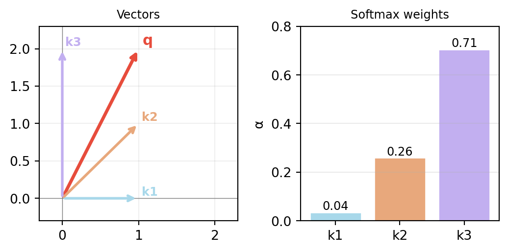
Let \(q = [1,2]^\top\) and keys:

\[ k_1 = [1,0]^\top,\; k_2 = [1,1]^\top,\; k_3 = [0,2]^\top. \]

Dot-product scores (= projection of each \(k_i\) onto \(q\)):

\[ s_1 = 1,\quad s_2 = 3,\quad s_3 = 4. \]

Softmax \(\alpha_i = e^{s_i}/(e^1+e^3+e^4)\):

The largest weight goes to \(k_3\) — it aligns most with \(q\).

Core mechanism

Similarity drives retrieval. The dot product is high when two vectors point in similar directions.

Reasoning sketch: why softmax matters

Why not just use raw scores directly?

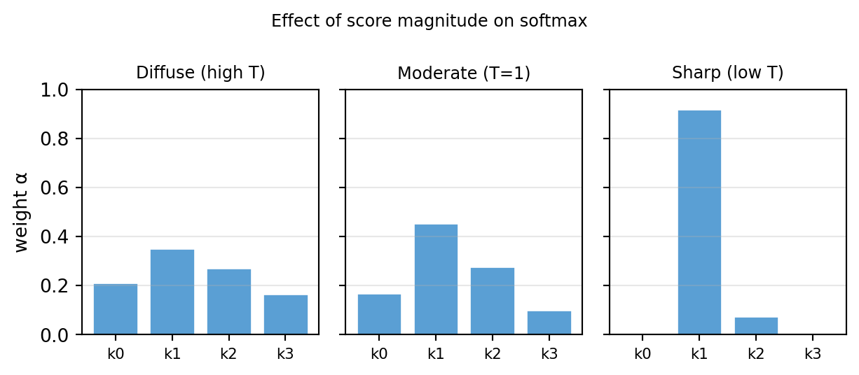
Softmax gives us:

• nonnegative weights that sum to 1
• a differentiable way to sharpen or spread focus

If one score is much larger, attention becomes concentrated. If scores are similar, attention is more diffuse.

Focus vs context

Softmax is not just normalisation — it controls the tradeoff between sharp retrieval (one position dominates) and distributed aggregation (all positions contribute).

We want relative contributions.

From cross-attention to self-attention

Cross-attention helps the decoder read the source, but it does not explain how the source representations themselves become context-aware.

🤔 So why restrict attention to decoder looking at encoder?

---

Cross-attention
(encoder–decoder attention)

A target-side state attends over source-side states:

\[ \begin{split} \begin{align} q_t &= h_t^{dec},\\ \qquad k_s &= h_s^{enc},\\ \qquad v_s &= h_s^{enc}. \end{align} \end{split} \]

Use case: connect the current output step to the most relevant input positions.

Self-attention

Every position in one sequence creates its own query, key, and value:

\[ \begin{split} \begin{align} q_i &= x_i W_Q,\\ \qquad k_i &= x_i W_K,\\ \qquad v_i &= x_i W_V. \end{align} \end{split} \]

Use case: let positions in the same sequence interact directly.

mechanism	query comes from	keys / values come from	role
cross-attention	decoder / target side	encoder / source side	link outputs to relevant inputs
self-attention	position \(i\) in a sequence	all positions in that same sequence	build contextualized token representations

Note

Cross-attention answers: which source positions help me produce the next output?
Self-attention answers: which other positions help me represent this token?

Self-attention at a single position

For token position \(i\), self-attention computes

\[ \begin{split} e_{ij} = \frac{q_i^\top k_j}{\sqrt{d_k}}, \qquad \alpha_{ij} = \operatorname{softmax}(e_{i,:})_j,\\ \qquad z_i = \sum_j \alpha_{ij} v_j. \end{split} \]

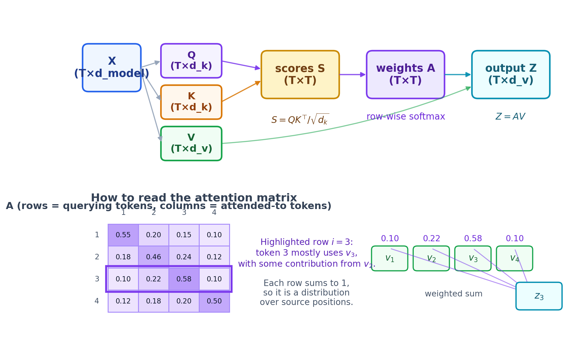
So row \(i\) of the attention matrix is a probability distribution over which positions token \(i\) consults.

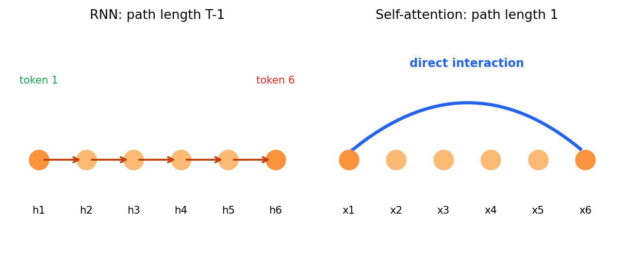
That is the key shift from recurrent models: position \(i\) does not need to wait for information to be passed along one step at a time.

flowchart LR
    q(["query from token i<br>q_i"])
    k1(["k_1, v_1"])
    k2(["k_2, v_2"])
    k3(["k_3, v_3"])
    k4(["k_4, v_4"])
    a(["weights<br>α_i1 ... α_i4"])
    z(["updated token<br>representation z_i"])

    q --> a
    k1 --> a
    k2 --> a
    k3 --> a
    k4 --> a
    a --> z

    style q fill:#ede9fe,stroke:#7c3aed,color:#111
    style k1 fill:#dbeafe,stroke:#2563eb,color:#111
    style k2 fill:#dbeafe,stroke:#2563eb,color:#111
    style k3 fill:#dbeafe,stroke:#2563eb,color:#111
    style k4 fill:#dbeafe,stroke:#2563eb,color:#111
    style a fill:#fef3c7,stroke:#d97706,color:#111
    style z fill:#dcfce7,stroke:#16a34a,color:#111

🔬 Self-attention in matrix form

Stack the token vectors row-wise into \[ X \in \mathbb{R}^{T\times d_{model}}. \] Then compute all queries, keys, and values in parallel: \[ \begin{split} \begin{align} Q &= XW_Q,\\ \qquad K&=XW_K,\\ \qquad V&=XW_V. \end{align} \end{split} \] For one head, \[ \begin{split} \begin{align} S &= \frac{QK^\top}{\sqrt{d_k}},\\ \qquad A &= \operatorname{row\text{-}softmax}(S),\\ \qquad Z &= AV. \end{align} \end{split} \]

What each matrix means

• \(S\in\mathbb{R}^{T\times T}\): raw pairwise compatibility scores.
• \(A\in\mathbb{R}^{T\times T}\): attention weights after a row-wise softmax.
• \(Z\in\mathbb{R}^{T\times d_v}\): updated, context-aware token representations.

For token \(i\), \[ \begin{split} \begin{align} A_{ij} = &\text{how much token } i\\ & \text{ attends to token } j, \end{align} \end{split} \] so the new representation is \[ z_i = \sum_{j=1}^T A_{ij}v_j. \] That is: row \(i\) of \(A\) is the retrieval distribution used to update token \(i\).

Why this was a big deal for sequence modelling

With recurrence

• information is compressed into a rolling hidden state,
• token 1 influences token \(T\) only after \(T-1\) chained transitions,
• computation is inherently sequential.

With self-attention

• any position can interact with any other position in one layer,
• long-range dependencies have much shorter paths,
• all positions can be processed in parallel.

Note

This is one reason attention works well for long-range structure: the model does not need to preserve every useful signal through a long chain of recurrent updates before it can be used.

Positions: order is not free

Pure self-attention compares content vectors; by itself, it does not know whether a token came first, last, or in the middle.

Note

That matters because order changes meaning:

• dog bites man
• man bites dog

contain the same words but encode different relationships.

So transformer models must add positional information explicitly, e.g., through

• learned positional embeddings,
• sinusoidal positional encodings,
• relative-position mechanisms.

Note

Self-attention is powerful because it is flexible; positional encoding is necessary because language is ordered.

M53 can then pick up naturally from here by formalizing how transformer blocks combine self-attention with positional information.

🔬 Computational comparison with recurrent models

Very roughly, for sequence length \(T\) and hidden width \(d\) (Vaswani et al. 2017):

• recurrent layer: often \(\mathcal{O}(Td^2)\), sequential over time
• self-attention layer: often \(\mathcal{O}(T^2 d)\) for dense attention over all token pairs

So self-attention replaces sequential dependence with denser pairwise interaction.

Note

This is one reason transformers excel on moderate-length sequences with parallel hardware, while also motivating later research on sparse, linear, or chunked attention for very long contexts (Tay et al. 2020).

Worked example 1

Computing and visualizing attention on a toy sentence

Goal:

• build query–key–value attention on a short token sequence
• inspect the resulting attention weights as both a table and a figure
• identify the design choice of where the query comes from

QKV computation step by step

import numpy as np
import pandas as pd
import matplotlib.pyplot as plt

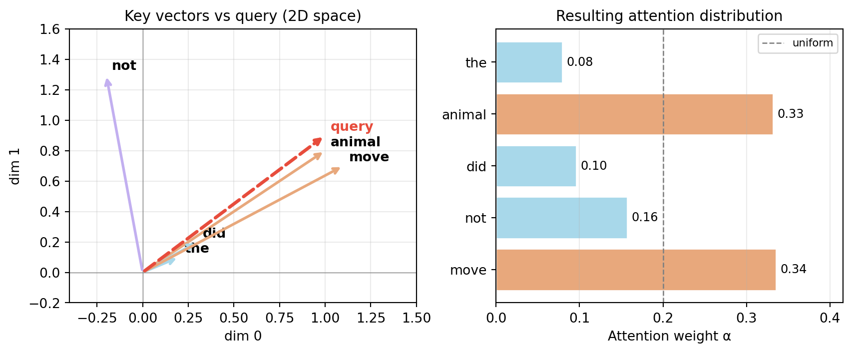
tokens = ["the", "animal", "did", "not", "move"]

# 2D toy embeddings (chosen for clear geometric interpretation)
X = np.array([
    [0.2, 0.1],   # the  — function word, low content
    [1.0, 0.8],   # animal — content noun
    [0.3, 0.2],   # did  — function word
    [-0.2, 1.3],  # not  — negation, distinctive direction
    [1.1, 0.7],   # move — action verb, similar to animal
])

# Query: "what matters for deciding whether action occurred?"
q = np.array([1.0, 0.9])
K = X.copy()   # keys  = same as embeddings in this toy
V = X.copy()   # values = same

scores  = K @ q                                # raw dot-product scores
weights = np.exp(scores) / np.exp(scores).sum()  # softmax
context = weights @ V                          # weighted sum of values

pd.DataFrame({
    "token":  tokens,
    "score":  np.round(scores, 3),
    "α (weight)": np.round(weights, 3),
}).sort_values("α (weight)", ascending=False)

	token	score	α (weight)
4	move	1.73	0.335
1	animal	1.72	0.332
3	not	0.97	0.157
2	did	0.48	0.096
0	the	0.29	0.079

Geometry + weights

Left: query vs key vectors in 2D space (dot-product = projection onto query). Right: resulting attention weights.

Interpretation

What to notice:

• The query aligns most strongly with content-like tokens such as animal and move.
• Function words like the and did receive smaller weights.
• The context vector is a weighted blend, not a hard pointer.

Subtle design choice:

• If we changed the query, we would change what the model retrieves.
• Attention is therefore task-conditional: what matters depends on the current prediction.

Anti-example connected to this code:

• Do not interpret the largest weight as “the only token that matters.”
• Multiple moderately weighted tokens may jointly shape the output.

Worked example 2

GRU vs self-attention on a synthetic long-range task

Task:

• Input: a sequence of integer tokens of length 30
• Label: 1 if the first and last token match, else 0

Why this is useful:

• the decisive information is at two distant positions
• a sequential recurrent summary may learn this, but the architectural path is longer
• a self-attention model can compare distant positions more directly

Design subtlety:

• This task is synthetic and intentionally narrow; it isolates an architectural issue rather than representing realistic language understanding.

Run the experiment

import numpy as np
import pandas as pd
import matplotlib.pyplot as plt
import torch
import torch.nn as nn
from torch.utils.data import TensorDataset, DataLoader
from sklearn.metrics import accuracy_score, confusion_matrix, ConfusionMatrixDisplay

rng = np.random.default_rng(3151)
torch.manual_seed(3151)

VOCAB  = 8
T      = 30   # sequence length — long enough to stress RNN memory
d_model = 16

def make_balanced(n, seq_len=T, vocab=VOCAB):
    """Exactly 50% positive (first == last), 50% negative."""
    X = rng.integers(0, vocab, size=(n, seq_len))
    half = n // 2
    X[:half, -1] = X[:half, 0]          # positive: force last = first
    for i in range(half, n):             # negative: force last ≠ first
        v = X[i, -1]
        while v == X[i, 0]:
            v = rng.integers(0, vocab)
        X[i, -1] = v
    y   = (X[:, 0] == X[:, -1]).astype(np.int64)
    idx = rng.permutation(n)
    return X[idx], y[idx]

X_tr, y_tr = make_balanced(2400)
X_va, y_va = make_balanced(600)
X_te, y_te = make_balanced(600)

tr_loader = DataLoader(TensorDataset(torch.tensor(X_tr), torch.tensor(y_tr)),
                       batch_size=64, shuffle=True)
va_loader = DataLoader(TensorDataset(torch.tensor(X_va), torch.tensor(y_va)), batch_size=512)
te_loader = DataLoader(TensorDataset(torch.tensor(X_te), torch.tensor(y_te)), batch_size=512)

class GRUClassifier(nn.Module):
    def __init__(self, vocab=VOCAB, d_model=16, hidden=20):
        super().__init__()
        self.emb = nn.Embedding(vocab, d_model)
        self.gru = nn.GRU(d_model, hidden, batch_first=True)
        self.fc  = nn.Linear(hidden, 2)
    def forward(self, x):
        e = self.emb(x)
        _, h = self.gru(e)
        return self.fc(h[-1])

class TinySelfAttn(nn.Module):
    def __init__(self, vocab=VOCAB, d_model=16):
        super().__init__()
        self.emb = nn.Embedding(vocab, d_model)
        self.pos = nn.Embedding(T, d_model)
        self.Wq  = nn.Linear(d_model, d_model, bias=False)
        self.Wk  = nn.Linear(d_model, d_model, bias=False)
        self.Wv  = nn.Linear(d_model, d_model, bias=False)
        self.fc  = nn.Linear(d_model, 2)
    def forward(self, x, return_attn=False):
        B, T = x.shape
        positions = torch.arange(T).unsqueeze(0).expand(B, -1)
        e = self.emb(x) + self.pos(positions)
        Q, K, V = self.Wq(e), self.Wk(e), self.Wv(e)
        A = torch.softmax(Q @ K.transpose(1, 2) / (Q.shape[-1]**0.5), dim=-1)
        Z = (A @ V)[:, -1, :]
        # Z = (A @ V).mean(dim=1)
        logits = self.fc(Z)
        return (logits, A) if return_attn else logits

def evaluate(model, loader):
    model.eval(); ys, ps = [], []
    with torch.no_grad():
        for xb, yb in loader:
            ps.extend(model(xb).argmax(1).numpy()); ys.extend(yb.numpy())
    return accuracy_score(ys, ps)

def train_model(model, epochs=35, lr=5e-3):
    opt     = torch.optim.Adam(model.parameters(), lr=lr)
    loss_fn = nn.CrossEntropyLoss()
    hist    = []
    for ep in range(1, epochs + 1):
        model.train()
        for xb, yb in tr_loader:
            opt.zero_grad()
            loss_fn(model(xb), yb).backward()
            opt.step()
        tr_acc = evaluate(model, tr_loader)
        va_acc = evaluate(model, va_loader)
        hist.append({"epoch": ep, "train_acc": tr_acc, "val_acc": va_acc})
    return pd.DataFrame(hist)

gru_model  = GRUClassifier()
attn_model = TinySelfAttn()

gru_hist  = train_model(gru_model,  epochs=35)
attn_hist = train_model(attn_model, epochs=35)

summary = pd.DataFrame([
    {"model": "GRU",              "test_acc": evaluate(gru_model,  te_loader)},
    {"model": "Tiny self-attn",   "test_acc": evaluate(attn_model, te_loader)},
]).round(3)
summary

	model	test_acc
0	GRU	0.485
1	Tiny self-attn	1.000

Note!

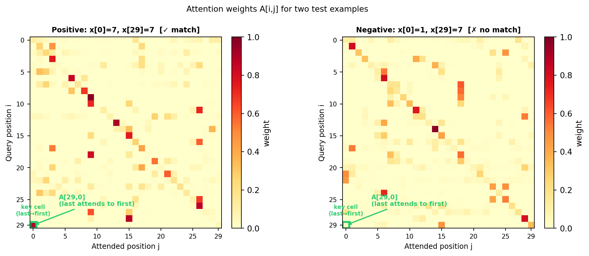
This example encodes the positions which attention mechanisms don’t do by default. We’re getting ahead of ourselves a bit.

Learning curves on the fixed task

In this run and on this toy task, both models start near chance (50%). Self-attention converges faster; the GRU performs worse because it must preserve the first-token signal across 29 recurrent updates.

A diagnostic look at the learned attention

Self-attention weight matrices A[i,j] for a positive example (first==last, left) and a negative example (first≠last, right). For this task, one useful pattern is for the last position to place weight on the first position, since comparing x[29] with x[0] helps determine the label.

Interpretation

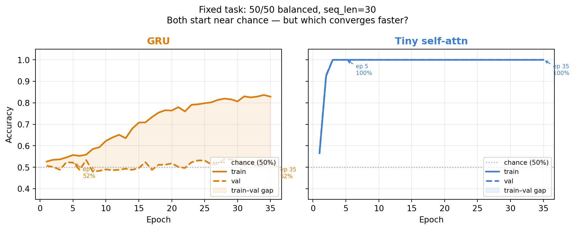
What we see in this single toy setup:

• Both models start near 50% (chance) — the task genuinely requires learning
• The tiny self-attention model quickly learns the endpoint-comparison task.
• Self-attention converges faster because position 0 and position 29 can interact directly in one layer
• The GRU struggles here. It must compress the first-token signal through 29 recurrent updates before it is available to the classifier
• This is consistent with the idea that attention provides a shorter interaction path between distant positions.

What to be cautious about:

• This is a narrow synthetic task isolating one architectural difference
• On real language data, GRUs (and LSTMs) can work well with enough capacity
• Self-attention’s \(O(T^2)\) cost means it is not always the right choice for very long sequences

The core lesson

Self-attention reduces the interaction path length between any two positions from \(\mathcal{O}(T)\) (RNN) to \(\mathcal{O}(1)\) (Vaswani et al. 2017). For tasks that require comparing distant positions, this architectural shortcut speeds up learning.

What this task does not show

Accuracy on this synthetic benchmark does not mean a model “understands” sequences. It shows one specific architectural property — direct positional comparison — under controlled conditions.

What could still go wrong?

Even if metrics look good:

• a model may overfit sequence length or token frequency quirks
• attention plots may look plausible but not be robust
• a toy architecture may fail on variable-length or noisier real data
• training may depend strongly on initialization, width, or pooling choice

Note

This is part of the course theme: architecture, objective, and evaluation must be aligned.

Summary

Ethics and deployment cautions

If attention-based models are used on real language or user data, several risks appear immediately:

• Bias amplification: large text corpora contain stereotypes; attention does not remove them
• Privacy leakage: models may memorize rare phrases or sensitive patterns
• Misleading interpretability: stakeholders over-trust attention heatmaps as causal explanations
• Shortcut learning: models attend to superficial cues rather than the intended signal

Attention ≠ explanation

Visualizing attention weights has become a default way to “explain” model decisions. Research shows this can be misleading: adversarially constructed attention patterns can give the same predictions with very different distributions (Jain and Wallace 2019; Serrano and Smith 2019).

Always pair attention diagnostics with behavioural evaluation (e.g., stress tests, subgroup performance, counterfactual inputs).

Why attention mattered historically

• Before transformers dominated, encoder–decoder RNNs for machine translation often struggled because the decoder had to rely on a single compressed encoder summary.
  • Attention changed that by letting the decoder revisit different source words at different decoding steps.

This was a conceptual shift (although very similar to IBM alignment models (Brown et al. 1993)):

• from “remember everything in one state”
• to “store many representations and retrieve what matters now”

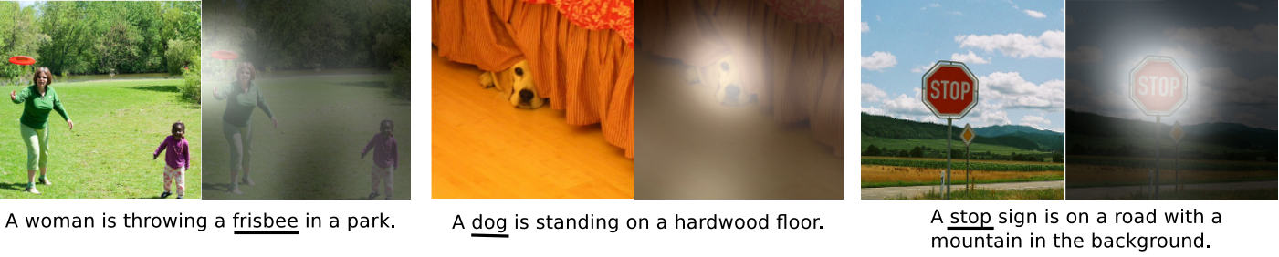
That idea generalizes well beyond translation.

Beyond text: attention everywhere

Attention and self-attention appear in:

• Language — language models, chat systems, machine translation
• Vision — Vision Transformers (ViT) treat image patches as tokens
• Speech — recognition and audio tagging
• Multimodal — systems linking text, images, and audio
• Retrieval-augmented — internal attention + external memory

From Xu et al. (2015)

Looking ahead to M53

This module gave the central mechanism:

• query–key–value attention
• cross-attention vs self-attention
• self-attention as token-to-token interaction
• strengths and tradeoffs relative to recurrence

Next module:

• multi-head attention
• positional encoding
• feedforward sublayers, residual connections, layer normalization
• encoder–decoder structure and transformer blocks

Quick checks

Q1 A model uses self-attention over a sequence but does not include any positional information. Which statement is best?

A. The model automatically knows token order from the softmax. B. The model can still compare content, but order information is not explicitly encoded. C. The model becomes identical to an LSTM. D. The model cannot be trained with gradient descent.

Q2 Suppose a query gives scores \([0, 2, 2]\) over three keys. After softmax, which is true?

A. The first key gets the largest weight. B. The second and third keys receive equal weights larger than the first. C. All three keys receive equal weight. D. Softmax cannot be applied because of repeated scores.

Q3 Why can self-attention help with long-range dependencies relative to a vanilla RNN?

Write 1–2 sentences.

Q4 You train a text classifier and show an attention heatmap where one word receives the highest weight. What is the safest conclusion?

A. That word is the full causal explanation of the prediction. B. The model ignored all other words. C. The heatmap is one useful diagnostic, but not automatically a complete explanation. D. The model is unbiased because the heatmap looks sparse.

References

Bahdanau, Dzmitry, Kyunghyun Cho, and Yoshua Bengio. 2014. “Neural Machine Translation by Jointly Learning to Align and Translate.” arXiv Preprint arXiv:1409.0473. https://arxiv.org/abs/1409.0473.

Brown, Peter F., Stephen A. Della Pietra, Vincent J. Della Pietra, and Robert L. Mercer. 1993. “The Mathematics of Statistical Machine Translation: Parameter Estimation.” Computational Linguistics 19 (2): 263–311. https://aclanthology.org/J93-2003/.

Chan, William, Navdeep Jaitly, Quoc V. Le, and Oriol Vinyals. 2015. “Listen, Attend and Spell.” CoRR abs/1508.01211. http://arxiv.org/abs/1508.01211.

Jain, Sarthak, and Byron C. Wallace. 2019. “Attention Is Not Explanation.” In Proceedings of the 2019 Conference of the North American Chapter of the Association for Computational Linguistics: Human Language Technologies, Volume 1 (Long and Short Papers), 3543–56. Minneapolis, Minnesota: Association for Computational Linguistics. https://doi.org/10.18653/v1/N19-1357.

Serrano, Sofia, and Noah A. Smith. 2019. “Is Attention Interpretable?” In Proceedings of the 57th Annual Meeting of the Association for Computational Linguistics, 2931–51. Florence, Italy: Association for Computational Linguistics. https://doi.org/10.18653/v1/P19-1282.

Tay, Yi, Mostafa Dehghani, Dara Bahri, and Donald Metzler. 2020. “Efficient Transformers: A Survey.” arXiv Preprint arXiv:2009.06732. https://arxiv.org/abs/2009.06732.

Vaswani, Ashish, Noam Shazeer, Niki Parmar, Jakob Uszkoreit, Llion Jones, Aidan N. Gomez, Łukasz Kaiser, and Illia Polosukhin. 2017. “Attention Is All You Need.” In Advances in Neural Information Processing Systems (NeurIPS), 5998–6008. https://papers.nips.cc/paper/7181-attention-is-all-you-need.

Wiegreffe, Sarah, and Yuval Pinter. 2019. “Attention Is Not Not Explanation.” In Proceedings of the 2019 Conference on Empirical Methods in Natural Language Processing and the 9th International Joint Conference on Natural Language Processing (EMNLP-IJCNLP), 11–20. Hong Kong, China: Association for Computational Linguistics. https://doi.org/10.18653/v1/D19-1002.

Xu, Kelvin, Jimmy Lei Ba, Ryan Kiros, Kyunghyun Cho, Aaron Courville, Ruslan Salakhutdinov, Richard Zemel, and Yoshua Bengio. 2015. “Show, Attend and Tell: Neural Image Caption Generation with Visual Attention.” In Proceedings of the 32nd International Conference on Machine Learning, edited by Francis Bach and David Blei, 37:2048–57. Proceedings of Machine Learning Research. Lille, France: PMLR.