M49: LSTMs, GRUs, and Gated RNN Variants

CSCI 3151 — Foundations of Machine Learning

Frank Rudzicz

Learning outcomes

By the end of this module, you should be able to:

  1. Explain the role of each LSTM gate (forget, input, output) and the cell state, using both equations and plain language.
  2. Derive how the LSTM cell state update provides an additive gradient pathway that mitigates vanishing gradients.
  3. Compare LSTM and GRU architectures — parameter counts, gating structure, and typical empirical tradeoffs.
  4. Implement LSTM and GRU models in PyTorch and diagnose their behaviour on a controlled long-range dependency task.
  5. Justify the choice between vanilla RNN, LSTM, and GRU for a given sequence modelling setting using evidence from learning curves and validation performance.

Conceptual scaffold

Core problem: a single vector does too much

In a vanilla RNN, the hidden state \(\mathbf{h}_t \in \mathbb{R}^H\) must:

  1. 🤔 Remember anything from the past that might be useful later (e.g., the subject of a sentence for agreement checking 20 words away).
  2. 💭 Forget everything that is no longer relevant.
  3. 🧮 Represent the current input well enough to produce a useful output now.

These three goals conflict:

  • If \(W_{hh}\) is tuned to preserve old information → gradient of current prediction w.r.t. parameters gets diluted.
  • If \(W_{hh}\) is tuned for current responsiveness → old information is overwritten.

Key design question

Can we separate long-term memory from short-term working representation?
LSTM says: yes — give them different variables with different update rules.

LSTM: the cell state and its gates

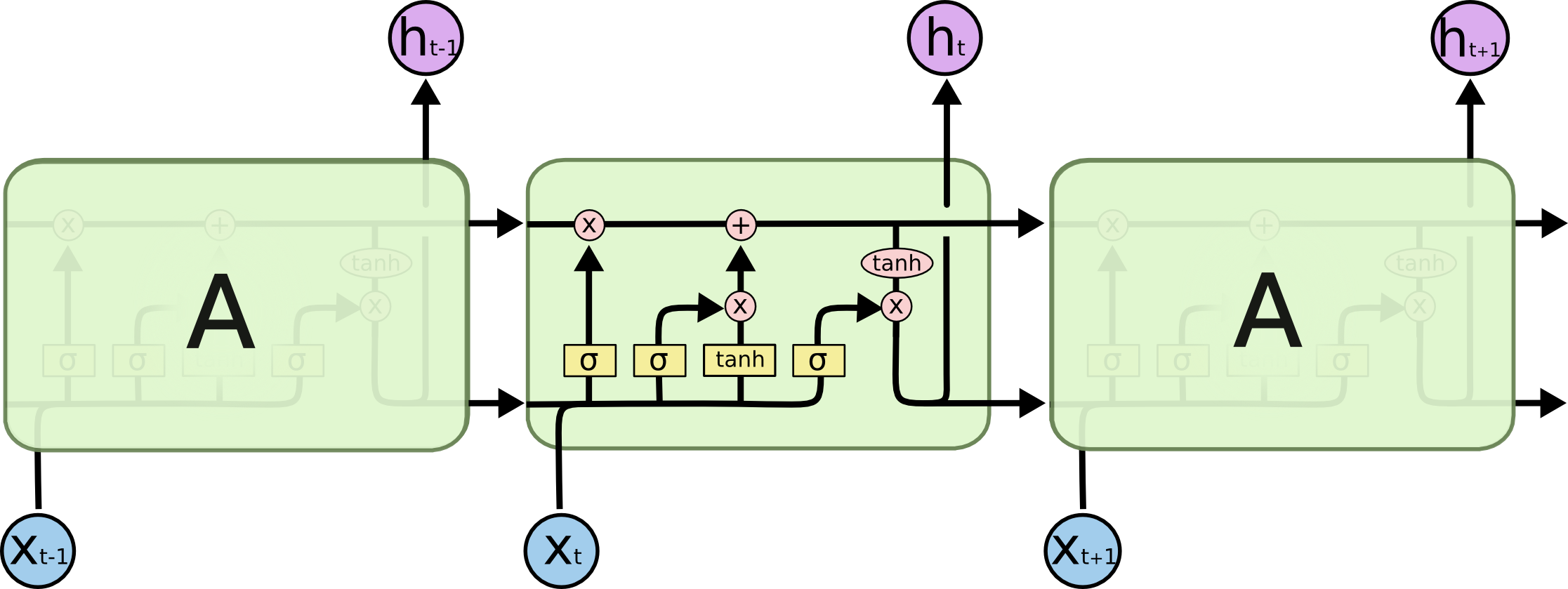
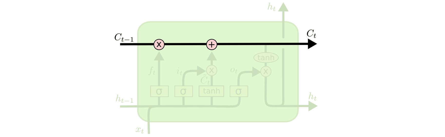
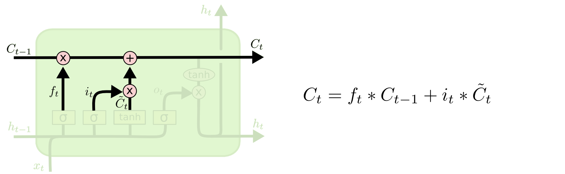
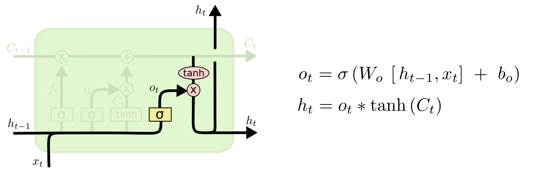
The Long Short-Term Memory (Hochreiter and Schmidhuber 1997) adds a cell state \(\mathbf{c}_t \in \mathbb{R}^H\) alongside the hidden state \(\mathbf{h}_t\).

Conceptual roles:

Variable Role Analogy
\(\mathbf{c}_t\) Long-term memory A conveyor belt running along the sequence
\(\mathbf{h}_t\) Short-term / output representation What you say aloud at each step
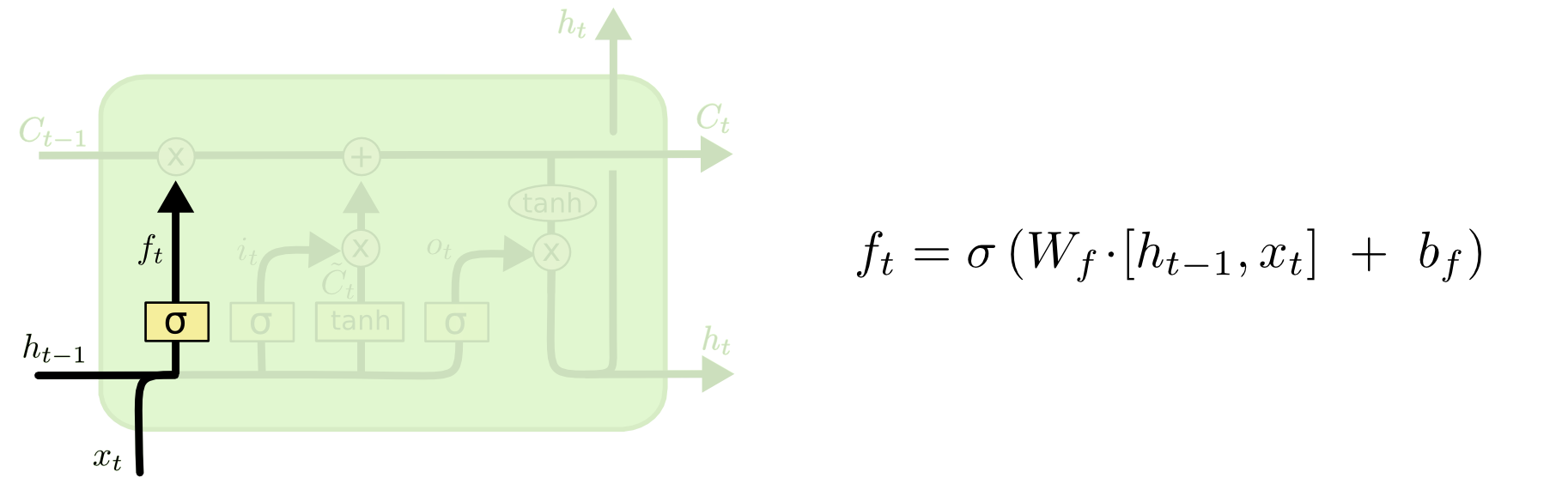
\(\mathbf{f}_t\) Forget gate How much of the old belt to erase
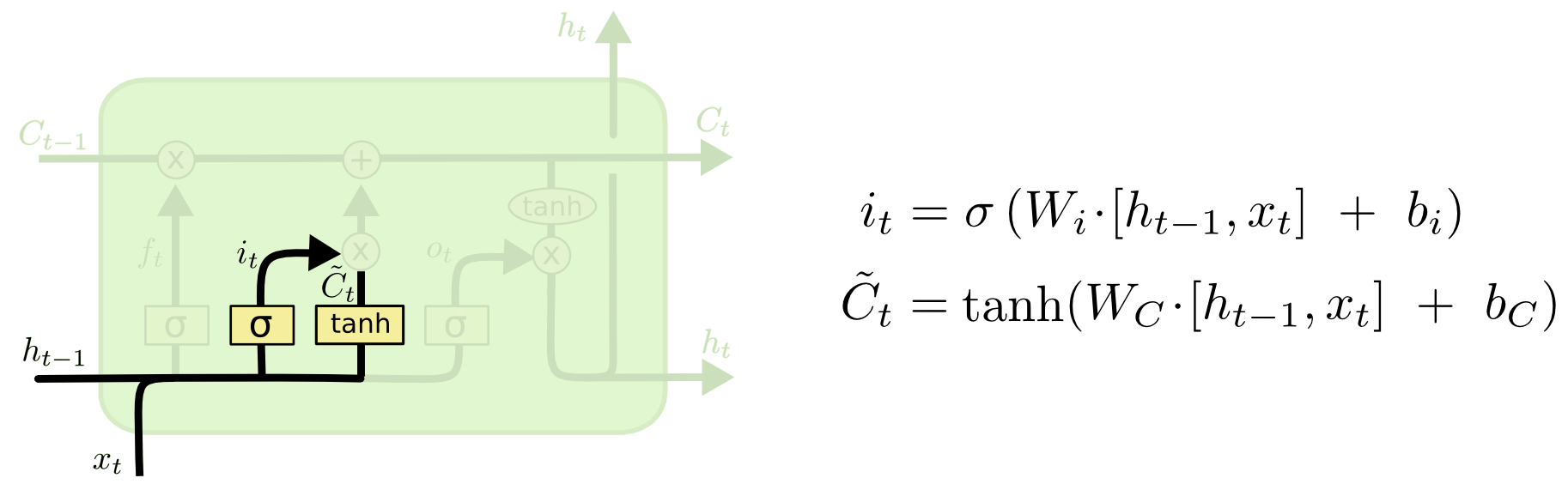
\(\mathbf{i}_t\) Input gate How much new info to write onto the belt
\(\mathbf{o}_t\) Output gate How much of the belt to “read” for \(\mathbf{h}_t\)

All gates produce values in \((0, 1)\) via sigmoid \(\sigma\); \(\mathbf{f}_t \approx 0\) means “erase”, \(\approx 1\) means “keep”.

LSTM gates

Let \([\mathbf{h}_{t-1}; \mathbf{x}_t] \in \mathbb{R}^{H+d}\) denote the concatenation of the previous hidden state and current input.

1. forget gate

\[ \mathbf{f}_t = \sigma\!\left(W_f\,[\mathbf{h}_{t-1};\mathbf{x}_t] + \mathbf{b}_f\right) \]

2. input gate

\[ \mathbf{i}_t = \sigma\!\left(W_i\,[\mathbf{h}_{t-1};\mathbf{x}_t] + \mathbf{b}_i\right) \]

3. candidate cell \[ \tilde{\mathbf{c}}_t = \tanh\!\left(W_c\,[\mathbf{h}_{t-1};\mathbf{x}_t] + \mathbf{b}_c\right) \]

cell update \[ \mathbf{c}_t = \mathbf{f}_t \odot \mathbf{c}_{t-1} \;+\; \mathbf{i}_t \odot \tilde{\mathbf{c}}_t \]

4. output gate \[ \mathbf{o}_t = \sigma\!\left(W_o\,[\mathbf{h}_{t-1};\mathbf{x}_t] + \mathbf{b}_o\right) \]

hidden state \[ \mathbf{h}_t = \mathbf{o}_t \odot \tanh(\mathbf{c}_t) \]

  • \(\odot\) denotes element-wise (Hadamard) product.
  • All weight matrices \(W_{\{f,i,c,o\}}\) have shape \((H, H+d)\); biases \(\mathbf{b}\) have shape \((H,)\).
  • Parameter count: \(4H(H + d) + 4H\) — four times a vanilla RNN.

Why the cell state is a gradient highway

The cell update is additive in \(\mathbf{c}_{t-1}\):

\[ \mathbf{c}_t = \underbrace{\mathbf{f}_t \odot \mathbf{c}_{t-1}}_{\text{old memory scaled}} + \underbrace{\mathbf{i}_t \odot \tilde{\mathbf{c}}_t}_{\text{new write}} \]

Taking the partial derivative of \(\mathbf{c}_t\) w.r.t. \(\mathbf{c}_{t-1}\):

\[ \frac{\partial \mathbf{c}_t}{\partial \mathbf{c}_{t-1}} = \operatorname{diag}(\mathbf{f}_t) \]

This is a diagonal matrix. When \(\mathbf{f}_t \approx \mathbf{1}\) (forget gate open), the gradient flows back through \(c\) with roughly no shrinkage.
Compare to vanilla RNN where the Jacobian is \(\operatorname{diag}(1 - \mathbf{h}_{t-1}^2) \cdot W_{hh}\) — a full matrix multiply at each step.

Takeaway

The cell state provides a near-identity gradient path when the forget gate is near 1.
The model learns when to open or close this path — it is not hardcoded.

🔬 Gradient flow — formal sketch

For a loss \(\mathcal{L}\) at the final step \(T\), the gradient w.r.t. cell state at time \(t\) is:

\[ \frac{\partial \mathcal{L}}{\partial \mathbf{c}_t} = \frac{\partial \mathcal{L}}{\partial \mathbf{c}_T} \cdot \prod_{k=t+1}^{T} \operatorname{diag}(\mathbf{f}_k) \]

Because each factor is diagonal and elementwise-bounded by \([0, 1]\):

  • When \(f_k^{(j)} \approx 1\) for all \(k\): the \(j\)-th gradient component survives all \(T - t\) steps undiluted.
  • When \(f_k^{(j)} \approx 0\) for some \(k\): the \(j\)-th gradient is intentionally killed — the network decided this memory slot is irrelevant beyond step \(k\).

Contrast with vanilla RNN:

\[ \frac{\partial \mathcal{L}}{\partial \mathbf{h}_t} = \frac{\partial \mathcal{L}}{\partial \mathbf{h}_T} \cdot \prod_{k=t+1}^{T} \left[\operatorname{diag}(1 - \mathbf{h}_k^2) \cdot W_{hh}\right] \]

Each factor is a full matrix, and powers of matrices with spectral radius \(< 1\) shrink exponentially.

The structural difference

LSTM replaces full-matrix products (multiplicative, potentially shrinking) with element-wise products (controllable, potentially identity-like). This is the core of why LSTMs can learn dependencies across hundreds of steps while vanilla RNNs cannot.

GRU: two gates, no separate cell state

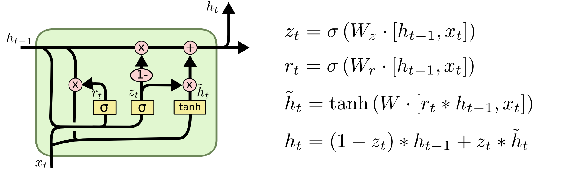
The Gated Recurrent Unit (Cho et al. 2014) simplifies the LSTM by merging the cell state and hidden state into one, with two gates:

\[ \begin{aligned} \mathbf{r}_t &= \sigma\!\left(W_r\,[\mathbf{h}_{t-1};\mathbf{x}_t] + \mathbf{b}_r\right) & \text{(reset gate)}\\ \mathbf{z}_t &= \sigma\!\left(W_z\,[\mathbf{h}_{t-1};\mathbf{x}_t] + \mathbf{b}_z\right) & \text{(update gate)}\\ \tilde{\mathbf{h}}_t &= \tanh\!\left(W_h\,[\mathbf{r}_t \odot \mathbf{h}_{t-1};\mathbf{x}_t] + \mathbf{b}_h\right) & \text{(candidate hidden)}\\ \mathbf{h}_t &= (1 - \mathbf{z}_t) \odot \mathbf{h}_{t-1} \;+\; \mathbf{z}_t \odot \tilde{\mathbf{h}}_t & \text{(hidden update)} \end{aligned} \]

Gate roles:

  • Reset gate \(\mathbf{r}_t\): how much of the past hidden state the candidate should see. \(\mathbf{r}_t \approx 0\) forces \(\tilde{\mathbf{h}}_t\) to ignore the past.
  • Update gate \(\mathbf{z}_t\): interpolation coefficient between old hidden state and new candidate. \(\mathbf{z}_t \approx 0\) → “carry old”; \(\mathbf{z}_t \approx 1\) → “write new”.

Parameter count: \(3H(H + d) + 3H\) — 75 % of LSTM.

LSTM vs GRU vs vanilla RNN: at a glance

Vanilla RNN GRU LSTM
Memory variables \(\mathbf{h}_t\) \(\mathbf{h}_t\) \(\mathbf{h}_t\), \(\mathbf{c}_t\)
Gates none 2 (reset, update) 3 (forget, input, output)
Params per layer \(H(H+d)+H\) \(3H(H+d)+3H\) \(4H(H+d)+4H\)
Long-range gradient ✗ (vanishes) ✓ (update gate) ✓ (cell highway)
Typical preference Short sequences Speed/efficiency Long sequences, tasks needing fine-grained control

Rule of thumb

Start with LSTM. If training time matters and sequences are not extremely long, try GRU. Vanilla RNNs are mainly used for pedagogical or very constrained settings today.

❌ Anti-example: using LSTM when vanilla RNN would suffice

Scenario:

  • Task: classify 3-word product titles as “electronics” or “clothing”.
  • Sequences are short; no long-range dependency exists.
  • A student reaches for nn.LSTM by default and reports slightly worse validation accuracy than a nn.RNN trained for the same number of steps.

Issues:

  1. Unnecessary complexity: LSTM has \(4\times\) the parameters of a vanilla RNN for the same hidden size. With very little data and short sequences, this extra capacity increases overfitting risk.
  2. Slower convergence: More parameters → more gradient updates needed before the gates settle into useful configurations.
  3. Misdiagnosis: The student suspects “LSTMs are worse” and may over-generalise. In reality, LSTMs are solving a problem (long-range gradients) that simply does not exist here.

Takeaway:

Match the architectural complexity to the task. The key question is always: how far back in the sequence does the relevant context actually reach?
For sequences of length ≤ 10–15, a well-regularized vanilla RNN or even a simple bag-of-words approach is often competitive.

Worked example 1

Long-range memory: T = 100

In M48 we showed a vanilla RNN can retrieve a seed value from 30 steps ago.
Now we push to T = 100 steps.

Task:

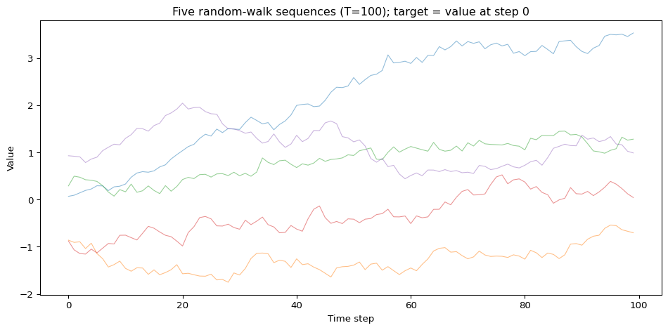
  • Input: a random walk \(x_0, x_1, \ldots, x_{T-1}\) of length \(T = 100\).
  • Target: predict the seed value \(x_0\) from the final hidden state.

Why this is a clean test:

  • There is exactly one relevant timestep: step 0.
  • A model that generalises must carry \(x_0\) in its state for 100 steps without corrupting it.
  • The theoretical noise floor (for an MLP or any model that can’t see step 0) is \(\text{Var}(x_0) \approx 0.083\).

We compare three models with the same hidden size (\(H = 32\)): vanilla RNN, LSTM, GRU.

Generate data

Code
import numpy as np
import pandas as pd
import matplotlib.pyplot as plt
import torch
import torch.nn as nn
from torch.utils.data import TensorDataset, DataLoader

rng = np.random.default_rng(3151)

T_SEQ = 100
N_TRAIN = 3000
N_VAL   = 500
SIGMA   = 0.1

def make_walk_data(n, T, sigma, rng):
    x0    = rng.uniform(-1, 1, size=(n,)).astype(np.float32)
    noise = rng.normal(0, sigma, size=(n, T)).astype(np.float32)
    seqs  = np.zeros((n, T), dtype=np.float32)
    seqs[:, 0] = x0
    for t in range(1, T):
        seqs[:, t] = seqs[:, t-1] + noise[:, t]
    # sequences shape: (n, T, 1), targets shape: (n,)
    return seqs[:, :, np.newaxis], x0

X_train, y_train = make_walk_data(N_TRAIN, T_SEQ, SIGMA, rng)
X_val,   y_val   = make_walk_data(N_VAL,   T_SEQ, SIGMA, rng)

print(f"X_train shape: {X_train.shape}, y_train shape: {y_train.shape}")

# Quick sanity plot
fig, ax = plt.subplots()
for i in range(5):
    ax.plot(X_train[i, :, 0], alpha=0.5, linewidth=0.8)
ax.set_xlabel("Time step")
ax.set_ylabel("Value")
ax.set_title("Five random-walk sequences (T=100); target = value at step 0")
plt.tight_layout()
X_train shape: (3000, 100, 1), y_train shape: (3000,)

Define and train the three models

Code
device = "cuda" if torch.cuda.is_available() else "cpu"

def make_loaders(X, y, X_v, y_v, bs=128):
    Xt = torch.from_numpy(X);  yt = torch.from_numpy(y)
    Xv = torch.from_numpy(X_v); yv = torch.from_numpy(y_v)
    return (DataLoader(TensorDataset(Xt, yt), batch_size=bs, shuffle=True),
            DataLoader(TensorDataset(Xv, yv), batch_size=256))

train_loader, val_loader = make_loaders(X_train, y_train, X_val, y_val)

H = 32

class SeqModel(nn.Module):
    def __init__(self, rnn_type="rnn", hidden=32):
        super().__init__()
        cls = {"rnn": nn.RNN, "lstm": nn.LSTM, "gru": nn.GRU}[rnn_type]
        self.rnn = cls(input_size=1, hidden_size=hidden, batch_first=True)
        self.head = nn.Linear(hidden, 1)
        self.rnn_type = rnn_type
    def forward(self, x):
        out, _ = self.rnn(x)
        last    = out[:, -1, :]   # hidden state at step T-1
        return self.head(last).squeeze(-1)

def count_params(m):
    return sum(p.numel() for p in m.parameters())

models = {name: SeqModel(name, H).to(device) for name in ["rnn", "lstm", "gru"]}
for name, m in models.items():
    print(f"{name.upper():4s}: {count_params(m):,} params")
RNN : 1,153 params
LSTM: 4,513 params
GRU : 3,393 params

Training loop

Code
def train_model(model, tl, vl, epochs=60, lr=3e-3):      # TODO epochs -> 120
    opt  = torch.optim.Adam(model.parameters(), lr=lr)
    loss_fn = nn.MSELoss()
    hist = {"epoch": [], "train_mse": [], "val_mse": []}
    for ep in range(1, epochs + 1):
        model.train()
        t_loss, t_n = 0.0, 0
        for xb, yb in tl:
            xb, yb = xb.to(device), yb.to(device)
            opt.zero_grad()
            pred = model(xb)
            loss = loss_fn(pred, yb)
            loss.backward()
            torch.nn.utils.clip_grad_norm_(model.parameters(), 5.0)
            opt.step()
            t_loss += loss.item() * xb.size(0); t_n += xb.size(0)
        model.eval()
        v_loss, v_n = 0.0, 0
        with torch.no_grad():
            for xb, yb in vl:
                xb, yb = xb.to(device), yb.to(device)
                v_loss += loss_fn(model(xb), yb).item() * xb.size(0); v_n += xb.size(0)
        hist["epoch"].append(ep)
        hist["train_mse"].append(t_loss / t_n)
        hist["val_mse"].append(v_loss / v_n)
    return pd.DataFrame(hist)

histories = {name: train_model(m, train_loader, val_loader) for name, m in models.items()}

Learning curves: T=100

Code
naive_floor = float(np.var(y_train))
noise_floor = SIGMA**2

fig, ax = plt.subplots(figsize=(9, 4))
colours = {"rnn": "steelblue", "lstm": "darkorange", "gru": "forestgreen"}
for name, hist in histories.items():
    ax.plot(hist["epoch"], hist["val_mse"],
            label=f"{name.upper()} val", color=colours[name])
    ax.plot(hist["epoch"], hist["train_mse"],
            linestyle="--", alpha=0.4, color=colours[name])

ax.axhline(naive_floor, color="red",    linestyle=":", linewidth=1.5,
           label=f"Naive floor Var(x₀)={naive_floor:.3f}")
ax.axhline(noise_floor, color="purple", linestyle=":", linewidth=1.5,
           label=f"Noise floor σ²={noise_floor:.3f}")
ax.set_yscale("log")
ax.set_xlabel("Epoch"); ax.set_ylabel("MSE (log scale)")
ax.set_title("Long-range memory retrieval at T=100")
ax.legend(fontsize=8)
plt.tight_layout()

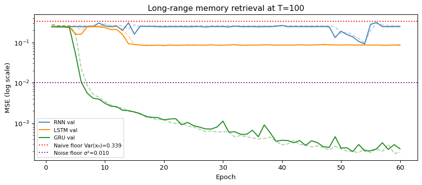
All three models vs the naive floor (Var(x₀) ≈ 0.083) and noise floor (σ²=0.01).

Summary table

Code
rows = []
for name, hist in histories.items():
    rows.append({
        "Model":         name.upper(),
        "Params":        f"{count_params(models[name]):,}",
        "Final val MSE": round(hist["val_mse"].iloc[-1], 5),
        "Beats naive floor?": "✓" if hist["val_mse"].iloc[-1] < naive_floor else "✗",
        "Approaches noise floor?": "✓" if hist["val_mse"].iloc[-1] < 5 * noise_floor else "✗",
    })
pd.DataFrame(rows)
Model Params Final val MSE Beats naive floor? Approaches noise floor?
0 RNN 1,153 0.24676
1 LSTM 4,513 0.08639
2 GRU 3,393 0.00023

Key observation:

At T=100, the vanilla RNN typically fails to cross the naive floor — it cannot reliably remember \(x_0\).
Both LSTM and GRU cross it and approach the noise floor, demonstrating that gated architectures can carry information across 100 steps while vanilla RNNs cannot.

Worked example 2

Sentiment classification: SST-2 subset

We use a 2 000-example subset of the 🔗 Stanford Sentiment Treebank (SST-2):

  • Binary task: classify a movie review snippet as 👍positive or 👎negative.
  • Average review length: ~20 tokens — moderate, not trivially short.
  • Vocabulary: top 5 000 words; fixed 30-token padded sequences.

Why this task?

  • Sentiment often depends on negation and context that spans several words: “not at all bad” — the word “not” needs to influence the interpretation of “bad” 3 steps later.
  • Long-range dependencies are real but not extreme, making this a good intermediate test.

Goal: compare vanilla RNN, LSTM, and GRU on accuracy and training stability.

Load and preprocess SST-2 (subset)

Code
from collections import Counter
import re
from datasets import load_dataset
import random


# ── Real SST-2 subsample (5 000 train + 400 validation) ───────────────────────
# Loads from HuggingFace Hub; requires network access.
# The official SST-2 validation split has no labels publicly, so we carve our
# own val set from the training split.

N_SAMPLES  = 5000
VAL_FRAC   = 0.2
MAX_LEN    = 30
VOCAB_SIZE = 5000
EMBED_DIM  = 64

random.seed(3151)
np.random.seed(3151)
torch.manual_seed(3151)
torch.cuda.manual_seed_all(3151)
torch.backends.cudnn.deterministic = True
torch.backends.cudnn.benchmark     = False

raw = (load_dataset("stanfordnlp/sst2", split="train")
       .shuffle(seed=3151)
       .select(range(N_SAMPLES)))

# ── Build a simple word-level vocabulary from this subsample ──────────────────
def tokenize(text):
    return re.findall(r"[a-z]+", text.lower())

all_tokens = [tok for ex in raw for tok in tokenize(ex["sentence"])]
vocab_counts = Counter(all_tokens)
# token→index: 0=PAD, 1=UNK, then top (VOCAB_SIZE-2) words
idx2tok = ["<PAD>", "<UNK>"] + [w for w, _ in vocab_counts.most_common(VOCAB_SIZE - 2)]
tok2idx = {w: i for i, w in enumerate(idx2tok)}

def encode(text, max_len=MAX_LEN):
    ids = [tok2idx.get(t, 1) for t in tokenize(text)][:max_len]
    ids += [0] * (max_len - len(ids))          # right-pad with PAD=0
    return ids

X_sst = np.array([encode(ex["sentence"]) for ex in raw], dtype=np.int64)
y_sst = np.array([ex["label"]            for ex in raw], dtype=np.int64)

split = int((1 - VAL_FRAC) * N_SAMPLES)
Xtr_s, Xvl_s = X_sst[:split], X_sst[split:]
ytr_s, yvl_s = y_sst[:split], y_sst[split:]

g = torch.Generator()
g.manual_seed(3151)

sst_train_loader = DataLoader(
    TensorDataset(torch.from_numpy(Xtr_s), torch.from_numpy(ytr_s)),
    batch_size=64, shuffle=True, generator=g)
sst_val_loader = DataLoader(
    TensorDataset(torch.from_numpy(Xvl_s), torch.from_numpy(yvl_s)),
    batch_size=256)

print(f"Train: {Xtr_s.shape}  Val: {Xvl_s.shape}")
print(f"Class balance — train: {np.bincount(ytr_s)}, val: {np.bincount(yvl_s)}")
print(f"Vocab size used: {len(tok2idx)}")
Train: (4000, 30)  Val: (1000, 30)
Class balance — train: [1755 2245], val: [440 560]
Vocab size used: 5000

Sentiment model: embed → recurrent → classify

Code
class SentimentModel(nn.Module):
    def __init__(self, rnn_type="lstm", vocab=VOCAB_SIZE,
                 embed_dim=EMBED_DIM, hidden=64, num_classes=2):
        super().__init__()
        self.embed = nn.Embedding(vocab, embed_dim, padding_idx=0)
        cls = {"rnn": nn.RNN, "lstm": nn.LSTM, "gru": nn.GRU}[rnn_type]
        self.rnn  = cls(embed_dim, hidden, batch_first=True)
        self.drop = nn.Dropout(0.3)
        self.head = nn.Linear(hidden, num_classes)
        self.rnn_type = rnn_type

    def forward(self, x):
        emb  = self.drop(self.embed(x))        # (B, T, E)
        out, _ = self.rnn(emb)
        last = out[:, -1, :]                   # last hidden state
        return self.head(self.drop(last))

sst_models = {n: SentimentModel(n).to(device) for n in ["rnn", "lstm", "gru"]}
for n, m in sst_models.items():
    print(f"{n.upper():4s}: {count_params(m):,} params")
RNN : 328,450 params
LSTM: 353,410 params
GRU : 345,090 params

Train & evaluate

Code
def train_classifier(model, tl, vl, epochs=10, lr=1e-3, patience=7):
    opt     = torch.optim.Adam(model.parameters(), lr=lr)
    loss_fn = nn.CrossEntropyLoss()
    hist = {"epoch": [], "train_acc": [], "val_acc": [], "val_loss": []}

    best_val_loss = float("inf")
    epochs_no_improve = 0
    for ep in range(1, epochs + 1):
        model.train()
        t_correct, t_n = 0, 0
        for xb, yb in tl:
            xb, yb = xb.to(device), yb.to(device)
            opt.zero_grad()
            logits = model(xb)
            loss   = loss_fn(logits, yb)
            loss.backward()
            torch.nn.utils.clip_grad_norm_(model.parameters(), 5.0)
            opt.step()
            t_correct += (logits.argmax(1) == yb).sum().item(); t_n += yb.size(0)

        model.eval()
        v_correct, v_n, v_loss_sum = 0, 0, 0.0
        with torch.no_grad():
            for xb, yb in vl:
                xb, yb = xb.to(device), yb.to(device)
                logits = model(xb)
                v_loss_sum += loss_fn(logits, yb).item() * yb.size(0)
                v_correct  += (logits.argmax(1) == yb).sum().item(); v_n += yb.size(0)

        if v_loss_sum / v_n < best_val_loss:
            best_val_loss = v_loss_sum / v_n
            epochs_no_improve = 0
        else:
            epochs_no_improve += 1
            if epochs_no_improve >= patience:
                break

        hist["epoch"].append(ep)
        hist["train_acc"].append(t_correct / t_n)
        hist["val_acc"].append(v_correct / v_n)
        hist["val_loss"].append(v_loss_sum / v_n)

    return pd.DataFrame(hist)

sst_hists = {n: train_classifier(m, sst_train_loader, sst_val_loader)
             for n, m in sst_models.items()}

Accuracy curves: sentiment

Code
fig, axes = plt.subplots(1, 2, figsize=(11, 4))

for name, hist in sst_hists.items():
    axes[0].plot(hist["epoch"], hist["val_acc"],   label=f"{name.upper()} val",   color=colours[name])
    axes[0].plot(hist["epoch"], hist["train_acc"], linestyle="--", alpha=0.35,    color=colours[name])
    axes[1].plot(hist["epoch"], hist["val_loss"],  label=f"{name.upper()} val loss", color=colours[name])

axes[0].axhline(0.5, color="gray", linestyle=":", label="Chance")
axes[0].set_xlabel("Epoch"); axes[0].set_ylabel("Accuracy")
axes[0].set_title("Accuracy (solid=val, dashed=train)"); axes[0].legend(fontsize=8)

axes[1].set_xlabel("Epoch"); axes[1].set_ylabel("Cross-entropy loss")
axes[1].set_title("Validation loss"); axes[1].legend(fontsize=8)

plt.tight_layout()

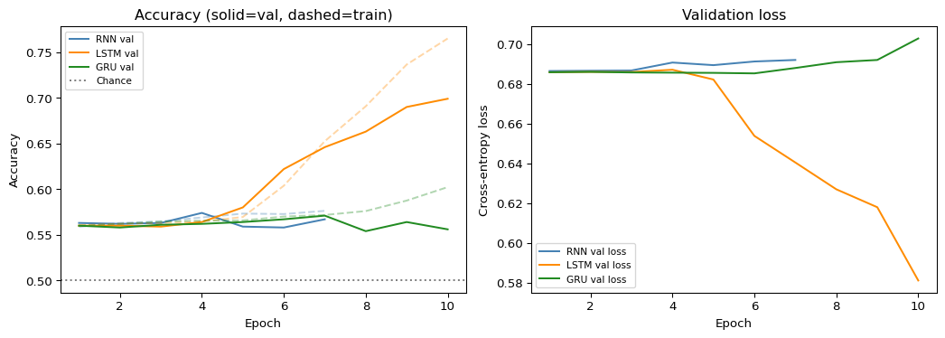
Validation accuracy over 20 epochs for RNN, LSTM, and GRU on SST-2 subset.

Comparison table: sentiment

Code
rows2 = []
for name, hist in sst_hists.items():
    best_val = hist["val_acc"].max()
    final_gap = hist["train_acc"].iloc[-1] - hist["val_acc"].iloc[-1]
    rows2.append({
        "Model":           name.upper(),
        "Params":          f"{count_params(sst_models[name]):,}",
        "Best val acc":    round(best_val, 3),
        "Train–val gap":   round(final_gap, 3),
    })
pd.DataFrame(rows2)
Model Params Best val acc Train–val gap
0 RNN 328,450 0.574 0.009
1 LSTM 353,410 0.699 0.066
2 GRU 345,090 0.571 0.046

Design choice to notice

For sequences of moderate length (~30 tokens), LSTM and GRU often outperform the vanilla RNN — but the gap shrinks as sequences get shorter. Always compare empirically rather than assuming “LSTM is always better.”
The train–val gap is a useful proxy for how much the model is overfitting given the small dataset.

Summary

Choosing your recurrent cell

Situation Recommendation Reason
Short sequences (< 15 tokens) Vanilla RNN or even bag-of-words No long-range dependency; extra gates add cost without benefit
Moderate sequences (15–100) GRU first Fewer params than LSTM, fast to train, competitive accuracy
Long sequences (100+) or tasks requiring fine-grained memory control LSTM Cell state highway helps; output gate decouples memory from representation
Compute-constrained / mobile GRU 75 % of LSTM params; often matches performance
Cutting-edge NLP (2024+) Transformer Attention has replaced recurrence for most large-scale tasks

Quick diagnostic

  1. Does your validation loss plateau while training loss keeps falling? → likely overfitting; reduce capacity or add dropout.
  2. Do both losses plateau early at a high value? → likely underfitting; increase hidden size or train longer.
  3. Does LSTM outperform GRU substantially? → the task probably requires fine-grained cell control.

Ethics & risks in gated sequence models

1. Long-range context amplifies biased associations:

  • LSTM/GRU can remember and condition on early context for hundreds of steps.
  • If the training corpus encodes stereotypes (e.g., gender–profession correlations in text), gated models can leverage that context more persistently than a vanilla RNN would.
  • Example: a sentiment model trained on review text may associate certain names or dialects with positive or negative sentiment and carry that context across the full review.

2. Memorisation of sensitive sequences:

  • Long hidden states in LSTMs trained on personal data (medical notes, chat logs, location traces) can encode individual-specific patterns.
  • These can be extracted via model inversion or membership-inference attacks.
  • Mitigation: differential privacy training (e.g., DP-SGD), careful data minimisation, and evaluation for memorisation before deployment.

3. Opaque temporal reasoning:

  • Unlike a bag-of-words model, a gated RNN’s decision is influenced by a hidden state that is hard to inspect.
  • When deployed in high-stakes settings (medical, legal, financial), temporal models should be paired with interpretability tools (attention visualization, SHAP for time series, or integrated gradients).

Simple check: Before deploying a gated RNN, ask: What information from the past could the model be weighting heavily? Could that information encode protected attributes or be used to discriminate?

Quick checks

Q1. An LSTM has input size \(d = 10\), hidden size \(H = 20\).

How many trainable parameters does this LSTM have (excluding any output head)?

  1. \(20 \times (10 + 20) + 20 = 620\)

  2. \(4 \times [20 \times (10 + 20) + 20] = 2480\)

  3. \(4 \times [20 \times 10 + 20] = 960\)

  4. \(3 \times [20 \times (10 + 20) + 20] = 1860\)

Q2. Short answer: In the LSTM cell update \(\mathbf{c}_t = \mathbf{f}_t \odot \mathbf{c}_{t-1} + \mathbf{i}_t \odot \tilde{\mathbf{c}}_t\), what happens when the forget gate \(\mathbf{f}_t \approx \mathbf{0}\) and the input gate \(\mathbf{i}_t \approx \mathbf{1}\)? Describe the effect on memory and identify a natural use case.

Model answer: The cell state is almost entirely replaced by the new candidate \(\tilde{\mathbf{c}}_t\). This is a “hard reset” — the old long-term memory is erased and rewritten with the current input. A natural use case: the beginning of a new sentence or document in a streaming text task, where the previous context is irrelevant and the model should start fresh.

Q3. In the GRU, the candidate hidden state is computed as \(\tilde{\mathbf{h}}_t = \tanh(W_h[\mathbf{r}_t \odot \mathbf{h}_{t-1};\, \mathbf{x}_t] + \mathbf{b}_h)\).

What does setting the reset gate \(\mathbf{r}_t \approx \mathbf{0}\) effectively do?

  1. Forces the GRU to fully copy the old hidden state \(\mathbf{h}_{t-1}\) to \(\mathbf{h}_t\).

  2. Makes the candidate \(\tilde{\mathbf{h}}_t\) ignore \(\mathbf{h}_{t-1}\), so the update depends only on \(\mathbf{x}_t\).

  3. Sets \(\mathbf{h}_t \approx \mathbf{h}_{t-1}\) regardless of \(\mathbf{x}_t\).

  4. Doubles the effective learning rate for this time step.

Q4. Numeric / reasoning: Consider a sequence classification task where the relevant label signal is contained only in the last 3 tokens of a length-50 sequence (e.g., “…, nothing, wrong, here → positive”).

A student trains a vanilla RNN for 200 epochs and a GRU for 100 epochs (same hidden size, same data). The GRU converges faster to higher validation accuracy.

Provide one architectural explanation for the GRU’s advantage, and one training-setup reason that might make the comparison unfair.

References

Cho, Kyunghyun, Bart van Merriënboer, Caglar Gulcehre, Dzmitry Bahdanau, Fethi Bougares, Holger Schwenk, and Yoshua Bengio. 2014. “Learning Phrase Representations Using RNN Encoder–Decoder for Statistical Machine Translation.” In Proceedings of the 2014 Conference on Empirical Methods in Natural Language Processing (EMNLP), 1724–34. Association for Computational Linguistics. https://doi.org/10.3115/v1/D14-1179.
Hochreiter, Sepp, and Jürgen Schmidhuber. 1997. “Long Short-Term Memory.” Neural Computation 9 (8): 1735–80. https://doi.org/10.1162/neco.1997.9.8.1735.