CSCI 3151 — Foundations of Machine Learning
By the end of this module, you should be able to:
A sequence is an ordered collection of items where position/order matters.
| Domain | Input sequence | Output |
|---|---|---|
| Language | Words in a sentence | Next word / sentiment |
| Audio | Frames of a speech signal | Phoneme / transcription |
| Time series | Daily temperature readings | Tomorrow’s forecast |
| Biology | Nucleotides in a genome | Protein function |
| Finance | Closing prices over days | Future price / anomaly |
Key difference from tabular data:
Id Est
A sequence model must use the history of what it has seen to produce a sensible output at each step.
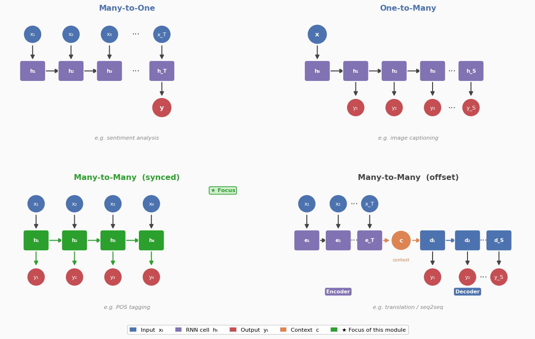
Different tasks impose different input/output structures:

We’ll mostly focus on many-to-one and many-to-many (synced).
Scenario: You have sentences of up to 50 words and want to classify sentiment.
Naïve approach: Concatenate all word vectors into one big vector → pass to an MLP.
Problems:
Takeaway:
A feedforward net has no memory and no positional invariance. Sequences need architectures that are designed around temporal order and shared parameters across time.
A recurrent neural network (RNN) maintains a hidden state \(\mathbf{h}_t\) that is updated at each time step \(t\):
\[ \mathbf{h}_t = f\!\left(W_{hh}\,\mathbf{h}_{t-1} + W_{xh}\,\mathbf{x}_t + \mathbf{b}_h\right) \]
\[ \mathbf{y}_t = W_{hy}\,\mathbf{h}_t + \mathbf{b}_y \]
Variables:
| Symbol | Shape | Meaning |
|---|---|---|
| \(\mathbf{x}_t\) | \((d,)\) | Input at step \(t\) |
| \(\mathbf{h}_t\) | \((H,)\) | Hidden state at step \(t\) |
| \(W_{xh}\) | \((H, d)\) | Input-to-hidden weights |
| \(W_{hh}\) | \((H, H)\) | Hidden-to-hidden weights |
| \(W_{hy}\) | \((K, H)\) | Hidden-to-output weights |
| \(f\) | — | Element-wise nonlinearity (e.g., \(\tanh\)) |
Critical property: \(W_{hh}\), \(W_{xh}\), \(W_{hy}\) are shared across all time steps. One set of weights, many steps.
We can visualise the RNN “unrolled” through time — this makes it look like a very deep feedforward network:
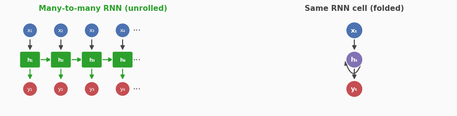
Each [h_t] box applies the same weights \((W_{xh}, W_{hh}, W_{hy})\).
Key analogy:
Unrolling in time ↔︎ a very deep network in depth.
The depth equals the sequence length \(T\).
For \(T = 100\), you effectively have a 100-layer network with tied weights.
This is exactly why gradient problems (M33–M34) arise here too — but we’ll get there.
Initial state \(\mathbf{h}_0\): Often set to the zero vector. Sometimes learned.
The same weight matrix \(W_{hh}\) appears at every step.
Benefits:
Contrast with CNNs (from M44):
| Property | CNN | RNN |
|---|---|---|
| Shared weights | Over spatial positions | Over time steps |
| Inductive bias | Local spatial patterns | Temporal order & history |
| “Memory” | Receptive field | Hidden state \(\mathbf{h}_t\) |
Both share weights — just in different dimensions.
Let’s trace a tiny example by hand.
Setup: \(d = 2\), \(H = 2\), \(K = 1\) (scalar output). \(T = 3\) steps.
Suppose:
\[ W_{xh} = \begin{pmatrix} 0.5 & 0 \\ 0 & 0.5 \end{pmatrix}, \quad W_{hh} = \begin{pmatrix} 0.2 & 0 \\ 0 & 0.2 \end{pmatrix}, \quad \mathbf{b}_h = \mathbf{0} \]
\[ \mathbf{x}_1 = (1, 0)^\top, \quad \mathbf{x}_2 = (0, 1)^\top, \quad \mathbf{x}_3 = (1, 1)^\top \]
\[ \mathbf{h}_0 = (0, 0)^\top \]
Step 1: \[\mathbf{h}_1 = \tanh(W_{hh}\mathbf{h}_0 + W_{xh}\mathbf{x}_1) = \tanh\!\begin{pmatrix}0.5\\0\end{pmatrix} = \begin{pmatrix}0.462\\0\end{pmatrix}\]
Step 2: \[\mathbf{h}_2 = \tanh\!\left(\begin{pmatrix}0.092\\0\end{pmatrix} + \begin{pmatrix}0\\0.5\end{pmatrix}\right) = \tanh\!\begin{pmatrix}0.092\\0.5\end{pmatrix} \approx \begin{pmatrix}0.092\\0.462\end{pmatrix}\]
Step 3: \(\mathbf{h}_3 = \tanh(W_{hh}\mathbf{h}_2 + W_{xh}\mathbf{x}_3) \approx \tanh\!\begin{pmatrix}0.518\\0.592\end{pmatrix} \approx \begin{pmatrix}0.479\\0.530\end{pmatrix}\)
Notice: \(\mathbf{h}_3\) encodes information from all three input steps.
Training an RNN = minimizing a loss over the whole sequence.
For many-to-one (e.g., sentiment):
\[\mathcal{L} = \ell\!\left(\hat{y}_T, y\right)\]
For many-to-many (e.g., time-series forecasting):
\[\mathcal{L} = \frac{1}{T} \sum_{t=1}^T \ell\!\left(\hat{y}_t, y_t\right)\]
BPTT is just standard backpropagation on the unrolled graph:
Key gradient equation (chain rule unrolled over time):
\[f \frac{\partial \mathcal{L}}{\partial \mathbf{h}_1} = \frac{\partial \mathbf{h}_T}{\partial \mathbf{h}_1} \cdot \frac{\partial \mathcal{L}}{\partial \mathbf{h}_T} = \left(\prod_{t=2}^{T} \frac{\partial \mathbf{h}_t}{\partial \mathbf{h}_{t-1}}\right) \cdot \frac{\partial \mathcal{L}}{\partial \mathbf{h}_T} \]
That product of Jacobians is exactly what causes vanishing/exploding gradients (recall M33–M34).
Each Jacobian factor is: \[ \frac{\partial \mathbf{h}_t}{\partial \mathbf{h}_{t-1}} = \text{diag}(f'(\cdot)) \cdot W_{hh} \]
where \(f' = 1 - \tanh^2(\cdot) \in (0, 1]\).
For \(T\) steps, the product has \(T-1\) such factors. The spectral radius of \(W_{hh}\) controls behaviour:
Truncated BPTT
In practice, gradients are only propagated \(k\) steps back (e.g., \(k = 20\)). This limits memory and stabilises training but means the model cannot learn dependencies longer than \(k\) steps.
This analysis directly motivates gated architectures (LSTMs, GRUs) in M49.
Motivation for the task design:
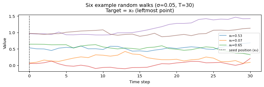
Task: Given a random walk sequence of length \(T = 30\), recover the starting value \(x_0\).
Why this is hard for an MLP
import numpy as np
import matplotlib.pyplot as plt
import pandas as pd
import torch
import torch.nn as nn
from torch.utils.data import TensorDataset, DataLoader
rng = np.random.default_rng(3151)
T_SEQ = 30 # full sequence length seen by the RNN
W_MLP = 5 # short window seen by the MLP
SIGMA = 0.05 # per-step noise std
N_TRAIN = 4000
N_VAL = 1000
def make_walks(n, T, sigma, rng):
"""Generate n random walks of length T+1 starting from U(0,1)."""
x0 = rng.uniform(0, 1, size=(n, 1)) # seed: (n, 1)
noise = rng.normal(0, sigma, size=(n, T)) # increments: (n, T)
steps = np.cumsum(noise, axis=1) # cumulative drift
walks = np.concatenate([x0, x0 + steps], axis=1) # (n, T+1)
return walks.astype(np.float32)
walks_train = make_walks(N_TRAIN, T_SEQ, SIGMA, rng)
walks_val = make_walks(N_VAL, T_SEQ, SIGMA, rng)
# Target: x_0 (the seed, first column)
y_train = walks_train[:, 0:1] # (N_TRAIN, 1)
y_val = walks_val[:, 0:1]
# RNN input: full walk x_0 … x_{T-1} (T steps) — shape (N, T, 1)
X_rnn_train = walks_train[:, :T_SEQ, np.newaxis]
X_rnn_val = walks_val[:, :T_SEQ, np.newaxis]
# MLP input: last W_MLP steps only — shape (N, W_MLP)
X_mlp_train = walks_train[:, -W_MLP:]
X_mlp_val = walks_val[:, -W_MLP:]
# Plot a few example walks
fig, ax = plt.subplots(figsize=(9, 3))
for i in range(6):
ax.plot(walks_train[i], alpha=0.6, label=f"x₀={walks_train[i,0]:.2f}" if i < 3 else None)
ax.axvline(x=0, color="k", linestyle=":", linewidth=1.5, label="seed position (x₀)")
ax.set_xlabel("Time step")
ax.set_ylabel("Value")
ax.set_title(f"Six example random walks (σ={SIGMA}, T={T_SEQ})\nTarget = x₀ (leftmost point)")
ax.legend(fontsize=8)
plt.tight_layout()
fig, axes = plt.subplots(1, 2, figsize=(10, 3.5))
example = walks_train[0]
ax = axes[0]
ax.plot(np.arange(T_SEQ + 1), example, marker="o", markersize=4)
ax.axvspan(T_SEQ - W_MLP, T_SEQ, alpha=0.2, color="orange", label=f"MLP window (last {W_MLP})")
ax.axvline(0, color="red", linestyle="--", label=f"x₀ = {example[0]:.2f} (target)")
ax.set_xlabel("Time step"); ax.set_ylabel("Value")
ax.set_title("One walk: what the MLP sees"); ax.legend(fontsize=8)
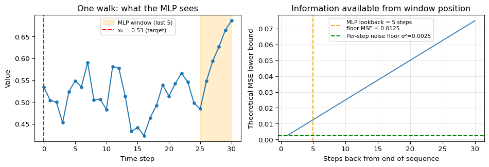
# Theoretical MSE floor for MLP: variance of (x_0 - x_{T-k}) = k * sigma^2
steps_back = np.arange(1, T_SEQ + 1)
theoretical_mse = steps_back * SIGMA**2
ax2 = axes[1]
ax2.plot(steps_back, theoretical_mse, color="steelblue")
ax2.axvline(W_MLP, color="orange", linestyle="--",
label=f"MLP lookback = {W_MLP} steps\nfloor MSE ≈ {W_MLP * SIGMA**2:.4f}")
ax2.axhline(SIGMA**2, color="green", linestyle="--",
label=f"Per-step noise floor σ²={SIGMA**2:.4f}")
ax2.set_xlabel("Steps back from end of sequence")
ax2.set_ylabel("Theoretical MSE lower bound")
ax2.set_title("Information available from window position")
ax2.legend(fontsize=8); ax2.grid(True, alpha=0.3)
plt.tight_layout()
device = "cuda" if torch.cuda.is_available() else "cpu"
# --- DataLoaders ---
def rnn_loader(X, y, batch_size=128, shuffle=True):
ds = TensorDataset(torch.from_numpy(X), torch.from_numpy(y))
return DataLoader(ds, batch_size=batch_size, shuffle=shuffle)
def mlp_loader(X, y, batch_size=128, shuffle=True):
ds = TensorDataset(torch.from_numpy(X), torch.from_numpy(y))
return DataLoader(ds, batch_size=batch_size, shuffle=shuffle)
rnn_train_loader = rnn_loader(X_rnn_train, y_train)
rnn_val_loader = rnn_loader(X_rnn_val, y_val, shuffle=False)
mlp_train_loader = mlp_loader(X_mlp_train, y_train)
mlp_val_loader = mlp_loader(X_mlp_val, y_val, shuffle=False)
# --- Models ---
class VanillaRNN(nn.Module):
"""RNN sees the full walk (T=30 steps) and outputs a prediction of x_0."""
def __init__(self, hidden_size=64):
super().__init__()
self.rnn = nn.RNN(1, hidden_size, batch_first=True, nonlinearity="tanh")
self.head = nn.Linear(hidden_size, 1)
def forward(self, x): # x: (B, T, 1)
out, _ = self.rnn(x)
return self.head(out[:, -1, :]) # use final hidden state
class MLPBaseline(nn.Module):
"""MLP sees only the last W_MLP steps; genuinely cannot see x_0."""
def __init__(self, window=W_MLP, hidden_size=64):
super().__init__()
self.net = nn.Sequential(
nn.Linear(window, hidden_size), nn.ReLU(),
nn.Linear(hidden_size, hidden_size), nn.ReLU(),
nn.Linear(hidden_size, 1)
)
def forward(self, x): # x: (B, W_MLP)
return self.net(x)
rnn_model = VanillaRNN(hidden_size=64).to(device)
mlp_model = MLPBaseline(hidden_size=64).to(device)
# Naive baseline: predict the mean of training seeds (≈ 0.5)
naive_val_mse = float(np.mean((y_val - y_train.mean())**2))
print(f"RNN params : {sum(p.numel() for p in rnn_model.parameters())}")
print(f"MLP params : {sum(p.numel() for p in mlp_model.parameters())}")
print(f"Naive (predict-mean) val MSE: {naive_val_mse:.4f} "
f"[theoretical MLP floor ≈ {W_MLP * SIGMA**2:.4f}]")RNN params : 4353
MLP params : 4609
Naive (predict-mean) val MSE: 0.0836 [theoretical MLP floor ≈ 0.0125]
def train_model(model, train_loader, val_loader, epochs=80, lr=1e-3):
model = model.to(device)
opt = torch.optim.Adam(model.parameters(), lr=lr)
loss_fn = nn.MSELoss()
history = {"epoch": [], "train_mse": [], "val_mse": []}
for epoch in range(1, epochs + 1):
model.train()
t_loss, t_n = 0.0, 0
for xb, yb in train_loader:
xb, yb = xb.to(device), yb.to(device)
opt.zero_grad()
loss = loss_fn(model(xb), yb)
loss.backward()
torch.nn.utils.clip_grad_norm_(model.parameters(), max_norm=5.0)
opt.step()
t_loss += loss.item() * xb.size(0); t_n += xb.size(0)
model.eval()
v_loss, v_n = 0.0, 0
with torch.no_grad():
for xb, yb in val_loader:
xb, yb = xb.to(device), yb.to(device)
v_loss += loss_fn(model(xb), yb).item() * xb.size(0); v_n += xb.size(0)
history["epoch"].append(epoch)
history["train_mse"].append(t_loss / t_n)
history["val_mse"].append(v_loss / v_n)
return pd.DataFrame(history)
hist_rnn = train_model(rnn_model, rnn_train_loader, rnn_val_loader, epochs=80)
hist_mlp = train_model(mlp_model, mlp_train_loader, mlp_val_loader, epochs=80)theoretical_floor = W_MLP * SIGMA**2
fig, ax = plt.subplots()
ax.plot(hist_rnn["epoch"], hist_rnn["train_mse"], label="RNN train")
ax.plot(hist_rnn["epoch"], hist_rnn["val_mse"], label="RNN val")
ax.plot(hist_mlp["epoch"], hist_mlp["train_mse"], label="MLP train", linestyle="--")
ax.plot(hist_mlp["epoch"], hist_mlp["val_mse"], label="MLP val", linestyle="--")
ax.axhline(theoretical_floor, color="orange", linestyle=":", linewidth=1.5,
label=f"MLP theoretical floor ({theoretical_floor:.4f})")
ax.axhline(SIGMA**2, color="green", linestyle=":", linewidth=1.5,
label=f"Noise floor σ²={SIGMA**2:.4f}")
ax.set_xlabel("Epoch"); ax.set_ylabel("MSE (log scale)")
ax.set_yscale("log")
ax.set_title("Memory retrieval: RNN can cross the MLP's hard floor")
ax.legend(fontsize=8)
plt.tight_layout()
rnn_val_mse = hist_rnn["val_mse"].iloc[-1]
mlp_val_mse = hist_mlp["val_mse"].iloc[-1]
summary = pd.DataFrame({
"Model": ["Vanilla RNN (T=30)", f"MLP Baseline (window={W_MLP})", "Naive (predict mean)"],
"What it sees": [f"Full walk: all {T_SEQ} steps", f"Last {W_MLP} steps only", "Nothing"],
"Theoretical floor": [f"σ²={SIGMA**2:.4f}", f"{W_MLP}σ²={W_MLP*SIGMA**2:.4f}", "Var(x₀)≈0.083"],
"Final val MSE": [round(rnn_val_mse, 5), round(mlp_val_mse, 5), round(naive_val_mse, 4)],
})
summary| Model | What it sees | Theoretical floor | Final val MSE | |
|---|---|---|---|---|
| 0 | Vanilla RNN (T=30) | Full walk: all 30 steps | σ²=0.0025 | 0.00294 |
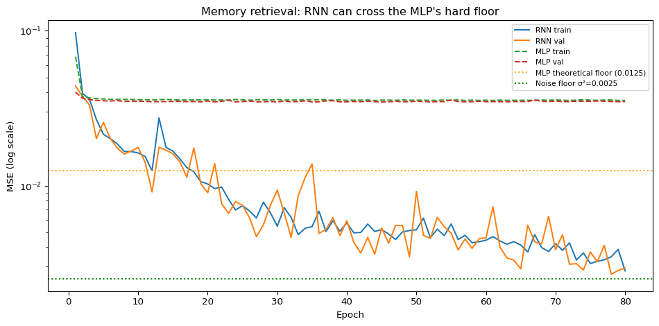
| 1 | MLP Baseline (window=5) | Last 5 steps only | 5σ²=0.0125 | 0.03490 |
| 2 | Naive (predict mean) | Nothing | Var(x₀)≈0.083 | 0.08360 |
Key takeaway:
The MLP’s failure here is not a matter of training or hyperparameters — it is a hard information-theoretic limit. No matter how wide or deep the MLP is, it cannot recover \(x_0\) from a window that doesn’t contain it. The RNN wins by design: its hidden state \(\mathbf{h}_1\) receives \(x_0\) directly at step 1 and can propagate it through to the final prediction.
This is precisely what “memory” means in sequence modelling: the ability to carry early information forward in \(\mathbf{h}_t\) until it is needed.
We use a simple recurrent neural network over words to classify short news headlines + blurbs into one of four topics:
This gives us a clean, realistic example where an RNN: - sees real text, not toy sequences - builds a compact representation of each headline - achieves high test accuracy (well above chance)
from torchtext.datasets import AG_NEWS
import torch
# Older text_classification API: returns (train_dataset, test_dataset)
train_dataset, test_dataset = AG_NEWS(root="data")
# Turn into simple lists of (label, text_tensor)
full_train = list(train_dataset)
full_test = list(test_dataset)
len(full_train), len(full_test)(120000, 7600)
torch.manual_seed(3151)
train_subset_size = 20_000
val_subset_size = 5_000
test_subset_size = 5_000
indices = torch.randperm(len(full_train))
train_idx = indices[:train_subset_size]
val_idx = indices[train_subset_size:train_subset_size + val_subset_size]
train_subset = [full_train[i] for i in train_idx]
val_subset = [full_train[i] for i in val_idx]
test_subset = full_test[:test_subset_size]
# Sanity check one example
train_subset[0](2,
tensor([ 156, 1949, 937, 5, 10297, 803, 145, 14, 28, 15,
16, 3, 52, 2, 10, 2, 1223, 156, 11, 56,
1032, 1766, 6, 22635, 860, 18, 15706, 17, 857, 5,
379, 2283, 43, 63, 5242, 25, 3, 101, 17, 10,
2291, 10297, 803, 2]))
Design choice
We trade a bit of accuracy for a big win in speed, so training fits comfortably into a live example or a short notebook run.
For this demo, AG_NEWS already provides token-id tensors in our torchtext environment. But sometimes we would have to:
This would give us a rectangular tensor (batch, max_len) of token IDs.
# AG_NEWS in this torchtext already returns token-id tensors,
# so we do NOT need to build a tokenizer/vocab manually here.
def encode(text, max_len=100):
# Compatibility: if a tensor is passed, pad/truncate directly
if isinstance(text, torch.Tensor):
return pad_to_max_len(text, max_len)
raise TypeError("Expected a tensor from AG_NEWS in this environment.")def pad_to_max_len(x, max_len=100):
# x is a 1D LongTensor of token IDs
if x.size(0) >= max_len:
return x[:max_len]
pad_len = max_len - x.size(0)
pad = torch.zeros(pad_len, dtype=torch.long) # 0 will act as "pad"/"<unk>"
return torch.cat([x, pad])
def prepare_dataset_tensor(examples, max_len=100):
xs, ys = [], []
for label, text_tensor in examples:
xs.append(pad_to_max_len(text_tensor, max_len))
ys.append(int(label))
return torch.stack(xs), torch.tensor(ys)
X_train, y_train = prepare_dataset_tensor(train_subset, max_len=100)
X_val, y_val = prepare_dataset_tensor(val_subset, max_len=100)
X_test, y_test = prepare_dataset_tensor(test_subset, max_len=100)
X_train.shape, y_train.shape(torch.Size([20000, 100]), torch.Size([20000]))
from torch.utils.data import TensorDataset, DataLoader
batch_size = 64
train_ds = TensorDataset(X_train, y_train)
val_ds = TensorDataset(X_val, y_val)
test_ds = TensorDataset(X_test, y_test)
train_loader = DataLoader(train_ds, batch_size=batch_size, shuffle=True)
val_loader = DataLoader(val_ds, batch_size=batch_size)
test_loader = DataLoader(test_ds, batch_size=batch_size)
# Infer vocab size from token-id tensors in train_subset
max_token_id = 0
for _, text_tensor in train_subset:
if len(text_tensor) > 0:
max_token_id = max(max_token_id, int(text_tensor.max().item()))
vocab_size = max_token_id + 1 # +1 because token IDs are 0-indexed
print("vocab_size =", vocab_size)vocab_size = 95812
We use a word-level RNN:
nn.Embedding turns token IDs into vectorsnn.GRU reads the sequence left→right and right→leftThis gives a single vector per headline that captures its topic.
import torch.nn as nn
class NewsRNN(nn.Module):
def __init__(self, vocab_size, embed_dim=128,
hidden_size=64, num_classes=4):
super().__init__()
self.embed = nn.Embedding(vocab_size, embed_dim, padding_idx=0)
self.gru = nn.GRU(embed_dim, hidden_size,
batch_first=True, bidirectional=True)
self.fc = nn.Linear(hidden_size * 2, num_classes)
def forward(self, x):
# x: (batch, seq_len)
emb = self.embed(x) # (batch, seq_len, embed_dim)
output, h_n = self.gru(emb) # h_n: (2, batch, hidden_size)
h_last = torch.cat([h_n[0], h_n[1]], dim=1) # (batch, 2 * hidden)
logits = self.fc(h_last)
return logits
device = torch.device("cuda" if torch.cuda.is_available() else "cpu")
model = NewsRNN(vocab_size=vocab_size).to(device)import torch.optim as optim
criterion = nn.CrossEntropyLoss()
optimizer = optim.Adam(model.parameters(), lr=1e-3)
def run_epoch(loader, train=True):
if train:
model.train()
else:
model.eval()
total_loss, total_correct, total_examples = 0.0, 0, 0
for X, y in loader:
X, y = X.to(device), y.to(device)
if train:
optimizer.zero_grad()
logits = model(X)
loss = criterion(logits, y)
if train:
loss.backward()
optimizer.step()
total_loss += loss.item() * X.size(0)
preds = logits.argmax(dim=1)
total_correct += (preds == y).sum().item()
total_examples += X.size(0)
return total_loss / total_examples, total_correct / total_examples
history = {"train_loss": [], "val_loss": [],
"train_acc": [], "val_acc": []}
for epoch in range(1, 9):
train_loss, train_acc = run_epoch(train_loader, train=True)
val_loss, val_acc = run_epoch(val_loader, train=False)
history["train_loss"].append(train_loss)
history["val_loss"].append(val_loss)
history["train_acc"].append(train_acc)
history["val_acc"].append(val_acc)
print(f"Epoch {epoch}: "
f"train_acc={train_acc:.3f}, val_acc={val_acc:.3f}, "
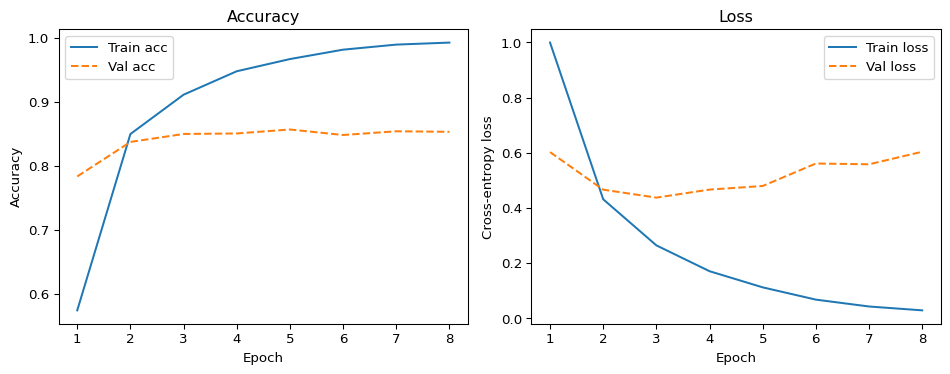
f"train_loss={train_loss:.3f}, val_loss={val_loss:.3f}")Epoch 1: train_acc=0.575, val_acc=0.783, train_loss=1.000, val_loss=0.602
Epoch 2: train_acc=0.850, val_acc=0.837, train_loss=0.431, val_loss=0.466
Epoch 3: train_acc=0.911, val_acc=0.850, train_loss=0.264, val_loss=0.437
Epoch 4: train_acc=0.947, val_acc=0.850, train_loss=0.170, val_loss=0.466
Epoch 5: train_acc=0.966, val_acc=0.857, train_loss=0.112, val_loss=0.479
Epoch 6: train_acc=0.981, val_acc=0.848, train_loss=0.067, val_loss=0.561
Epoch 7: train_acc=0.989, val_acc=0.854, train_loss=0.042, val_loss=0.558
Epoch 8: train_acc=0.992, val_acc=0.853, train_loss=0.028, val_loss=0.604
In practice you would pre-run this once and keep the printed output and plots, rather than re-training live every time.
import matplotlib.pyplot as plt
epochs = range(1, len(history["train_acc"]) + 1)
fig, axes = plt.subplots(1, 2, figsize=(10, 4))
# Accuracy
axes[0].plot(epochs, history["train_acc"], label="Train acc")
axes[0].plot(epochs, history["val_acc"], label="Val acc", linestyle="--")
axes[0].set_xlabel("Epoch")
axes[0].set_ylabel("Accuracy")
axes[0].set_title("Accuracy")
axes[0].legend()
# Loss
axes[1].plot(epochs, history["train_loss"], label="Train loss")
axes[1].plot(epochs, history["val_loss"], label="Val loss", linestyle="--")
axes[1].set_xlabel("Epoch")
axes[1].set_ylabel("Cross-entropy loss")
axes[1].set_title("Loss")
axes[1].legend()
plt.tight_layout()
plt.show()
The right metric depends on the task type:
| Task | Typical metric | Notes |
|---|---|---|
| Sequence regression | MSE, MAE | Per-step or final-step |
| Sequence classification | Accuracy, F1 | Standard classification metrics |
| Language modelling | Perplexity | \(\exp(\text{avg cross-entropy per token})\) |
| Sequence labelling | Token-level F1 | Must account for each step |
Goal alignment:
Don’t report only training loss!
For sequence models, the gap between train and val loss is a direct indicator of whether the model is memorising the training sequences or learning the underlying pattern.
Let’s be explicit about the known limitations:
Preview of M49:
LSTMs (Long Short-Term Memory) and GRUs add learnable gates that solve problems 1 and 3. They do not magically fix exploding gradients, but the forget/input/output gates can keep relevant information alive for hundreds of steps.
Even “simple” RNN applications carry real-world risks:
1. Training data bias propagates through time:
2. Language identification can be a proxy for national origin or ethnicity:
3. Privacy in sequence data :
Simple mitigation check: Before deploying any sequence model, ask: What group differences does the training data encode? Could the model’s predictions be used to discriminate or surveil?
Q1. A vanilla RNN is trained to classify 5-word sentences as positive or negative sentiment.
The input vocabulary has 10,000 words. Each word is embedded into a 50-dimensional vector. The hidden size is 64.
Which of the following is true about the weight matrix \(W_{hh}\)?
Its shape is \((50, 64)\) — it connects the input to the hidden state.
Its shape is \((64, 64)\) — it connects the hidden state to itself, and is shared across all 5 time steps.
Its shape is \((64, 64)\) — there is a separate copy for each of the 5 time steps.
Its shape is \((10000, 64)\) — it encodes each word into a hidden state.
Q2. Short answer: Explain in 2–3 sentences why Backpropagation Through Time (BPTT) can lead to vanishing gradients, and state which parameter is most responsible.
(Write your answer before reading the hint below.)
Hint / model answer:
In BPTT, the gradient of the loss with respect to an early hidden state \(\mathbf{h}_1\) involves multiplying \(T-1\) Jacobian factors, each of the form \(\text{diag}(f') \cdot W_{hh}\).
If the spectral radius of \(W_{hh}\) is less than 1, this product shrinks exponentially with \(T\) — the gradient vanishes. The matrix \(W_{hh}\) (the hidden-to-hidden weight matrix) is most responsible, because it is the term being raised to a power proportional to the sequence length.
Q3. In Worked Example 1 (memory retrieval), the MLP is given a deeper hidden layer and trained for 3× as many epochs. Its validation MSE barely improves.
Why? Choose all that apply.
The MLP is not wide enough to fit the data.
The MLP’s window does not contain \(x_0\), so no amount of additional parameters or training can recover the missing information.
The task requires an inductive bias that the MLP lacks: the ability to propagate information from early time steps to the final prediction.
Gradient clipping is preventing the MLP from converging.
Q4. Numeric question: An RNN has:
How many total trainable parameters does this vanilla RNN have?
(Assume biases are included for both the recurrent layer and the output layer.)
(Hint: count \(W_{xh}\), \(W_{hh}\), \(\mathbf{b}_h\), \(W_{hy}\), \(\mathbf{b}_y\) separately.)
