CSCI 3151 — Foundations of Machine Learning
By the end of this module, you should be able to:
👉 Key idea: images are highly structured 👈:

What went wrong?
Among other problems, the model has no built-in notion that a digit shifted by one pixel is “the same” object. It must learn that invariance from scratch.
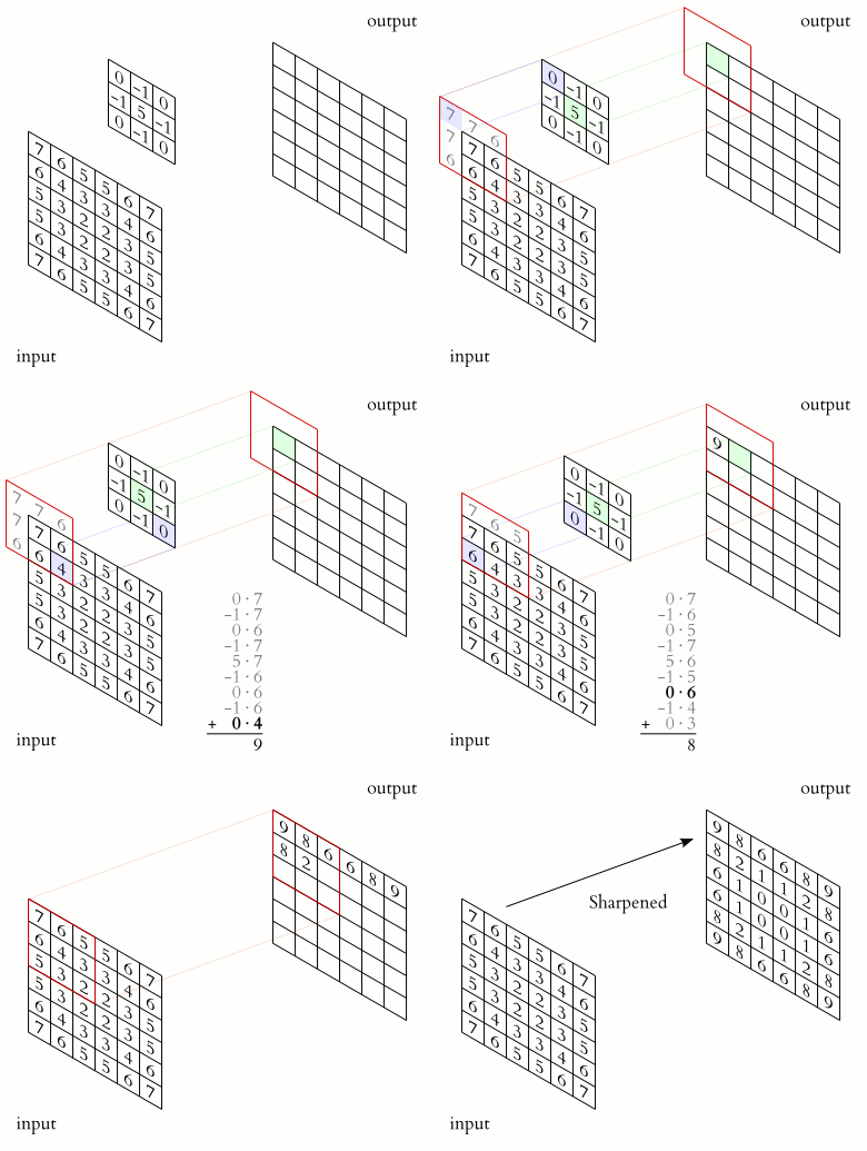
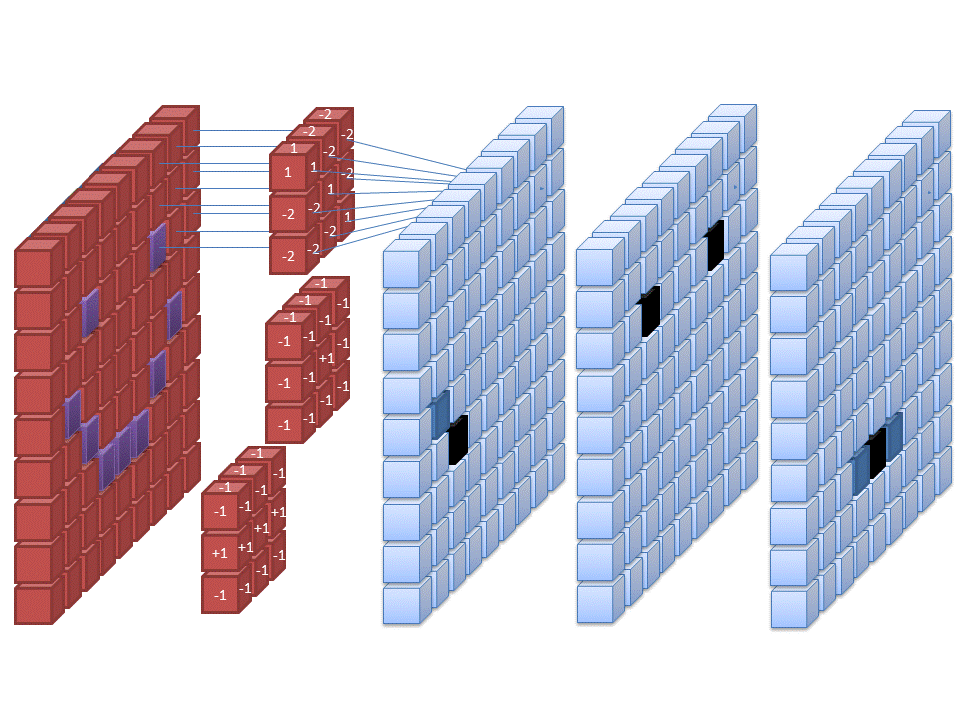
Convolution layer:

From here
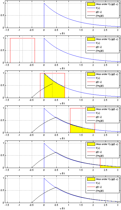
Intuition
For 1D signals \(x\) (input) and \(w\) (kernel), the discrete convolution is:
\[ (y = x * w)[i] = \sum_{k} x[i - k] w[k] \]
From here
In deep learning libraries, we often use cross-correlation instead:
\[ (y = x \star w)[i] = \sum_{k} x[i + k] w[k] \]
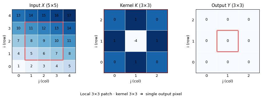
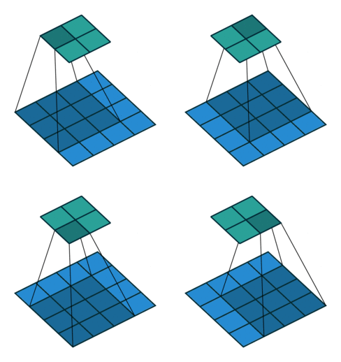
For single-channel 2D input \(X \in \mathbb{R}^{H \times W}\) and kernel \(K \in \mathbb{R}^{k_H \times k_W}\), ignoring stride & padding:
\[ Y[i, j] = (X \star K)[i, j] = \sum_{u=0}^{k_H-1} \sum_{v=0}^{k_W-1} K[u, v] \, X[i + u, j + v] \]

For input \(H \times W\), kernel \(k_H \times k_W\), padding \(p_H, p_W\), stride \(s_H, s_W\):
\[ H_{ \text{out}} = \left\lfloor \frac{H + 2p_H - k_H}{s_H} \right\rfloor + 1,\quad W_{ \text{out}} = \left\lfloor \frac{W + 2p_W - k_W}{s_W} \right\rfloor + 1 \]
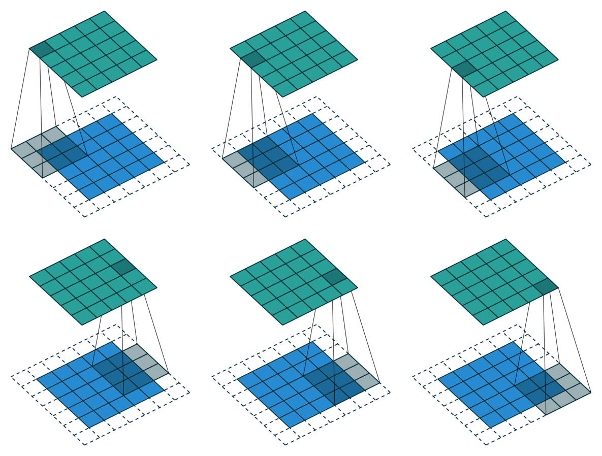
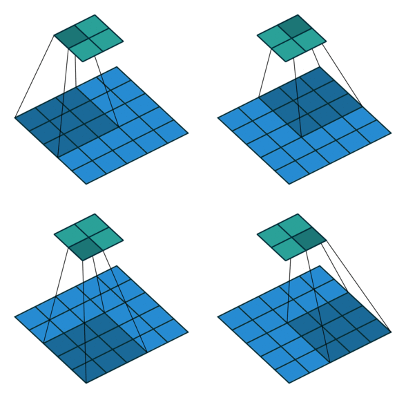
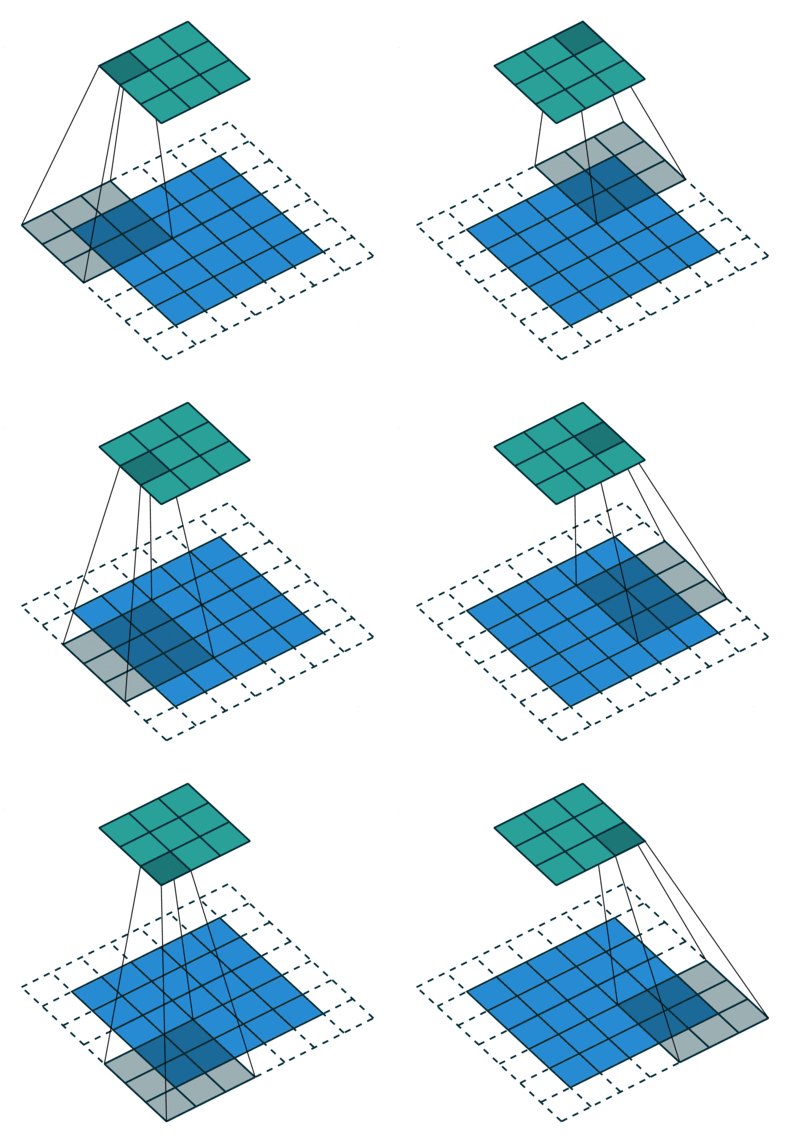
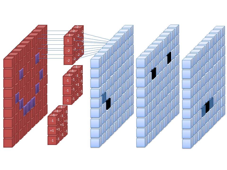
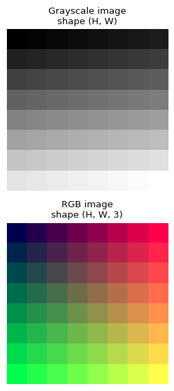
For multi-channel input (e.g., RGB):
\[ Y[i, j] = \sum_{c=1}^{C_\text{in}} \sum_{u,v} K[c, u, v] \, X[c, i+u, j+v] \]
To produce \(C_\text{out}\) feature maps, we use \(C_\text{out}\) filters:

From here
Consider 32×32 RGB images (\(C=3, H=W=32\)) and a layer with 64 hidden units:
| Layer type | Parameters (approx) |
|---|---|
| MLP dense | 196,608 |
| Conv (3×3, 64 filters) | 1,728 |
Tip
Convs are much more parameter-efficient for images.
Ideally, if we shift the input, the feature map should shift in the same way.
Simplify to 1D and cross-correlation:
Define shift operator: \((T_\delta x)[i] = x[i - \delta]\).
Claim (equivariance):
\[ (T_\delta x \star w)[i] = T_\delta (x \star w)[i] = y[i - \delta] \]
Proof sketch:
\[ \begin{aligned} (T_\delta x \star w)[i] &= \sum_k (T_\delta x)[i + k] w[k] \\ &= \sum_k x[i + k - \delta] w[k] \\ &= \sum_k x[(i - \delta) + k] w[k] \\ &= (x \star w)[i - \delta] = y[i - \delta] = T_\delta y[i]. \end{aligned} \]
So convolution (or cross-correlation) is translation equivariant: shift in, shift out.
Pooling layers reduce spatial resolution by summarizing local neighbourhoods.
Max pooling
\[ Y[i, j] = \max_{(u,v) \in \text{window}} X[i + u, j + v] \]
Average pooling
\[ Y[i, j] = \frac{1}{|W|} \sum_{(u,v)\in W} X[i + u, j + v] \]
Pooling window size & stride (often same) control how much invariance & downsampling.
Imagine a CNN for handwritten digit recognition:
Warning
Because the 7×7, stride-7 pooling windows collapse many different input locations into the same pooled value (and, after enough pooling, to a 1×1 map there’s only one cell), 👉 the network’s later layers see exactly the same representation no matter where the pattern appeared, making it effectively invariant to location 👈.
Consequences:
Takeaway
Pooling is powerful, but too much invariance is also bad.
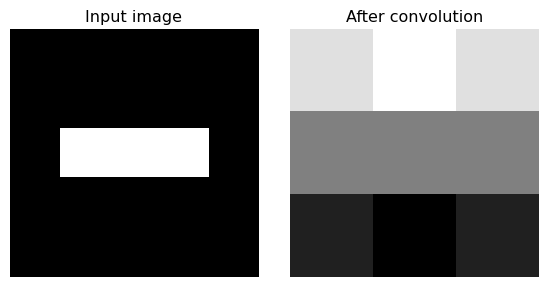
We’ll build a tiny “image” and a simple edge-detection kernel.
🥅 Goal
import numpy as np
import pandas as pd
import matplotlib.pyplot as plt
# Tiny 5x5 "image" with a bright horizontal bar
img = np.array([
[0, 0, 0, 0, 0],
[0, 0, 0, 0, 0],
[0, 1, 1, 1, 0],
[0, 0, 0, 0, 0],
[0, 0, 0, 0, 0],
], dtype=float)
# Simple horizontal edge detector (Sobel-like)
kernel = np.array([
[-1, -2, -1],
[ 0, 0, 0],
[ 1, 2, 1],
], dtype=float)
img_df = pd.DataFrame(img)
kernel_df = pd.DataFrame(kernel)
print("Our image:")
img_dfOur image:
| 0 | 1 | 2 | 3 | 4 | |
|---|---|---|---|---|---|
| 0 | 0.0 | 0.0 | 0.0 | 0.0 | 0.0 |
| 1 | 0.0 | 0.0 | 0.0 | 0.0 | 0.0 |
| 2 | 0.0 | 1.0 | 1.0 | 1.0 | 0.0 |
| 3 | 0.0 | 0.0 | 0.0 | 0.0 | 0.0 |
| 4 | 0.0 | 0.0 | 0.0 | 0.0 | 0.0 |
def conv2d_valid(x, k):
H, W = x.shape
kH, kW = k.shape
out = np.zeros((H - kH + 1, W - kW + 1))
for i in range(out.shape[0]):
for j in range(out.shape[1]):
patch = x[i:i+kH, j:j+kW]
out[i, j] = np.sum(patch * k)
return out
edge = conv2d_valid(img, kernel)
edge_df = pd.DataFrame(edge)
print("Our edge-detecting kernel:")
edge_dfOur edge-detecting kernel:
| 0 | 1 | 2 | |
|---|---|---|---|
| 0 | 3.0 | 4.0 | 3.0 |
| 1 | 0.0 | 0.0 | 0.0 |
| 2 | -3.0 | -4.0 | -3.0 |
def max_pool2d(x, pool_size=2, stride=2):
H, W = x.shape
out_H = (H - pool_size) // stride + 1
out_W = (W - pool_size) // stride + 1
out = np.zeros((out_H, out_W))
for i in range(out_H):
for j in range(out_W):
patch = x[i*stride:i*stride+pool_size,
j*stride:j*stride+pool_size]
out[i, j] = patch.max()
return out
pooled = max_pool2d(edge, pool_size=2, stride=1)
pd.DataFrame(pooled)| 0 | 1 | |
|---|---|---|
| 0 | 4.0 | 4.0 |
| 1 | 0.0 | 0.0 |

Note
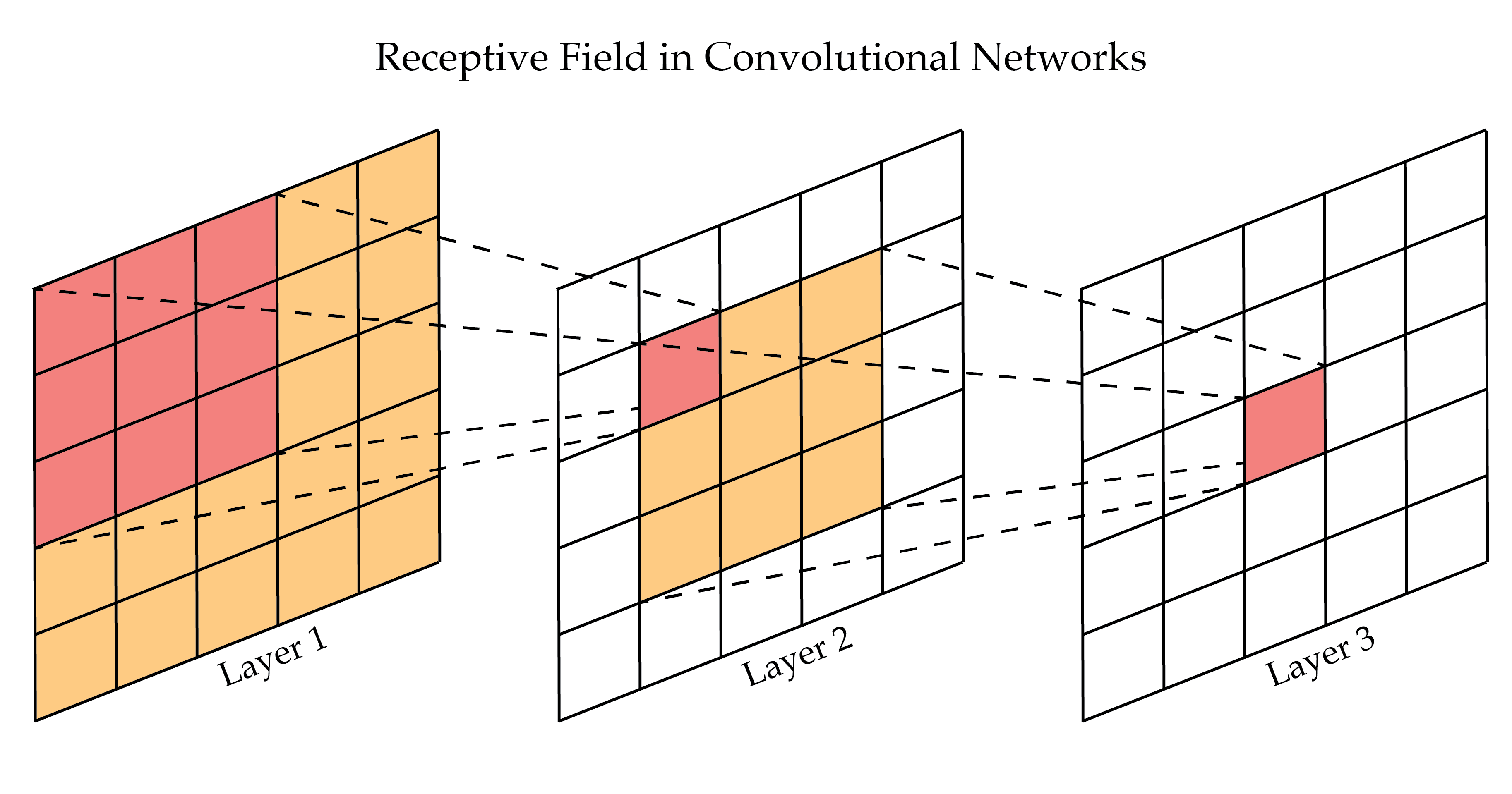
stride=2?Receptive field of a unit = region of the input it “sees.”
Mini-table example
| Layer | Kernel / stride | Effective RF size |
|---|---|---|
| Conv1 | 3×3 / 1 | 3×3 |
| Conv2 | 3×3 / 1 | 5×5 |
| MaxPool (2×2) | 2×2 / 2 | 6×6 (coarser grid) |
Receptive fields help explain how deep layers can “see” entire objects.
From here
Most CNNs are made of a few repeating pieces:
Conv2d(in_channels, out_channels, kernel_size, stride, padding)
Conv2dExample pattern (“conv block”):
🥅 Goal
We’ll train only for a few epochs on a small subset so this runs quickly in a notebook.
import torch
from torch import nn
from torch.utils.data import DataLoader, Subset
import torchvision
from torchvision import datasets, transforms
import numpy as np
import pandas as pd
import matplotlib.pyplot as plt
device = torch.device("cuda" if torch.cuda.is_available() else "cpu")
transform = transforms.Compose([
transforms.ToTensor(),
transforms.Normalize((0.5, 0.5, 0.5),
(0.5, 0.5, 0.5)),
])
train_full = datasets.CIFAR10(root="data", train=True, download=True, transform=transform)
test_full = datasets.CIFAR10(root="data", train=False, download=True, transform=transform)
# Use a small subset to keep training fast (e.g., 5000 train, 1000 test)
np.random.seed(0)
train_indices = np.random.choice(len(train_full), size=5000, replace=False)
test_indices = np.random.choice(len(test_full), size=1000, replace=False)
train_subset = Subset(train_full, train_indices)
test_subset = Subset(test_full, test_indices)
train_loader = DataLoader(train_subset, batch_size=64, shuffle=True)
test_loader = DataLoader(test_subset, batch_size=64, shuffle=False)class SmallCNN(nn.Module):
def __init__(self):
super().__init__()
self.features = nn.Sequential(
nn.Conv2d(3, 32, kernel_size=3, padding=1),
nn.ReLU(),
nn.MaxPool2d(kernel_size=2), # 32x16x16
nn.Conv2d(32, 64, kernel_size=3, padding=1),
nn.ReLU(),
nn.MaxPool2d(kernel_size=2), # 64x8x8
)
self.classifier = nn.Sequential(
nn.Flatten(),
nn.Linear(64 * 8 * 8, 10),
)
def forward(self, x):
x = self.features(x)
x = self.classifier(x)
return x
cnn = SmallCNN().to(device)def train_epoch(model, loader, optimizer, loss_fn):
model.train()
total_loss = 0.0
correct = 0
total = 0
for x, y in loader:
x, y = x.to(device), y.to(device)
optimizer.zero_grad()
logits = model(x)
loss = loss_fn(logits, y)
loss.backward()
optimizer.step()
total_loss += loss.item() * x.size(0)
preds = logits.argmax(dim=1)
correct += (preds == y).sum().item()
total += x.size(0)
return total_loss / total, correct / total
@torch.no_grad()
def evaluate(model, loader, loss_fn):
model.eval()
total_loss = 0.0
correct = 0
total = 0
for x, y in loader:
x, y = x.to(device), y.to(device)
logits = model(x)
loss = loss_fn(logits, y)
total_loss += loss.item() * x.size(0)
preds = logits.argmax(dim=1)
correct += (preds == y).sum().item()
total += x.size(0)
return total_loss / total, correct / totaldef run_experiment(model, train_loader, test_loader, epochs=5, lr=1e-3):
loss_fn = nn.CrossEntropyLoss()
optimizer = torch.optim.Adam(model.parameters(), lr=lr)
history = {"train_loss": [], "train_acc": [],
"test_loss": [], "test_acc": []}
for epoch in range(epochs):
tl, ta = train_epoch(model, train_loader, optimizer, loss_fn)
vl, va = evaluate(model, test_loader, loss_fn)
history["train_loss"].append(tl)
history["train_acc"].append(ta)
history["test_loss"].append(vl)
history["test_acc"].append(va)
print(f"Epoch {epoch+1}: "
f"train_acc={ta:.3f}, test_acc={va:.3f}")
return history
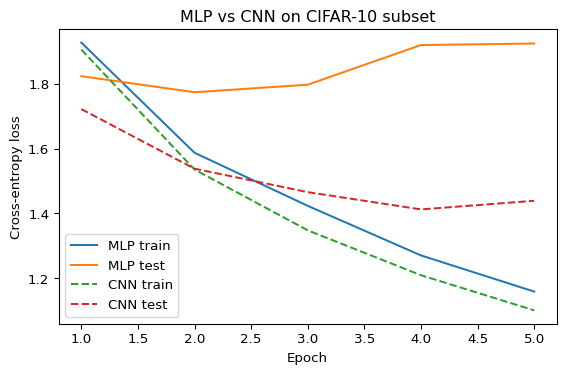
mlp_hist = run_experiment(mlp, train_loader, test_loader, epochs=5, lr=1e-3)
cnn_hist = run_experiment(cnn, train_loader, test_loader, epochs=5, lr=1e-3)Epoch 1: train_acc=0.330, test_acc=0.369
Epoch 2: train_acc=0.447, test_acc=0.392
Epoch 3: train_acc=0.507, test_acc=0.373
Epoch 4: train_acc=0.561, test_acc=0.382
Epoch 5: train_acc=0.602, test_acc=0.399
Epoch 1: train_acc=0.307, test_acc=0.363
Epoch 2: train_acc=0.455, test_acc=0.452
Epoch 3: train_acc=0.527, test_acc=0.488
Epoch 4: train_acc=0.576, test_acc=0.498
Epoch 5: train_acc=0.608, test_acc=0.495
def count_params(model):
return sum(p.numel() for p in model.parameters())
summary = pd.DataFrame({
"model": ["MLP", "CNN"],
"params": [count_params(mlp), count_params(cnn)],
"train_acc": [mlp_hist["train_acc"][-1],
cnn_hist["train_acc"][-1]],
"test_acc": [mlp_hist["test_acc"][-1],
cnn_hist["test_acc"][-1]],
})
summary| model | params | train_acc | test_acc | |
|---|---|---|---|---|
| 0 | MLP | 1578506 | 0.6022 | 0.399 |
| 1 | CNN | 60362 | 0.6078 | 0.495 |
epochs = range(1, len(mlp_hist["train_loss"]) + 1)
plt.figure(figsize=(6, 4))
plt.plot(epochs, mlp_hist["train_loss"], label="MLP train")
plt.plot(epochs, mlp_hist["test_loss"], label="MLP test")
plt.plot(epochs, cnn_hist["train_loss"], label="CNN train", linestyle="--")
plt.plot(epochs, cnn_hist["test_loss"], label="CNN test", linestyle="--")
plt.xlabel("Epoch")
plt.ylabel("Cross-entropy loss")
plt.title("MLP vs CNN on CIFAR-10 subset")
plt.legend()
plt.tight_layout()

✏️ Ask yourself
Imagine CNN-based classification, e.g.:
A pre-filter for organizing photos into broad categories in a consumer app.
For more sensitive applications (e.g., medical imaging, safety-critical robotics):
Warning
CNNs provide better feature extraction for images than MLPs, but the evaluation metric must still match the real-world cost of errors.
When applying CNNs to real images, we must think beyond accuracy:
CNN-style architectures show up in:
Connections:
CNNs bake in strong assumptions:
These are inductive biases:
Tip
Thinking in terms of “what invariances / equivariances does my model assume?” is a powerful design habit.
Q1: You apply a conv layer with:
What is the output shape?
A. (16, 30, 30)
B. (16, 32, 32)
C. (3, 32, 32)
D. (16, 34, 34)
Q2 (short) — equivariance vs invariance
In one sentence each:
Q3 (MCQ) — pooling
Which of the following is not a good reason to use pooling?
A. To reduce spatial resolution and computation
B. To introduce local translation invariance
C. To guarantee that the network never overfits
D. To gradually increase receptive field size
Q4 (short numeric) — receptive field size
You stack:
What is the receptive field size (in terms of input pixels) of a unit after the max pool?
(Assume square kernels and ignore boundary effects.)