M41: Embeddings for Images, Text, and Graphs

CSCI 3151 — Foundations of Machine Learning

Frank Rudzicz

Table of contents

• Conceptual scaffold
• Worked example 1: Gigaword
• Worked example 2: CIFAR-10
• Summary

Learning outcomes

By the end of this module, you should be able to:

1. Explain what an embedding is and why we use embeddings across modalities.
2. Compare common embedding approaches for text, images, and graphs at a high level.
3. Use pre-trained embeddings (for text and images) to build simple downstream models or visualizations.
4. Evaluate embedding quality using downstream tasks (e.g., k-NN classification, retrieval).
5. Identify basic risks and biases in learned embeddings and describe simple mitigation strategies.

Motivation: why embeddings?

• Many ML models don’t operate directly on:
  • Raw text, pixels, nodes, users, items, …
• Instead, they operate on vectors in \(\mathbb{R}^d\):
  • Each object → a point in a continuous space
• This gives us:
  • A common language for similarity (distances, angles)
  • The ability to plug into generic tools:
    • Linear models, k-NN, clustering, visualization, retrieval

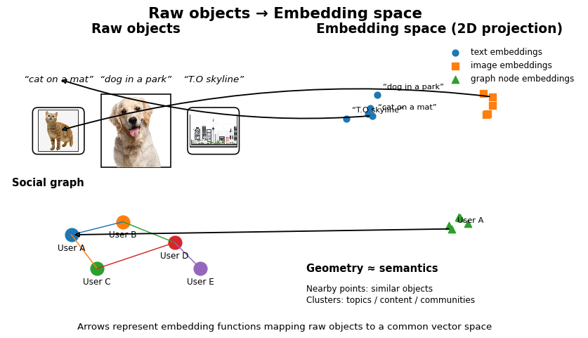
Big idea: Design (or learn) a function

\[ f: \text{objects} \to \mathbb{R}^d \]

so that geometry ≈ semantics:

• Nearby points → “similar” objects
  
• Directions capture relations (e.g., gender, tense, topic, style)

Conceptual scaffold

Key definitions

Representation (M40)

• Any way of turning raw data into a form a model can work with
  e.g., bag-of-words vectors, pixels, spectrograms, hand-crafted features

Embedding

• A representation that:
  • Lives in a fixed-dimensional vector space \(\mathbb{R}^d\)
  • Is typically learned, not hand-crafted
  • Is often dense (most dimensions nonzero) and low-ish-dimensional

\[ \text{embedding} = f(x) \in \mathbb{R}^d \]

Embedding space

• The whole set of points \(\{ f(x) : x \in \mathcal{X} \}\)
  
• Equipped with a similarity / distance notion:
  • Euclidean distance, cosine similarity, dot product, etc.

Visualizing embeddings

❌ Anti-example: misleading “embeddings”

Scenario:

• You download a black-box “text embedding” model pre-trained on web data.
• You use its embeddings to rank job applicants based on their cover letters:
  • Compute embedding for each cover letter
  • Compute cosine similarity to a “prototype” embedding built from your favourite past hires
  • Hire the top-\(k\) most similar applicants

Problems / violations:

• The embedding model likely encodes historical bias:
  • Stereotypes about gender, race, etc.
• “Similarity to past hires” may reinforce existing inequalities.
• No calibration or validation on your specific task.
• No controls for protected attributes or their proxies.

Warning

Key lesson: nicely structured embedding space ≠ fair or appropriate for any downstream decision.

Embeddings as functions

At a high level:

• Text: \(f_\text{text}(\text{token or sentence}) \to \mathbb{R}^{d_\text{text}}\)
• Images: \(f_\text{img}( \text{pixel array}) \to \mathbb{R}^{d_\text{img}}\)
• Graphs: \(f_\text{graph}( \text{node}) \to \mathbb{R}^{d_\text{graph}}\)

Common patterns:

• \(f\) often comes from a neural network:
  • Text: word2vec, GloVe, BERT, sentence transformers
  • Images: CNNs, vision transformers
  • Graphs: DeepWalk, node2vec, graph neural networks (GNNs)

Key design choices:

• What structure do we want to preserve?
  • Local neighbours? Global distances? Node communities? Temporal order?
• What objective do we use?
  • Predict context words, classify images, reconstruct neighbours, contrastive learning, …

Similarity metrics in embedding spaces

Let \(u, v \in \mathbb{R}^d\) be embeddings.

• Euclidean distance

\[ d_\text{L2}(u, v) = \|u - v\|_2 \]

• Cosine similarity

\[ \text{cos_sim}(u, v) = \frac{u^\top v}{\|u\|_2 \|v\|_2} \]

• Dot product

\[ u^\top v \]

Why cosine?

• Often we care about direction more than magnitude.
• In high dimensions, raw distances can be less informative; norms may vary a lot.

Design rule:

• If embeddings are used with k-NN / clustering, choose a similarity consistent with how they were trained (often cosine or dot product).

🔬 Skip-gram with negative sampling (SGNS)

Very popular text embeddings (e.g., word2vec) are trained with a contrastive objective:

• We want words to be similar to their true context words and dissimilar to random words.

For a target word \(w\) and a context word \(c\):

• Let \(v_w\) and \(v_c\) be their embedding vectors.
• SGNS objective for one (target, context) pair:

\[ \log \sigma(v_w^\top v_c) + \sum_{i=1}^k \mathbb{E}_{n_i \sim P_n} \left[\log \sigma(-v_w^\top v_{n_i})\right] \]

• \(\sigma\) is the logistic sigmoid.
• First term: encourage \(v_w\) close to \(v_c\).
• Second term: for \(k\) “negative” samples \(n_i\), push \(v_w\) away from unrelated words.

Interpretation:

• SGNS learns embeddings where co-occurring words have large dot products.
• Can be shown (roughly) to factorize a shifted PMI (pointwise mutual information) matrix between word and context.

You don’t need the full derivation here—but it’s a good example of how objectives shape geometry.

Text embeddings: big picture

Three broad generations:

1. Sparse count-based representations
   • Bag-of-words, TF-IDF, n-grams (Manning, Raghavan, and Schütze 2008)
   • Very high-dimensional, mostly zeros
2. 👉 Dense word embeddings
   • word2vec (Mikolov et al. 2013), GloVe (Pennington, Socher, and Manning 2014), fastText (Bojanowski et al. 2017)
   • Each token → a dense vector with semantic structure
3. Contextual embeddings
   • ELMo (Peters et al. 2018), BERT (Devlin et al. 2019), GPT (Radford et al. 2018), etc.
   • Same token can have different vectors depending on context
   • Embeddings come from deep sequence models (transformers)

Worked example 1: Gigaword

Exploring word embeddings (GloVe / word2vec)

Goal:

• Load pre-trained word embeddings.
• Explore:
  • Nearest neighbours (semantic similarity)
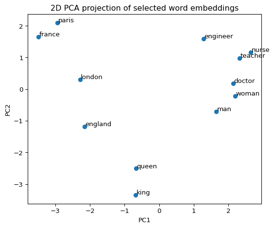
  • Simple analogies (e.g., king − man + woman ≈ queen)
  • 2D visualization via PCA or t-SNE.

Dataset:

• Pre-trained embedding model trained on a large open corpus, e.g.:
  • glove-wiki-gigaword-50 (GloVe on Wikipedia + Gigaword)
  • or a similar word2vec model

Note

These models are not trained in this module; we reuse them as a learned embedding space. See 🔗gensim

⚠️ I had trouble using pip install gensim, so I had to conda install -c conda-forge gensim. Your kilometrage may vary.

Loading and probing a text embedding model

import numpy as np
import pandas as pd
import matplotlib.pyplot as plt
from sklearn.decomposition import PCA

# Optional: pip install gensim before this
import gensim.downloader as api

# Load a small pre-trained GloVe model (50-dimensional)
glove = api.load("glove-wiki-gigaword-50")

# A small, hand-picked vocabulary to explore
words = [
    "king", "queen", "man", "woman",
    "doctor", "nurse", "engineer", "teacher",
    "paris", "france", "london", "england"
]

vectors = np.vstack([glove[w] for w in words])
vec_df = pd.DataFrame(vectors, index=words)
vec_df.head()

	0	1	2	3	4	5	6	7	8	9	...	40	41	42	43	44	45	46	47	48	49
king	0.504510	0.68607	-0.59517	-0.022801	0.60046	-0.13498	-0.08813	0.47377	-0.617980	-0.31012	...	0.401020	1.16850	-1.01370	-0.215850	-0.15155	0.78321	-0.91241	-1.610600	-0.644260	-0.51042
queen	0.378540	1.82330	-1.26480	-0.104300	0.35829	0.60029	-0.17538	0.83767	-0.056798	-0.75795	...	0.459460	0.25302	-0.17837	-0.733980	-0.20025	0.23470	-0.56095	-2.283900	0.009275	-0.60284
man	-0.094386	0.43007	-0.17224	-0.455290	1.64470	0.40335	-0.37263	0.25071	-0.105880	0.10778	...	-0.086264	0.62549	-0.05760	0.293750	0.66005	-0.53115	-0.48233	-0.979250	0.531350	-0.11725
woman	-0.181530	0.64827	-0.58210	-0.494510	1.54150	1.34500	-0.43305	0.58059	0.355560	-0.25184	...	-0.251740	0.42123	0.48616	0.022325	0.55760	-0.85223	-0.23073	-1.313800	0.487640	-0.10467
doctor	0.669990	0.11698	-0.46322	-0.900120	0.56560	0.48980	-0.26031	0.71268	0.623380	0.02785	...	0.410300	0.71996	-0.16293	0.291060	0.47188	-0.15121	0.36688	-0.089993	0.377780	0.59818

5 rows × 50 columns

2D visualization of word embeddings

pca = PCA(n_components=2)
coords_2d = pca.fit_transform(vectors)

viz_df = pd.DataFrame(coords_2d, columns=["pc1", "pc2"])
viz_df["word"] = words
viz_df

	pc1	pc2	word
0	-0.676859	-3.344144	king
1	-0.665034	-2.508571	queen
2	1.648064	-0.703755	man
3	2.186551	-0.212141	woman
4	2.134742	0.177946	doctor
5	2.643437	1.157769	nurse
6	1.279328	1.590130	engineer
7	2.315087	0.976006	teacher
8	-2.933943	2.095312	paris
9	-3.487676	1.649457	france
10	-2.284191	0.305338	london
11	-2.159503	-1.183347	england

plt.figure(figsize=(6, 5))
plt.scatter(coords_2d[:, 0], coords_2d[:, 1])

for (x, y, word) in zip(coords_2d[:, 0], coords_2d[:, 1], words):
    plt.text(x + 0.02, y + 0.02, word)

plt.xlabel("PC1")
plt.ylabel("PC2")
plt.title("2D PCA projection of selected word embeddings")
plt.tight_layout()
plt.show()

Nearest neighbours and analogies

def top_similar(query, top_n=5):
    return glove.most_similar(query, topn=top_n)

print("Nearest neighbours of 'doctor':")
for word, score in top_similar("doctor"):
    print(f"{word:12s}  cos_sim={score: .3f}")

Nearest neighbours of 'doctor':
nurse         cos_sim= 0.798
physician     cos_sim= 0.797
patient       cos_sim= 0.761
child         cos_sim= 0.756
teacher       cos_sim= 0.754

analogies = glove.most_similar(
    positive=["king", "woman"],
    negative=["man"],
    topn=5
)
print("king - man + woman ≈ ?")
for word, score in analogies:
    print(f"{word:12s}  cos_sim={score: .3f}")

king - man + woman ≈ ?
queen         cos_sim= 0.852
throne        cos_sim= 0.766
prince        cos_sim= 0.759
daughter      cos_sim= 0.747
elizabeth     cos_sim= 0.746

Design choice / subtlety:

• Analogy results are not always “correct”:
  • They reflect biases and statistics in the training corpus.
• Still, they are a useful sanity check:
  • Do we see gender, country–capital, or profession clusters emerging?

Evaluating text embeddings (quick lens)

Typical checks:

• Neighbour quality:
  • Are nearest neighbours semantically coherent?
• Analogy tests (word2vec famous examples):
  • king - man + woman ≈ queen
  • paris - france + italy ≈ rome
• Downstream performance:
  • Average word embeddings for sentences and run:
    • \(k\)-NN classification
    • Simple logistic regression
• Limitations:
  • Word embeddings alone cannot capture complex syntax or long-range context.
  • Biases from the corpus can be visible in analogies and neighbours.

Worked example 2: CIFAR-10

Image embeddings: big picture

For images, embeddings typically come from CNNs or vision transformers.

Pipeline:

1. Raw image \(x\) (e.g., \(3 \times 32 \times 32\) for CIFAR-10).
2. Pass through a trained network \(f_\theta\).
3. Take the penultimate layer output as embedding:

\[ z = f_\theta(x) \in \mathbb{R}^d \]

Re-use \(z\) for:

• Linear probes (train a simple classifier on top)
• \(k\)-NN classification / retrieval
• Visualization (PCA, t-SNE, UMAP on \(z\))
• Transfer learning to new tasks

In this example, we’ll use a pre-trained ResNet-18 and the CIFAR-10 dataset.

CIFAR-10 embeddings with ResNet-18

Goal:

• Use a pre-trained ResNet-18 (ImageNet) as an embedding extractor.
• Extract embeddings for a small subset of CIFAR-10 images.
• Visualize them in 2D and run a simple \(k\)-NN classifier in embedding space.

Dataset:

• CIFAR-10 (open, widely used):
  • 10 classes: airplane, automobile, bird, cat, deer, dog, frog, horse, ship, truck
  • Images: 32×32 RGB

We’ll work with a small subset (e.g., 500 images) to keep things lightweight.

Loading CIFAR-10 and a pre-trained ResNet-18

import torch
from torch import nn
from torchvision import datasets, transforms, models
from torch.utils.data import DataLoader, Subset

# Basic transform: resize to 224x224 and normalize like ImageNet
transform = transforms.Compose([
    transforms.Resize((224, 224)),
    transforms.ToTensor(),
    transforms.Normalize(
        mean=[0.485, 0.456, 0.406],
        std=[0.229, 0.224, 0.225],
    ),
])

cifar_test = datasets.CIFAR10(
    root="data",
    train=False,
    download=True,
    transform=transform,
)

# Use a small subset for speed (e.g., first 500 images)
subset_indices = list(range(500))
cifar_subset = Subset(cifar_test, subset_indices)
loader = DataLoader(cifar_subset, batch_size=64, shuffle=False)

# Load a pre-trained ResNet-18
resnet = models.resnet18(pretrained=True)  # if this warns, see weights="IMAGENET1K_V1"
resnet.eval()

# Remove the final classification layer to get embeddings from the penultimate layer
embedding_model = nn.Sequential(*list(resnet.children())[:-1])
embedding_model.eval()

Sequential(
  (0): Conv2d(3, 64, kernel_size=(7, 7), stride=(2, 2), padding=(3, 3), bias=False)
  (1): BatchNorm2d(64, eps=1e-05, momentum=0.1, affine=True, track_running_stats=True)
  (2): ReLU(inplace=True)
  (3): MaxPool2d(kernel_size=3, stride=2, padding=1, dilation=1, ceil_mode=False)
  (4): Sequential(
    (0): BasicBlock(
      (conv1): Conv2d(64, 64, kernel_size=(3, 3), stride=(1, 1), padding=(1, 1), bias=False)
      (bn1): BatchNorm2d(64, eps=1e-05, momentum=0.1, affine=True, track_running_stats=True)
      (relu): ReLU(inplace=True)
      (conv2): Conv2d(64, 64, kernel_size=(3, 3), stride=(1, 1), padding=(1, 1), bias=False)
      (bn2): BatchNorm2d(64, eps=1e-05, momentum=0.1, affine=True, track_running_stats=True)
    )
    (1): BasicBlock(
      (conv1): Conv2d(64, 64, kernel_size=(3, 3), stride=(1, 1), padding=(1, 1), bias=False)
      (bn1): BatchNorm2d(64, eps=1e-05, momentum=0.1, affine=True, track_running_stats=True)
      (relu): ReLU(inplace=True)
      (conv2): Conv2d(64, 64, kernel_size=(3, 3), stride=(1, 1), padding=(1, 1), bias=False)
      (bn2): BatchNorm2d(64, eps=1e-05, momentum=0.1, affine=True, track_running_stats=True)
    )
  )
  (5): Sequential(
    (0): BasicBlock(
      (conv1): Conv2d(64, 128, kernel_size=(3, 3), stride=(2, 2), padding=(1, 1), bias=False)
      (bn1): BatchNorm2d(128, eps=1e-05, momentum=0.1, affine=True, track_running_stats=True)
      (relu): ReLU(inplace=True)
      (conv2): Conv2d(128, 128, kernel_size=(3, 3), stride=(1, 1), padding=(1, 1), bias=False)
      (bn2): BatchNorm2d(128, eps=1e-05, momentum=0.1, affine=True, track_running_stats=True)
      (downsample): Sequential(
        (0): Conv2d(64, 128, kernel_size=(1, 1), stride=(2, 2), bias=False)
        (1): BatchNorm2d(128, eps=1e-05, momentum=0.1, affine=True, track_running_stats=True)
      )
    )
    (1): BasicBlock(
      (conv1): Conv2d(128, 128, kernel_size=(3, 3), stride=(1, 1), padding=(1, 1), bias=False)
      (bn1): BatchNorm2d(128, eps=1e-05, momentum=0.1, affine=True, track_running_stats=True)
      (relu): ReLU(inplace=True)
      (conv2): Conv2d(128, 128, kernel_size=(3, 3), stride=(1, 1), padding=(1, 1), bias=False)
      (bn2): BatchNorm2d(128, eps=1e-05, momentum=0.1, affine=True, track_running_stats=True)
    )
  )
  (6): Sequential(
    (0): BasicBlock(
      (conv1): Conv2d(128, 256, kernel_size=(3, 3), stride=(2, 2), padding=(1, 1), bias=False)
      (bn1): BatchNorm2d(256, eps=1e-05, momentum=0.1, affine=True, track_running_stats=True)
      (relu): ReLU(inplace=True)
      (conv2): Conv2d(256, 256, kernel_size=(3, 3), stride=(1, 1), padding=(1, 1), bias=False)
      (bn2): BatchNorm2d(256, eps=1e-05, momentum=0.1, affine=True, track_running_stats=True)
      (downsample): Sequential(
        (0): Conv2d(128, 256, kernel_size=(1, 1), stride=(2, 2), bias=False)
        (1): BatchNorm2d(256, eps=1e-05, momentum=0.1, affine=True, track_running_stats=True)
      )
    )
    (1): BasicBlock(
      (conv1): Conv2d(256, 256, kernel_size=(3, 3), stride=(1, 1), padding=(1, 1), bias=False)
      (bn1): BatchNorm2d(256, eps=1e-05, momentum=0.1, affine=True, track_running_stats=True)
      (relu): ReLU(inplace=True)
      (conv2): Conv2d(256, 256, kernel_size=(3, 3), stride=(1, 1), padding=(1, 1), bias=False)
      (bn2): BatchNorm2d(256, eps=1e-05, momentum=0.1, affine=True, track_running_stats=True)
    )
  )
  (7): Sequential(
    (0): BasicBlock(
      (conv1): Conv2d(256, 512, kernel_size=(3, 3), stride=(2, 2), padding=(1, 1), bias=False)
      (bn1): BatchNorm2d(512, eps=1e-05, momentum=0.1, affine=True, track_running_stats=True)
      (relu): ReLU(inplace=True)
      (conv2): Conv2d(512, 512, kernel_size=(3, 3), stride=(1, 1), padding=(1, 1), bias=False)
      (bn2): BatchNorm2d(512, eps=1e-05, momentum=0.1, affine=True, track_running_stats=True)
      (downsample): Sequential(
        (0): Conv2d(256, 512, kernel_size=(1, 1), stride=(2, 2), bias=False)
        (1): BatchNorm2d(512, eps=1e-05, momentum=0.1, affine=True, track_running_stats=True)
      )
    )
    (1): BasicBlock(
      (conv1): Conv2d(512, 512, kernel_size=(3, 3), stride=(1, 1), padding=(1, 1), bias=False)
      (bn1): BatchNorm2d(512, eps=1e-05, momentum=0.1, affine=True, track_running_stats=True)
      (relu): ReLU(inplace=True)
      (conv2): Conv2d(512, 512, kernel_size=(3, 3), stride=(1, 1), padding=(1, 1), bias=False)
      (bn2): BatchNorm2d(512, eps=1e-05, momentum=0.1, affine=True, track_running_stats=True)
    )
  )
  (8): AdaptiveAvgPool2d(output_size=(1, 1))
)

Extracting embeddings

import numpy as np

device = torch.device("cuda" if torch.cuda.is_available() else "cpu")
embedding_model = embedding_model.to(device)

all_embeddings = []
all_labels = []

with torch.no_grad():
    for imgs, labels in loader:
        imgs = imgs.to(device)
        feats = embedding_model(imgs)         # shape: (B, 512, 1, 1)
        feats = feats.view(feats.size(0), -1) # shape: (B, 512)
        all_embeddings.append(feats.cpu().numpy())
        all_labels.append(labels.numpy())

embeddings = np.vstack(all_embeddings)  # (N, 512)
labels = np.concatenate(all_labels)     # (N,)

We now have a 512-dimensional embedding for each of ~500 images.

2D visualization and table

from sklearn.decomposition import PCA
import pandas as pd
import matplotlib.pyplot as plt

pca = PCA(n_components=2)
coords_2d = pca.fit_transform(embeddings)

class_names = cifar_test.classes  # list of 10 class names

viz_df = pd.DataFrame({
    "pc1": coords_2d[:, 0],
    "pc2": coords_2d[:, 1],
    "label": labels,
    "class_name": [class_names[i] for i in labels],
})
viz_df.head()

	pc1	pc2	label	class_name
0	-0.651791	4.839235	3	cat
1	-6.464310	-2.202539	8	ship
2	-7.807758	-0.513874	8	ship
3	-0.458085	-1.641222	0	airplane
4	8.980950	-5.555633	6	frog

plt.figure(figsize=(6, 5))
for class_idx, class_name in enumerate(class_names):
    mask = (labels == class_idx)
    plt.scatter(
        coords_2d[mask, 0],
        coords_2d[mask, 1],
        alpha=0.5,
        label=class_name,
    )

plt.xlabel("PC1")
plt.ylabel("PC2")
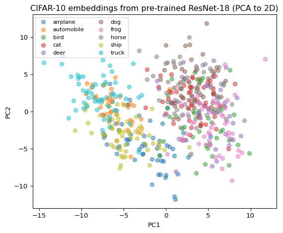
plt.title("CIFAR-10 embeddings from pre-trained ResNet-18 (PCA to 2D)")
plt.legend(fontsize="small", ncol=2)
plt.tight_layout()
plt.show()

Figure: 2D scatter of CIFAR-10 embeddings; many classes form roughly separable clusters.

\(k\)-NN classification in embedding space

from sklearn.neighbors import KNeighborsClassifier
from sklearn.model_selection import train_test_split
from sklearn.metrics import accuracy_score

X_train, X_val, y_train, y_val = train_test_split(
    embeddings, labels, test_size=0.3, random_state=42, stratify=labels
)

knn = KNeighborsClassifier(n_neighbors=5, metric="cosine")
knn.fit(X_train, y_train)
y_pred = knn.predict(X_val)

acc = accuracy_score(y_val, y_pred)
print(f"Validation accuracy with k-NN on ResNet embeddings: {acc:.3f}")

Validation accuracy with k-NN on ResNet embeddings: 0.607

Design choice:

• We use a very simple classifier (\(k\)-NN) to probe the embedding quality.
• If embeddings are good, even a trivial \(k\)-NN can achieve decent accuracy.

Evaluating image embeddings

Metrics & diagnostics:

• Linear probe accuracy:
  • Freeze the embedding model, train a small linear classifier on top.
• \(k\)-NN accuracy:
  • As we just did—very low-overhead sanity check.
• Retrieval metrics:
  • For each query image, retrieve nearest neighbours and inspect:
    • Qualitative: are neighbours “visually / semantically similar”?
    • Quantitative: precision@\(k\), recall@\(k\)
• Visual checks:
  • 2D PCA / t-SNE / UMAP plots
  • Look for class clusters, overlaps, outliers

Remember

• Nice clusters ≠ proof of generalization.
• Overfitting can still occur if embeddings are too specialized to training data.

Summary

🔬 Graph embeddings: intuition

Setting:

• We have a graph \(G = (V, E)\):
  • Nodes: users, products, papers, proteins, …
  • Edges: friendships, co-purchases, citations, interactions

Goal:

• Learn \(f_\text{graph}: V \to \mathbb{R}^d\) so that:
  • Connected / structurally similar nodes have similar embeddings.
  • Useful for downstream tasks:
    • Link prediction
    • Node classification
    • Community detection
    • Recommendation

Examples:

• DeepWalk (Perozzi, Al-Rfou, and Skiena 2014) / node2vec (Grover and Leskovec 2016):
  • Run random walks on the graph.
  • Treat these walks like sentences.
  • Use word2vec-style training on node sequences.
• Graph neural networks (GNNs) (Kipf and Welling 2017):
  • Iteratively aggregate neighbour features.
  • Every layer updates node embeddings.

Evaluation & quality checks (cross-modal)

Common strategies across text, image, graph embeddings:

• Downstream tasks
  • Classification / regression using embeddings as features.
  • Link prediction, recommendation, semantic search.
• Neighbourhood analysis
  • Look at nearest neighbours:
    • Are they semantically / structurally meaningful?
• Clustering quality
  • Cluster embeddings and compare to known groups (if labels exist).
  • Metrics: silhouette score, NMI, ARI, …
• Robustness tests
  • Slightly perturb inputs (augmentations).
  • Check whether neighbours / predictions are stable.

Always ask

What is this embedding space actually good for?
And: On which data distribution and for whose benefit?

Ethics & risks in embeddings

Bias & stereotypes (Caliskan, Bryson, and Narayanan 2017; Buolamwini and Gebru 2018)

• Word embeddings trained on web corpora have been shown to encode:
  • Gender stereotypes (“programmer” near “man”, “nurse” near “woman”)
  • Racial, religious, and cultural biases
• Image embeddings (and their training data) can reflect:
  • Unequal representation across groups
  • Biased labels or annotation practices

Privacy & leakage (Shokri et al. 2017; Song and Raghunathan 2020; Morris et al. 2023)

• Embeddings may leak information about:
  • Sensitive attributes (even if not explicitly included)
  • Membership of individuals in the training set (membership inference attacks)

Mitigations (intro level) (Bolukbasi et al. 2016; Zemel et al. 2013; Chen et al. 2020; Balagopalan et al. 2022)

• Use filtered / curated pre-trained models when possible.
• Perform bias probes:
  • Compare distances to group-related words / images.
• Use embeddings as one signal among many, with human oversight.
• If decisions impact people:
  • Perform fairness analysis on the full system, not just on embeddings.

Quick check

1. MCQ – cosine similarity vs dot product

Suppose \(u\) and \(v\) are embeddings in \(\mathbb{R}^d\).

Which statement is most accurate?

A. Cosine similarity and dot product are always identical.
B. Cosine similarity ignores vector norms, dot product does not.
C. Cosine similarity is only defined in 2D.
D. Dot product is always between −1 and 1, cosine similarity is unbounded.

2. Short conceptual

Why might a k-NN classifier on ResNet embeddings of CIFAR-10 images outperform k-NN directly on raw pixels?

3. Numeric

Two unit-norm embedding vectors have dot product \(0.8\). What is the angle between them (in degrees, approximately)?

4. MCQ – embedding misuse

Which scenario is most clearly an embedding misuse?

A. Using word embeddings as input features for a sentiment classifier.
B. Using image embeddings plus k-NN for image retrieval.
C. Ranking job applicants solely by cosine similarity between their text embeddings and the text embeddings of past successful hires, without any fairness analysis.
D. Visualizing embeddings with t-SNE for exploratory analysis.

References

Balagopalan, Aparna, Haoran Zhang, Kimia Hamidieh, Thomas Hartvigsen, Frank Rudzicz, and Marzyeh Ghassemi. 2022. “The Road to Explainability Is Paved with Bias: Measuring the Fairness of Explanations.” In Proceedings of the 2022 ACM Conference on Fairness, Accountability, and Transparency (FAccT), 1194–1206. ACM.

Bojanowski, Piotr, Edouard Grave, Armand Joulin, and Tomas Mikolov. 2017. “Enriching Word Vectors with Subword Information.” Transactions of the Association for Computational Linguistics 5: 135–46.

Bolukbasi, Tolga, Kai-Wei Chang, James Y. Zou, Venkatesh Saligrama, and Adam T. Kalai. 2016. “Man Is to Computer Programmer as Woman Is to Homemaker? Debiasing Word Embeddings.” In Advances in Neural Information Processing Systems 29 (NeurIPS), 4349–57.

Buolamwini, Joy, and Timnit Gebru. 2018. “Gender Shades: Intersectional Accuracy Disparities in Commercial Gender Classification.” In Proceedings of the Conference on Fairness, Accountability, and Transparency, 81:77–91. Proceedings of Machine Learning Research. PMLR.

Caliskan, Aylin, Joanna J. Bryson, and Arvind Narayanan. 2017. “Semantics Derived Automatically from Language Corpora Contain Human-Like Biases.” Science 356 (6334): 183–86. https://doi.org/10.1126/science.aal4230.

Chen, John, Ian Berlot-Attwell, Xindi Wang, Safwan Hossain, and Frank Rudzicz. 2020. “Exploring Text Specific and Blackbox Fairness Algorithms in Multimodal Clinical NLP.” In Proceedings of the 3rd Clinical Natural Language Processing Workshop, 301–12. Online: Association for Computational Linguistics. https://doi.org/10.18653/v1/2020.clinicalnlp-1.33.

Devlin, Jacob, Ming-Wei Chang, Kenton Lee, and Kristina Toutanova. 2019. “BERT: Pre-Training of Deep Bidirectional Transformers for Language Understanding.” In Proceedings of the 2019 Conference of the North American Chapter of the Association for Computational Linguistics: Human Language Technologies (NAACL-HLT), 4171–86.

Grover, Aditya, and Jure Leskovec. 2016. “Node2vec: Scalable Feature Learning for Networks.” In Proceedings of the 22nd ACM SIGKDD International Conference on Knowledge Discovery and Data Mining, 855–64. ACM.

Kipf, Thomas N., and Max Welling. 2017. “Semi-Supervised Classification with Graph Convolutional Networks.” In Proceedings of the 5th International Conference on Learning Representations.

Manning, Christopher D., Prabhakar Raghavan, and Hinrich Schütze. 2008. Introduction to Information Retrieval. Cambridge University Press.

Mikolov, Tomas, Kai Chen, Greg Corrado, and Jeffrey Dean. 2013. “Efficient Estimation of Word Representations in Vector Space.” In Proceedings of the International Conference on Learning Representations (ICLR), Workshop Track.

Morris, John X., Volodymyr Kuleshov, Vitaly Shmatikov, and Alexander M. Rush. 2023. “Text Embeddings Reveal (Almost) as Much as Text.” In Proceedings of the 2023 Conference on Empirical Methods in Natural Language Processing (EMNLP), 12448–60. Association for Computational Linguistics.

Pennington, Jeffrey, Richard Socher, and Christopher D. Manning. 2014. “GloVe: Global Vectors for Word Representation.” In Proceedings of the 2014 Conference on Empirical Methods in Natural Language Processing (EMNLP), 1532–43.

Perozzi, Bryan, Rami Al-Rfou, and Steven Skiena. 2014. “DeepWalk: Online Learning of Social Representations.” In Proceedings of the 20th ACM SIGKDD International Conference on Knowledge Discovery and Data Mining, 701–10. ACM.

Peters, Matthew E., Mark Neumann, Mohit Iyyer, Matt Gardner, Christopher Clark, Kenton Lee, and Luke Zettlemoyer. 2018. “Deep Contextualized Word Representations.” In Proceedings of the 2018 Conference of the North American Chapter of the Association for Computational Linguistics: Human Language Technologies (NAACL-HLT), 2227–37.

Radford, Alec, Karthik Narasimhan, Tim Salimans, and Ilya Sutskever. 2018. “Improving Language Understanding by Generative Pre-Training.” OpenAI.

Shokri, Reza, Marco Stronati, Congzheng Song, and Vitaly Shmatikov. 2017. “Membership Inference Attacks Against Machine Learning Models.” In 2017 IEEE Symposium on Security and Privacy (SP), 3–18. IEEE. https://doi.org/10.1109/SP.2017.41.

Song, Congzheng, and Ananth Raghunathan. 2020. “Information Leakage in Embedding Models.” In Proceedings of the 2020 ACM SIGSAC Conference on Computer and Communications Security (CCS), 377–90. ACM. https://doi.org/10.1145/3372297.3417270.

Zemel, Richard, Yu Wu, Kevin Swersky, Toniann Pitassi, and Cynthia Dwork. 2013. “Learning Fair Representations.” In Proceedings of the 30th International Conference on Machine Learning (ICML), 28:325–33. Proceedings of Machine Learning Research 3. PMLR.