M40: Principles of Representation Learning

CSCI 3151 — Foundations of Machine Learning

Frank Rudzicz

Learning outcomes

By the end of this module, you should be able to:

Define what a representation is and distinguish it from a model or classifier.
Describe and justify qualitative properties of good representations (e.g., invariance, expressivity, disentanglement, task-alignment).
Explain how different training objectives (supervised vs self-/unsupervised) shape learned representations.
Implement and analyze small experiments that compare raw features vs learned representations, using both tables and visualizations.
Critically evaluate representation plots/embeddings, including ethical and robustness concerns (e.g., leakage, fairness, misleading clusters).

From raw data to representations

Think of our ML pipeline as:

\[ x \in \mathcal{X} \;\xrightarrow{\;\phi\;}\; \boxed{z \in \mathcal{Z}} \;\xrightarrow{\;g\;}\; \hat{y} \in \mathcal{Y} \]

\(x\): raw input (image, text sequence, tabular features, graph, audio…)
\(\phi\): representation function (a.k.a. encoder, feature map, embedding model)
\(z = \phi(x)\): representation (feature vector / embedding)
\(g\): simple predictor / head (e.g. linear classifier, shallow MLP)

Representation learning n.: is the process of training a model so that it maps raw data into a new space of representations (embeddings / feature vectors) that make important tasks (like classification, prediction, retrieval, generation) easier to solve (Bengio, Courville, and Vincent 2013; Goodfellow, Bengio, and Courville 2016).

Representations vs models

In classical ML:
- “Features” = manual, hand-designed transforms of raw inputs
- Model = logistic regression / SVM on those features
In deep learning:
- Representation \(\phi_\theta\) is learned (e.g., CNN trunk), often with many parameters
- Simple heads \(g_w\) sit on top (linear layer, shallow MLP)

We often factor a big model into:

Backbone / encoder (representation)
Head (task-specific readout)

This factorization is what lets us:

Reuse encoders across tasks (transfer learning)
Freeze encoders and train cheap heads
Examine “representation quality”

Good vs bad representations

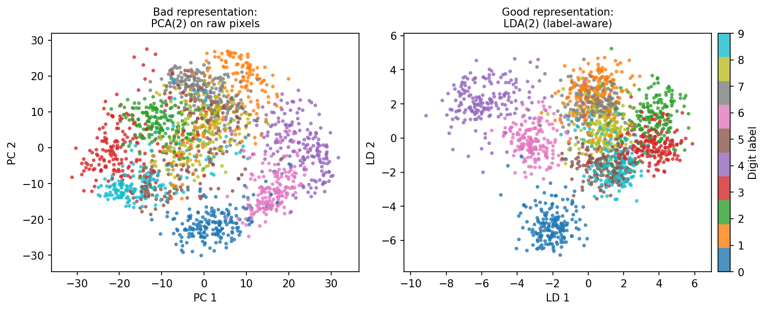
Consider a 2D feature space where each point is an image of a digit, coloured by its true label (0–9):

Bad representation
- All digits are scrambled together
- Distances don’t correlate with semantic similarity
- Any simple classifier has to be highly curved / complex (or just fails)

Good representation
- Each digit class forms a tight cluster
- Clusters are well-separated
- A simple linear boundary can separate classes

We’ll make this intuition precise shortly.

Conceptual scaffold

Key concepts

Representation function
\(\phi: \mathcal{X} \to \mathbb{R}^d\), where \(d\) is the embedding dimension.

Task-aligned representation
\(\phi\) is task-aligned if a simple model on top of \(z = \phi(x)\) performs well.

Invariance
A representation is invariant to a transformation \(T\) (e.g., small translation, rotation, noise) if:

\[ \phi(T(x)) \approx \phi(x) \]

Equivariance
Equivariance means transformations in input space induce predictable transformations in feature space:

\[ \phi(T(x)) \approx A_T \, \phi(x) \]

(e.g., shifting an image shifts feature maps in a CNN).

What makes a good representation?

There is no single universal definition, but common desiderata include:

Expressive enough:
- Can represent the variability needed to solve the tasks of interest.
Task-aligned / linearly separable:
- For classification, classes are (approximately) separable by simple decision surfaces (e.g., linear).
Invariant to nuisance factors:
- Changes that shouldn’t matter for the task (lighting, small rotations, speaking pitch, word order noise) don’t dramatically change the features.
Stable / smooth:
- Small changes in input \(\Rightarrow\) small, meaningful changes in representation (Lipschitz-like behaviour (Scaman and Virmaux 2018)).
Compact or efficient (sometimes):
- Lower dimensionality or sparse representations can help with generalization and interpretability.
Composable:
- Features can be re-used or combined across tasks.

We’ll use these as a checklist when we look at code examples.

❌ Anti-example: “pretty but useless”

Consider a 2D t-SNE plot of patient health records where:

Points form beautiful clusters
A legend claims colours represent disease type
But in reality, colours correspond to hospital ID (where the patient was treated)

Problems:

The representation ended up encoding site-specific artefacts (scanner differences, local practices) instead of biological signal.
Clusters are driven by nuisance factors that may correlate with socio-economic status, race, or insurance status.
A model trained on these representations may perform well on validation data from the same hospitals but fail badly — and unfairly — elsewhere.

This is a bad representation for disease risk: it violates task alignment and bakes in spurious correlations.

Math lens

Representations and linear separability

For a \(K\)-class classification problem:

Suppose the representation function \(\phi\) maps each input \(x\) to \(z = \phi(x) \in \mathbb{R}^d\).
A linear classifier in representation space might have the form:

\[ \hat{y} = \arg\max_{k \in \{1,\dots,K\}} \left( w_k^\top z + b_k \right) \]

If such a classifier achieves low error, we say the representation is approximately linearly separable for this task.

Why do we like linear separability?

Training linear models is:
- Convex (for many losses) → predictable optimization
- Data-efficient relative to huge nonlinear heads
It suggests \(\phi\) has already done the heavy “untangling” of the data manifold.

Information vs simplicity

Let \(x\) be inputs, \(y\) labels, \(z = \phi(x)\) representations.

Two desirable properties (often in tension):

Task information preserved
\[ I(z; y) \quad \text{large (mutual information)} \] so that representations retain predictive signal about labels.
Nuisance compression
\[ I(z; u) \quad \text{small} \] where \(u\) encodes nuisance factors (lighting, site, identity if we care about anonymity, etc.)

We rarely compute these mutual informations exactly in practice, but this information-bottleneck picture is a useful mental model for what “good” representations are trying to achieve.

How objectives shape representations

Consider a parametric encoder \(\phi_\theta\) and a simple linear head \(g_w\).

Different training objectives push \(\phi_\theta\) in different directions:

Supervised classification objective
\[ \min_{\theta, w} \; \mathbb{E}_{(x,y)}\big[ \ell(g_w(\phi_\theta(x)), y) \big] \] Encourages representations where examples of the same class cluster together and are separable from other classes.
Autoencoder / reconstruction objective (Vincent et al. 2008)
\[ \min_{\theta, \psi} \; \mathbb{E}_{x}\big[ \| x - \tilde{x} \|^2 \big], \quad \tilde{x} = \text{dec}_\psi(\phi_\theta(x)) \] where \(\text{dec}_\psi\) is a decoder that maps a representation \(z\) back into data space, producing a reconstruction \(\hat{x}\).
Encourages information-preserving (but not necessarily task-aligned) representations.
Contrastive objective (very simplified) (Chen et al. 2020)
\[ \min_{\theta} \; \mathbb{E}\big[ \ell_{\text{contrastive}}(\phi_\theta(x), \phi_\theta(x^+), \{\phi_\theta(x^-)\}) \big] \] Encourages representations where augmentations of the same input map close together, and different inputs map far apart.

We’ll see echoes of these when we connect to self-supervised methods later in the course.

Worked example 1: Digits

Setup

Goal: compare a “classical” compressed representation (PCA) to raw pixels for digit classification.

Dataset:

sklearn.datasets.load_digits()
~1800 grayscale \(8 \times 8\) digit images (0–9)
Each image → 64-dimensional pixel vector

Steps:

Train logistic regression on standardized raw pixels.
Train logistic regression on PCA-compressed features.
Compare test accuracy and visualize 2D embeddings.

Code: data & baseline

Code

import numpy as np
from sklearn.datasets import load_digits
from sklearn.model_selection import train_test_split
from sklearn.preprocessing import StandardScaler
from sklearn.linear_model import LogisticRegression
from sklearn.pipeline import Pipeline
from sklearn.metrics import accuracy_score, classification_report

# 1. Load data
digits = load_digits()
X, y = digits.data, digits.target  # X: (n_samples, 64)

# 2. Train/test split
X_train, X_test, y_train, y_test = train_test_split(
    X, y, test_size=0.3, random_state=42, stratify=y
)

# 3. Baseline: logistic regression on raw pixels
pipe_raw = Pipeline([
    ("scaler", StandardScaler()),
    ("logreg", LogisticRegression(max_iter=1000, multi_class="multinomial"))
])

pipe_raw.fit(X_train, y_train)
y_pred_raw = pipe_raw.predict(X_test)
acc_raw = accuracy_score(y_test, y_pred_raw)

print(f"Test accuracy (raw pixels): {acc_raw:.3f}")
print(classification_report(y_test, y_pred_raw))

Test accuracy (raw pixels): 0.981
              precision    recall  f1-score   support

           0       1.00      1.00      1.00        54
           1       0.95      0.95      0.95        55
           2       1.00      1.00      1.00        53
           3       1.00      1.00      1.00        55
           4       0.98      0.98      0.98        54
           5       1.00      0.98      0.99        55
           6       1.00      0.98      0.99        54
           7       1.00      1.00      1.00        54
           8       0.91      0.94      0.92        52
           9       0.98      0.98      0.98        54

    accuracy                           0.98       540
   macro avg       0.98      0.98      0.98       540
weighted avg       0.98      0.98      0.98       540

Code: PCA representation

Code

from sklearn.decomposition import PCA
import pandas as pd

# 4. Representation: PCA to 32 dimensions, then logistic regression
pipe_pca = Pipeline([
    ("scaler", StandardScaler()),
    ("pca", PCA(n_components=32, random_state=42)),
    ("logreg", LogisticRegression(max_iter=1000, multi_class="multinomial"))
])

pipe_pca.fit(X_train, y_train)
y_pred_pca = pipe_pca.predict(X_test)
acc_pca = accuracy_score(y_test, y_pred_pca)

# 5. Put results in a small table
results = pd.DataFrame([
    {"Representation": "Raw pixels", "Dim": X.shape[1], "Test accuracy": acc_raw},
    {"Representation": "PCA(32)",   "Dim": 32,          "Test accuracy": acc_pca},
])

results

	Representation	Dim	Test accuracy
0	Raw pixels	64	0.981481
1	PCA(32)	32	0.951852

Tip

Some courses or tutorials act as though every intervention will help.

It’s important to dissipate that fiction, but also be aware of nuances.

2D visualization

Code

import matplotlib.pyplot as plt

# Fit PCA(2) on *train* data only for visualization
pca2 = PCA(n_components=2, random_state=42)
X_train_scaled = StandardScaler().fit_transform(X_train)
X_train_2d = pca2.fit_transform(X_train_scaled)

plt.figure(figsize=(6, 5))
scatter = plt.scatter(
    X_train_2d[:, 0], X_train_2d[:, 1],
    c=y_train, s=12, alpha=0.8
)
plt.xlabel("PC 1")
plt.ylabel("PC 2")
plt.title("Digits: PCA(2) representation coloured by true digit")
plt.colorbar(scatter, ticks=range(10), label="Digit")
plt.tight_layout()
plt.show()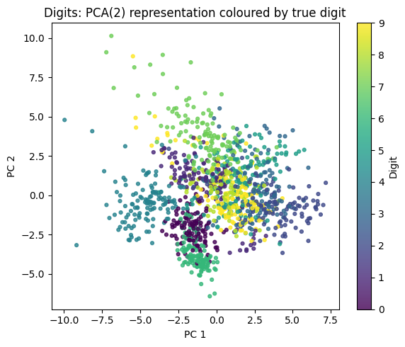

✏️ Check

Do classes form roughly separable clusters?
Are some digits (e.g., 4 & 9) still overlapping?
This tells us how “good” PCA is as a representation for this supervised task.

Discussion

Using our checklist:

Expressive: PCA(32) usually retains most variance → good coverage of data manifold.
Task-aligned:
- If accuracy with PCA(32) is close to or better than raw pixels, PCA has retained most of the label-relevant information while smoothing noise.
Invariant / robust:
- PCA tends to denoise small pixel fluctuations but is not as smart as a CNN about geometric invariances.
Compact:
- 64 → 32 dimensions: cheaper models, potentially less overfitting for deployment.

Caveats

PCA is unsupervised and linear:
- It may preserve directions of high variance that are irrelevant (or even harmful) for classification.
For more complex image structure (e.g., CIFAR-10), we often need nonlinear representations.

Worked example 2: CIFAR-10

Setup (CIFAR-10)

Goal: compare a cheap classifier on:

Raw RGB pixel vectors (flattened images)
Features from the penultimate layer of a small CNN

Dataset:

🔗 CIFAR-10:
- 32x32 colour images, 10 classes
- We’ll sub-sample ~5000 training images for speed in a teaching demo

💡 Idea:

Train a small CNN (yes, we’re getting ahead of ourselves) for a few epochs → get intermediate features.
Freeze the CNN and train a linear classifier on top of the features.
Compare to a linear classifier on flattened pixels.

Data & CNN encoder

Code

import torch
from torch import nn, optim
from torch.utils.data import DataLoader, Subset
from torchvision import datasets, transforms

# 1. Transforms & dataset (simple normalization)
transform = transforms.Compose([
    transforms.ToTensor(),
    transforms.Normalize(mean=[0.5, 0.5, 0.5],
                         std=[0.5, 0.5, 0.5])
])

train_dataset = datasets.CIFAR10(
    root="data", train=True, download=True, transform=transform
)
test_dataset = datasets.CIFAR10(
    root="data", train=False, download=True, transform=transform
)

# Subsample train set for speed
subset_indices = torch.randperm(len(train_dataset))[:5000]
train_subset = Subset(train_dataset, subset_indices)

train_loader = DataLoader(train_subset, batch_size=64, shuffle=True)
test_loader = DataLoader(test_dataset, batch_size=256, shuffle=False)

Small CNN & training

Code

class SmallCNN(nn.Module):
    def __init__(self, feature_dim=256, num_classes=10):
        super().__init__()
        self.features = nn.Sequential(
            nn.Conv2d(3, 32, kernel_size=3, padding=1),
            nn.ReLU(),
            nn.MaxPool2d(2),   # 16x16
            nn.Conv2d(32, 64, kernel_size=3, padding=1),
            nn.ReLU(),
            nn.MaxPool2d(2),   # 8x8
        )
        self.flatten = nn.Flatten()
        self.fc = nn.Sequential(
            nn.Linear(64 * 8 * 8, feature_dim),
            nn.ReLU()
        )
        self.classifier = nn.Linear(feature_dim, num_classes)

    def forward(self, x, return_features=False):
        h = self.features(x)
        h = self.flatten(h)
        z = self.fc(h)              # representation
        logits = self.classifier(z) # head
        if return_features:
            return logits, z
        return logits

device = torch.device("cuda" if torch.cuda.is_available() else "cpu")
model = SmallCNN().to(device)

criterion = nn.CrossEntropyLoss()
optimizer = optim.Adam(model.parameters(), lr=1e-3)

Train CNN (briefly)

Code

def train_epoch(model, loader, optimizer, device):
    model.train()
    running_loss, running_correct, total = 0.0, 0, 0
    for x, y in loader:
        x, y = x.to(device), y.to(device)
        optimizer.zero_grad()
        logits = model(x)
        loss = criterion(logits, y)
        loss.backward()
        optimizer.step()

        running_loss += loss.item() * x.size(0)
        preds = logits.argmax(dim=1)
        running_correct += (preds == y).sum().item()
        total += x.size(0)

    return running_loss / total, running_correct / total

for epoch in range(5):  # a few epochs for demonstration
    loss, acc = train_epoch(model, train_loader, optimizer, device)
    print(f"Epoch {epoch+1}: loss={loss:.4f}, train_acc={acc:.3f}")

Epoch 1: loss=1.8534, train_acc=0.324
Epoch 2: loss=1.4503, train_acc=0.481
Epoch 3: loss=1.2750, train_acc=0.545
Epoch 4: loss=1.1245, train_acc=0.599
Epoch 5: loss=0.9804, train_acc=0.648

Note

In practice, you’d also track validation accuracy, but here our main goal is to learn a useful feature extractor, not to fully tune performance.

Extract representations

We take the CNN trained on CIFAR-10, chop off the final classifier, and run images through it to get \(d\)-dimensional feature vectors from the penultimate layer.
We treat those vectors as learned representations and can then train a simple linear classifier (or visualize them with PCA/t-SNE) on top.

Code

import numpy as np

def extract_representations(model, loader, device):
    model.eval()
    features_list, labels_list = [], []
    with torch.no_grad():
        for x, y in loader:
            x = x.to(device)
            logits, z = model(x, return_features=True)
            features_list.append(z.cpu().numpy())
            labels_list.append(y.numpy())
    return np.concatenate(features_list, axis=0), np.concatenate(labels_list, axis=0)

# 1. Extract train/test features
Z_train, y_train = extract_representations(model, train_loader, device)
Z_test,  y_test  = extract_representations(model, test_loader, device)

print("Train features shape:", Z_train.shape)  # e.g., (5000, 256)
print("Test features shape:", Z_test.shape)

Train features shape: (5000, 256)
Test features shape: (10000, 256)

Linear classifiers (pixels vs features)

Code

from sklearn.linear_model import LogisticRegression
from sklearn.metrics import accuracy_score
from tqdm import tqdm

# 2. Baseline: linear classifier on raw flattened pixels

# Build flattened pixel arrays for the *same* subsets
def collect_flat_pixels(loader):
    X_list, y_list = [], []
    for x, y in loader:
        # x: (B, C, H, W)
        X_list.append(x.view(x.size(0), -1).numpy())
        y_list.append(y.numpy())
    return np.concatenate(X_list, axis=0), np.concatenate(y_list, axis=0)

X_train_flat, y_train_flat = collect_flat_pixels(train_loader)
X_test_flat,  y_test_flat  = collect_flat_pixels(test_loader)

logreg_pixels = LogisticRegression(
    max_iter=200, multi_class="multinomial", n_jobs=-1
)
logreg_pixels.fit(X_train_flat, y_train_flat)
y_pred_pixels = logreg_pixels.predict(X_test_flat)
acc_pixels = accuracy_score(y_test_flat, y_pred_pixels)

# 3. Linear classifier on CNN representations
logreg_repr = LogisticRegression(
    max_iter=200, multi_class="multinomial", n_jobs=-1
)
logreg_repr.fit(Z_train, y_train)
y_pred_repr = logreg_repr.predict(Z_test)
acc_repr = accuracy_score(y_test, y_pred_repr)

print("Test accuracy (linear on pixels):", acc_pixels)
print("Test accuracy (linear on CNN features):", acc_repr)

Test accuracy (linear on pixels): 0.28
Test accuracy (linear on CNN features): 0.5499

Results

Code

import pandas as pd
from sklearn.decomposition import PCA
import matplotlib.pyplot as plt

results = pd.DataFrame([
    {"Representation": "Flattened pixels", "Dim": X_train_flat.shape[1],
     "Test accuracy": acc_pixels},
    {"Representation": "CNN features",     "Dim": Z_train.shape[1],
     "Test accuracy": acc_repr},
])

results

	Representation	Dim	Test accuracy
0	Flattened pixels	3072	0.2800
1	CNN features	256	0.5499

Code

# 2D PCA of CNN features for visualization
pca2 = PCA(n_components=2, random_state=42)
Z_test_2d = pca2.fit_transform(Z_test)

plt.figure(figsize=(6, 5))
scatter = plt.scatter(
    Z_test_2d[:, 0], Z_test_2d[:, 1],
    c=y_test, s=8, alpha=0.7
)
plt.xlabel("PC 1")
plt.ylabel("PC 2")
plt.title("CIFAR-10: PCA(2) of CNN representations")
plt.colorbar(scatter, ticks=range(10), label="Class")
plt.tight_layout()
plt.show()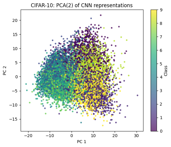

What we typically see

Linear on raw pixels: modest accuracy, struggles due to high-dimensional, poorly structured features.
Linear on CNN features: noticeably better accuracy — the encoder has learned a more task-aligned representation.

Representation principles in action

Using our checklist:

Expressive: CNN features live in a 256-dim space with nonlinear filters → able to capture complex patterns.
Task-aligned: Linear classifier on features outperforms linear classifier on raw pixels.
Invariance / equivariance:
- Convolutions + pooling → some translation invariance, local pattern detection.
Reusability:
- Same CNN encoder could be adapted for related tasks (e.g., CIFAR-100 subset, coarse category grouping) by swapping the head.

🔑 Key lesson

A “good” representation is one where simple downstream models work well and where geometry aligns with task semantics.

Summary

Evaluation: for what are we optimizing?

We need to align:

Objective used to learn \(\phi\) (e.g., supervised cross-entropy, contrastive loss, reconstruction loss)
Metric used to evaluate downstream tasks (e.g., accuracy, F1, calibration error)
Representation diagnostics (e.g., linear probe accuracy, clustering quality, embedding plots)

Example diagnostics:

Linear probe:
- Freeze \(\phi\), train a linear classifier → how well does it do?
k-NN accuracy in representation space:
- Close points should often share labels.
Visual sanity checks:
- PCA/t-SNE/UMAP of representations coloured by label.
- But beware over-interpreting pretty pictures!

Metrics for representation quality

Some practical proxies (beyond loss):

Downstream accuracy of simple models (e.g., LR on frozen features).
Sample efficiency:
- How much labelled data do we need to reach a target accuracy with a simple head?
Clustering metrics (unsupervised settings):
- Silhouette score, NMI/ARI vs ground truth clusters (when available).
Robustness:
- Performance under distribution shifts (e.g., mild corruptions, sub-population shifts).

Important

These are task-dependent; there is no single scalar “representation goodness score” that works for everything.

🔬 Real-world systems & research threads

A few examples where representation learning is central:

Image–text models (e.g., CLIP-like systems) (Radford et al. 2021):
- Learn joint embeddings for images and captions → zero-shot classification.
Large language models (Devlin et al. 2019; Brown et al. 2020):
- Token embeddings and contextual representations are the backbone for all downstream tasks.
Graph embeddings (Grover and Leskovec 2016):
- Nodes in a graph represented as vectors → used for link prediction, recommendation, fraud detection.

Research questions you could pursue later:

How do we measure representation quality rigorously?
(e.g., representational similarity / CKA-style metrics (Kornblith et al. 2019))
How can we enforce fairness and privacy at the level of representations?
(fair representations and DP training (Zemel et al. 2013; Abadi et al. 2016))
Can we design objectives that produce universally useful embeddings across many tasks?
(large-scale pretraining and multimodal models (Radford et al. 2021; Brown et al. 2020))

Quick checks

Which of the following best describes a task-aligned representation?

A. One that perfectly reconstructs the input.
B. One where a simple model achieves high performance on the target task.
C. One that minimizes the mutual information \(I(z; x)\).
D. One that uses as few dimensions as possible.
In Example 2 (CIFAR-10), why does a linear classifier on CNN features typically outperform a linear classifier on flattened pixels?

A. CNN features have more dimensions than pixels.
B. CNN features are explicitly optimized to be linearly separable for the training labels.
C. Linear classifiers cannot operate directly on pixel inputs.
D. The CNN features are random and thus more robust.
Which of the following is not a common desideratum for a good representation?

A. Invariance to nuisance transformations.
B. High mutual information with irrelevant environment variables.
C. Smoothness: small input changes → small representation changes.
D. Task alignment for simple downstream heads.
Suppose you train an autoencoder on images and use its latent code as a representation for classification. Which concern is most appropriate?

A. Latent codes will always be linearly separable for any label.
B. Reconstruction objectives may preserve details irrelevant or harmful for the classification task.
C. Autoencoders never leak sensitive attributes.
D. Autoencoders cannot be trained on images with more than 64x64 pixels.

References

Abadi, Martin, Andy Chu, Ian Goodfellow, H. Brendan McMahan, Ilya Mironov, Kunal Talwar, and Li Zhang. 2016. “Deep Learning with Differential Privacy.” In Proceedings of the 2016 ACM SIGSAC Conference on Computer and Communications Security, 308–18.

Bengio, Yoshua, Aaron Courville, and Pascal Vincent. 2013. “Representation Learning: A Review and New Perspectives.” IEEE Transactions on Pattern Analysis and Machine Intelligence 35 (8): 1798–828. https://doi.org/10.1109/TPAMI.2013.50.

Brown, Tom B., Benjamin Mann, Nick Ryder, Melanie Subbiah, Jared Kaplan, Prafulla Dhariwal, Arvind Neelakantan, et al. 2020. “Language Models Are Few-Shot Learners.” In Advances in Neural Information Processing Systems, 33:1877–1901.

Chen, Ting, Simon Kornblith, Mohammad Norouzi, and Geoffrey Hinton. 2020. “A Simple Framework for Contrastive Learning of Visual Representations.” In Proceedings of the 37th International Conference on Machine Learning (ICML).

Devlin, Jacob, Ming-Wei Chang, Kenton Lee, and Kristina Toutanova. 2019. “BERT: Pre-Training of Deep Bidirectional Transformers for Language Understanding.” In Proceedings of the 2019 Conference of the North American Chapter of the Association for Computational Linguistics: Human Language Technologies (NAACL-HLT), 4171–86.

Goodfellow, Ian, Yoshua Bengio, and Aaron Courville. 2016. Deep Learning. MIT Press. http://www.deeplearningbook.org.

Grover, Aditya, and Jure Leskovec. 2016. “Node2vec: Scalable Feature Learning for Networks.” In Proceedings of the 22nd ACM SIGKDD International Conference on Knowledge Discovery and Data Mining, 855–64. ACM.

Kornblith, Simon, Mohammad Norouzi, Honglak Lee, and Geoffrey Hinton. 2019. “Similarity of Neural Network Representations Revisited.” In Proceedings of the 36th International Conference on Machine Learning, 97:3519–29. Proceedings of Machine Learning Research.

Radford, Alec, Jong Wook Kim, Chris Hallacy, Aditya Ramesh, Gabriel Goh, Sandhini Agarwal, Girish Sastry, et al. 2021. “Learning Transferable Visual Models from Natural Language Supervision.” In Proceedings of the 38th International Conference on Machine Learning, 139:8748–63. PMLR.

Scaman, Kevin, and Aladin Virmaux. 2018. “Lipschitz Regularity of Deep Neural Networks: Analysis and Efficient Estimation.” In Advances in Neural Information Processing Systems. Vol. 31. https://arxiv.org/abs/1805.10965.

Vincent, Pascal, Hugo Larochelle, Yoshua Bengio, and Pierre-Antoine Manzagol. 2008. “Extracting and Composing Robust Features with Denoising Autoencoders.” In Proceedings of the 25th International Conference on Machine Learning (ICML).

Zemel, Rich, Yu Wu, Kevin Swersky, Toniann Pitassi, and Cynthia Dwork. 2013. “Learning Fair Representations.” In Proceedings of the 30th International Conference on Machine Learning, 325–33.