M38: Dropout, Batch Normalization, and Training Tricks

CSCI 3151 — Foundations of Machine Learning

Frank Rudzicz

Table of contents

• Conceptual scaffold
• Worked example 1
• Batch Normalization
• Worked example 2
• Summary

Learning Outcomes

By the end of this module, you should be able to:

1. Explain the intuition behind dropout as a regularizer and approximate ensemble method.
2. Write down and implement the core equations for batch normalization and interpret its parameters.
3. Compare training and validation curves with and without dropout / batchnorm to diagnose overfitting and training instability.
4. Design and justify simple training tricks (e.g., early stopping, gradient clipping, learning-rate schedules) for a given deep network.
5. Recognize failure modes when these tricks are misused (e.g., too much dropout, wrong BatchNorm configuration, over-tuned schedules).

The New Question

We can now train deep networks, using modern frameworks.
How do we make them generalize well and train stably in practice?

• Real-world training often hits:
  • Overfitting on small-ish datasets
  • Unstable or painfully slow optimization
  • Sensitivity to learning rate and initialization
• Practitioners reach for:
  • Dropout
  • Batch normalization
  • A grab-bag of small training tricks

Conceptual scaffold

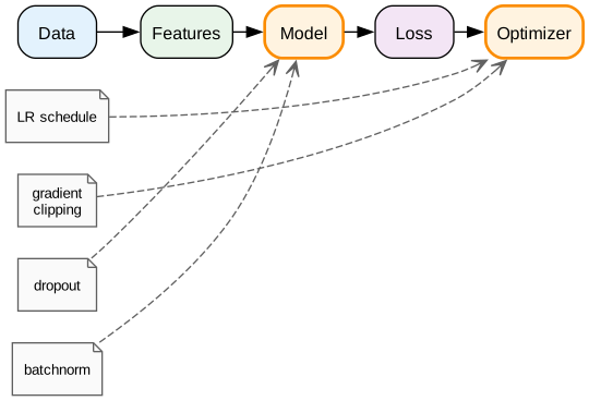
Knobs We Can Turn

Think of four big levers:

1. Data & labels
   • More data, better labels, augmentation
2. Model & representation
   • Architecture, depth, width, feature learning
3. Objective & evaluation
   • Loss functions, metrics, splits, cross-validation
4. Optimization & regularization
   • Learning rates, weight decay, early stopping
   • 👉Dropout, batchnorm, and related tricks (this module 👀)

Dropout: Intuition

💡 Idea (Srivastava et al. 2014; Gal and Ghahramani 2016):
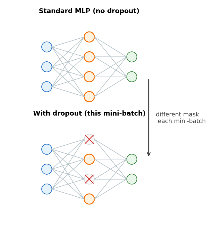
At training time, randomly “drop” (set to 0) some hidden units.

• Prevents co-adaptation:
  • Individual units can’t rely on a specific other unit always being present.
• Acts like training a large ensemble of thinned networks and averaging them at test time.
• Behaves as a kind of noise injection on hidden activations, which:
  • Encourages robustness
  • Acts as implicit regularization (similar in spirit to weight decay, e.g., L2)

Dropout: Simple Math View

Consider a hidden layer activation vector \(h \in \mathbb{R}^d\).

• Training time:
  • Sample a dropout mask: \[ m_i \sim \text{Bernoulli}(p), \quad i = 1,\dots,d \]
  • Most modern libraries implement the “inverted” variant of dropout, where activations are at training time so that no scaling is needed at test time (see e.g. PyTorch’s 🔗 nn.Dropout): \[ \tilde{h}_i = \frac{m_i}{p} \, h_i \]
  • So: \[ \mathbb{E}[\tilde{h}_i] = h_i \]
• Test time:
  • Use the full activation: \[ \tilde{h}_i = h_i \]
  • Because scaling was done during training.
• 🔑 Key hyperparameter:
  • keep probability \(p\) (or equivalently drop probability \(1 - p\)).

Dropout in PyTorch

import torch
import torch.nn as nn
import torch.nn.functional as F

class DropoutMLP(nn.Module):
    def __init__(self, input_dim, hidden_dim, num_classes, p_drop=0.5):
        super().__init__()
        self.fc1 = nn.Linear(input_dim, hidden_dim)
        self.dropout1 = nn.Dropout(p=p_drop)
        self.fc2 = nn.Linear(hidden_dim, hidden_dim)
        self.dropout2 = nn.Dropout(p=p_drop)
        self.out = nn.Linear(hidden_dim, num_classes)

    def forward(self, x):
        # x: (batch_size, input_dim)
        x = F.relu(self.fc1(x))
        x = self.dropout1(x)       # only active in model.train() mode
        x = F.relu(self.fc2(x))
        x = self.dropout2(x)
        return self.out(x)

• nn.Dropout automatically:
  • Uses inverted dropout at training time
  • Disables dropping at evaluation time

Worked example 1

Dropout on Two Moons

Goal: see how dropout changes generalization on a small, overparameterized model.

import numpy as np
from sklearn.datasets import make_moons
from sklearn.model_selection import train_test_split
from sklearn.preprocessing import StandardScaler
import torch
from torch.utils.data import TensorDataset, DataLoader
import matplotlib.pyplot as plt

# Generate data
X, y = make_moons(n_samples=2000, noise=0.25, random_state=3151)
X_train, X_val, y_train, y_val = train_test_split(
    X, y, test_size=0.3, stratify=y, random_state=0
)

scaler = StandardScaler().fit(X_train)
X_train = scaler.transform(X_train)
X_val = scaler.transform(X_val)

X_train_t = torch.tensor(X_train, dtype=torch.float32)
y_train_t = torch.tensor(y_train, dtype=torch.long)
X_val_t   = torch.tensor(X_val, dtype=torch.float32)
y_val_t   = torch.tensor(y_val, dtype=torch.long)

train_ds = TensorDataset(X_train_t, y_train_t)
val_ds   = TensorDataset(X_val_t, y_val_t)

train_loader = DataLoader(train_ds, batch_size=64, shuffle=True)
val_loader   = DataLoader(val_ds, batch_size=256)

Training Loop 🔁

def train_model(model, train_loader, val_loader, epochs=50, lr=1e-2, device="cpu"):
    model.to(device)
    opt = torch.optim.Adam(model.parameters(), lr=lr)
    criterion = nn.CrossEntropyLoss()

    history = {"train_loss": [], "val_loss": [], "train_acc": [], "val_acc": []}

    for epoch in range(epochs):
        model.train()
        running_loss, correct, total = 0.0, 0, 0
        for xb, yb in train_loader:
            xb, yb = xb.to(device), yb.to(device)
            opt.zero_grad()
            logits = model(xb)
            loss = criterion(logits, yb)
            loss.backward()
            opt.step()

            running_loss += loss.item() * xb.size(0)
            preds = logits.argmax(dim=1)
            correct += (preds == yb).sum().item()
            total += xb.size(0)

        train_loss = running_loss / total
        train_acc = correct / total

        # Validation
        model.eval()
        val_loss, correct, total = 0.0, 0, 0
        with torch.no_grad():
            for xb, yb in val_loader:
                xb, yb = xb.to(device), yb.to(device)
                logits = model(xb)
                loss = criterion(logits, yb)
                val_loss += loss.item() * xb.size(0)
                preds = logits.argmax(dim=1)
                correct += (preds == yb).sum().item()
                total += xb.size(0)
        val_loss /= total
        val_acc = correct / total

        history["train_loss"].append(train_loss)
        history["val_loss"].append(val_loss)
        history["train_acc"].append(train_acc)
        history["val_acc"].append(val_acc)
    return history

Ablation: With & Without Dropout

Ablation n.: systematically removing or disabling a component of a model (or training recipe) to see how much it actually matters for performance.

# Without dropout
plain_mlp = DropoutMLP(input_dim=2, hidden_dim=64, num_classes=2, p_drop=0.0)
hist_plain = train_model(plain_mlp, train_loader, val_loader, epochs=80)

# With dropout
drop_mlp = DropoutMLP(input_dim=2, hidden_dim=64, num_classes=2, p_drop=0.5)
hist_drop = train_model(drop_mlp, train_loader, val_loader, epochs=80)

# Make a small summary table
import pandas as pd

summary = pd.DataFrame({
    "model": ["plain", "dropout"],
    "final_train_acc": [
        hist_plain["train_acc"][-1],
        hist_drop["train_acc"][-1],
    ],
    "final_val_acc": [
        hist_plain["val_acc"][-1],
        hist_drop["val_acc"][-1],
    ]
})
summary

	model	final_train_acc	final_val_acc
0	plain	0.945000	0.936667
1	dropout	0.940714	0.930000

• Expectation:
  • Plain model: very high training accuracy, slightly worse validation accuracy.
  • Dropout model: slightly lower training accuracy, often better validation accuracy.

Plotting the Curves

plt.figure(figsize=(6, 4))
plt.plot(hist_plain["train_acc"], label="train (plain)")
plt.plot(hist_plain["val_acc"], label="val (plain)", linestyle="--")
plt.plot(hist_drop["train_acc"], label="train (dropout)")
plt.plot(hist_drop["val_acc"], label="val (dropout)", linestyle="--")
plt.xlabel("Epoch")
plt.ylabel("Accuracy")
plt.title("Two Moons: Dropout vs Plain MLP")
plt.legend()
plt.tight_layout()
plt.show()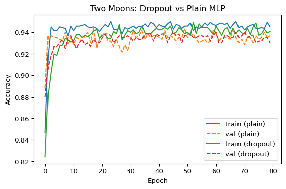

Takeaways

• Dropout tends to:
  • Slow down overfitting
  • Improve validation accuracy especially when:
    • Model capacity is high
    • Dataset is small / moderately noisy

❌ When Dropout Can Go Wrong

• Very small models or tiny datasets:
  • High dropout → underfitting (both training & validation accuracy low)
• Using dropout on:
  • Batchnorm-normalized layers and aggressively using weight decay
  • May “over-regularize” and hurt performance
• Sequence models & certain architectures:
  • Naive dropout at every time step can harm long-range dependencies
  • Specialized variants (e.g., variational dropout) are preferred

👍 Short rule of thumb

If training accuracy never gets high, and you’re using dropout, consider lowering dropout or removing it.

Batch Normalization

Batch Normalization: Intuition

Key problem:
Deep nets are sensitive to the scale / distribution of activations.

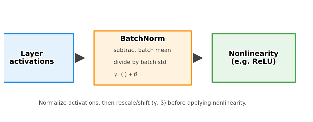
BatchNorm solution (Ioffe and Szegedy 2015):

• For each mini-batch and channel:
  • Normalize activations to have mean ≈ 0 and variance ≈ 1
• Then learn a scale and shift to restore flexibility
• Benefits:
  • Smoother optimization surface
  • Allows higher learning rates
  • Reduces sensitivity to initialization
  • Often improves generalization

Batch Normalization: Equations

Given activations \(x_1, \dots, x_m\) in a mini-batch (for one feature channel):

• Compute batch statistics: \[ \mu_B = \frac{1}{m} \sum_{i=1}^m x_i, \qquad \sigma_B^2 = \frac{1}{m} \sum_{i=1}^m (x_i - \mu_B)^2 \]
• Normalize: \[ \hat{x}_i = \frac{x_i - \mu_B}{\sqrt{\sigma_B^2 + \epsilon}} \]
• Scale and shift: \[ y_i = \gamma \hat{x}_i + \beta \] where \(\gamma, \beta\) are learned parameters.

Training vs inference

• Training: uses per-batch \(\mu_B, \sigma_B^2\)
• Inference: uses running averages estimated during training

BatchNorm in PyTorch

Example for a fully-connected layer:

class DeepPlainMLP(nn.Module):
    def __init__(self, input_dim=2, hidden_dim=128, num_classes=2):
        super().__init__()
        self.fc1 = nn.Linear(input_dim, hidden_dim)
        self.fc2 = nn.Linear(hidden_dim, hidden_dim)
        self.fc3 = nn.Linear(hidden_dim, hidden_dim)
        self.fc4 = nn.Linear(hidden_dim, hidden_dim)
        self.fc5 = nn.Linear(hidden_dim, hidden_dim)
        self.out = nn.Linear(hidden_dim, num_classes)

    def forward(self, x):
        x = F.relu(self.fc1(x))
        x = F.relu(self.fc2(x))
        x = F.relu(self.fc3(x))
        x = F.relu(self.fc4(x))
        x = F.relu(self.fc5(x))
        return self.out(x)


class DeepBNMLP(nn.Module):
    def __init__(self, input_dim=2, hidden_dim=128, num_classes=2):
        super().__init__()
        self.fc1 = nn.Linear(input_dim, hidden_dim)
        self.bn1 = nn.BatchNorm1d(hidden_dim)
        self.fc2 = nn.Linear(hidden_dim, hidden_dim)
        self.bn2 = nn.BatchNorm1d(hidden_dim)
        self.fc3 = nn.Linear(hidden_dim, hidden_dim)
        self.bn3 = nn.BatchNorm1d(hidden_dim)
        self.fc4 = nn.Linear(hidden_dim, hidden_dim)
        self.bn4 = nn.BatchNorm1d(hidden_dim)
        self.fc5 = nn.Linear(hidden_dim, hidden_dim)
        self.bn5 = nn.BatchNorm1d(hidden_dim)
        self.out = nn.Linear(hidden_dim, num_classes)

    def forward(self, x):
        x = F.relu(self.bn1(self.fc1(x)))
        x = F.relu(self.bn2(self.fc2(x)))
        x = F.relu(self.bn3(self.fc3(x)))
        x = F.relu(self.bn4(self.fc4(x)))
        x = F.relu(self.bn5(self.fc5(x)))
        return self.out(x)

• For images, use nn.BatchNorm2d(channels) after convolution layers.
• For sequences, nn.BatchNorm1d + careful reshaping, or alternatives like LayerNorm.

Worked example 2

BatchNorm vs No BatchNorm

We’ll use the same two-moons data but a deeper network and a slightly higher learning rate to expose instability.

# ----------------- training with SGD (larger LR) ---------------------------
def train_model_sgd(model, train_loader, val_loader, epochs=80, lr=0.5, device="cpu"):
    model.to(device)
    opt = torch.optim.SGD(model.parameters(), lr=lr)
    criterion = nn.CrossEntropyLoss()

    history = {"train_loss": [], "val_loss": []}

    for epoch in range(epochs):
        model.train()
        running_loss, total = 0.0, 0
        for xb, yb in train_loader:
            xb, yb = xb.to(device), yb.to(device)
            opt.zero_grad()
            logits = model(xb)
            loss = criterion(logits, yb)
            loss.backward()
            opt.step()

            running_loss += loss.item() * xb.size(0)
            total += xb.size(0)

        train_loss = running_loss / total

        # validation
        model.eval()
        val_loss, total = 0.0, 0
        with torch.no_grad():
            for xb, yb in val_loader:
                xb, yb = xb.to(device), yb.to(device)
                logits = model(xb)
                loss = criterion(logits, yb)
                val_loss += loss.item() * xb.size(0)
                total += xb.size(0)
        val_loss /= total

        history["train_loss"].append(train_loss)
        history["val_loss"].append(val_loss)

    return history

X, y = make_moons(n_samples=4000, noise=0.25, random_state=3151)
X_train, X_val, y_train, y_val = train_test_split(
    X, y, test_size=0.3, stratify=y, random_state=0
)

X_train_t = torch.tensor(X_train, dtype=torch.float32)
y_train_t = torch.tensor(y_train, dtype=torch.long)
X_val_t   = torch.tensor(X_val,   dtype=torch.float32)
y_val_t   = torch.tensor(y_val,   dtype=torch.long)

train_ds = TensorDataset(X_train_t, y_train_t)
val_ds   = TensorDataset(X_val_t,   y_val_t)

train_loader = DataLoader(train_ds, batch_size=64, shuffle=True)
val_loader   = DataLoader(val_ds,   batch_size=256)

plain = DeepPlainMLP()
bn    = DeepBNMLP()

hist_plain_deep = train_model_sgd(plain, train_loader, val_loader, epochs=80, lr=0.5)
hist_bn_deep    = train_model_sgd(bn,    train_loader, val_loader, epochs=80, lr=0.5)

Comparing Loss Curves

plt.figure(figsize=(6, 4))
plt.plot(hist_plain_deep["train_loss"], label="train (plain)")
plt.plot(hist_plain_deep["val_loss"],   label="val (plain)",   linestyle="--")
plt.plot(hist_bn_deep["train_loss"],    label="train (BatchNorm)")
plt.plot(hist_bn_deep["val_loss"],      label="val (BatchNorm)", linestyle="--")
plt.xlabel("Epoch")
plt.ylabel("Loss")
plt.title("Deep MLP: BatchNorm vs Plain (SGD, high LR)")
plt.legend()
plt.tight_layout()
plt.show()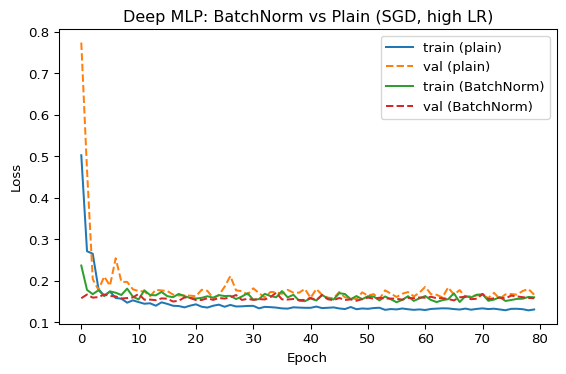

• Plain deep net:
  • Somewhat slower convergence and oscillating validation loss.
• With BatchNorm:
  • Smoother, more stable curves
  • Can tolerate higher learning rate before exploding

Summary

Evaluation & Quality Checks

When adding dropout / BatchNorm, always look at:

• Training vs validation curves
  • Did validation loss/accuracy improve or get more stable?
• Sensitivity to hyperparameters
  • After adding BatchNorm, can you:
    • Increase learning rate?
    • Reduce sensitivity to initialization?
• Overfitting vs underfitting
  • Too much dropout → underfitting
  • No regularization → overfitting
• Decision context
  • Are improvements meaningful for the actual task?
  • Use appropriate metrics (accuracy, F1, calibration plots, etc.)

🔬 Why BatchNorm Helps Gradients

Rough intuition:

• Backprop through a deep stack of affine + nonlinearity:
  • Gradients can shrink / grow depending on weight scales and activations.
• BatchNorm normalizes activations per layer:
  • Keeps them in a relatively stable range (mean ≈ 0, variance ≈ 1).
  • This reduces the risk that gradients become extremely tiny or huge in early layers.

Informal effect:

• Acts like a reparameterization of the optimization problem.
• Gradients with respect to unnormalized parameters flow through normalized activations, often leading to:
  • Better-conditioned Jacobians
  • More isotropic gradient directions

Warning

This is not a guarantee of good gradients—but empirically it helps many architectures.

🔬 Training Tricks

Common, simple tricks you’ll see in practice:

• Early stopping
  • Stop training when validation loss stops improving.
• Learning-rate schedules
  • Step decay, cosine annealing, warmup, etc.
• Gradient clipping
  • E.g., clip global norm to prevent rare explosions.
• Weight decay
  • L2 penalty through optimizer (e.g. AdamW).
• Careful initialization
  • Xavier/He initialization to keep variance stable.

Warning

• These interact with dropout & BatchNorm:
  • E.g., very strong weight decay + large dropout probability may be redundant / too strong.

Quick Check

1. Conceptual (MCQ)
   Dropout primarily helps by:

   • A. Increasing model capacity
     
   • B. Acting like an ensemble of thinned networks and reducing co-adaptation
     
   • C. Making gradients exactly zero in early layers
     
   • D. Eliminating the need for good data
     

2. Short answer
   In one sentence, what are the two learned parameters in BatchNorm and what do they do?
   

3. Conceptual (MCQ)
   You add dropout with \(p=0.5\) to a small model on a tiny dataset. Training and validation accuracy both drop sharply and stay low. What is the most likely diagnosis?

   • A. Underfitting caused by too much regularization
     
   • B. Data leakage
     
   • C. Exploding gradients
     
   • D. Incorrect loss function
     

4. Short numeric reasoning
   Suppose a hidden unit has activation \(h = 2.0\). With inverted dropout keep probability \(p = 0.5\), what are the possible training-time activations for this unit and their probabilities?
   

References

Gal, Yarin, and Zoubin Ghahramani. 2016. “Dropout as a Bayesian Approximation: Representing Model Uncertainty in Deep Learning.” In Proceedings of the 33rd International Conference on Machine Learning, 1050–59. ICML.

Ioffe, Sergey, and Christian Szegedy. 2015. “Batch Normalization: Accelerating Deep Network Training by Reducing Internal Covariate Shift.” In Proceedings of the 32nd International Conference on Machine Learning (ICML), 448–56. JMLR.org.

Srivastava, Nitish, Geoffrey Hinton, Alex Krizhevsky, Ilya Sutskever, and Ruslan Salakhutdinov. 2014. “Dropout: A Simple Way to Prevent Neural Networks from Overfitting.” Journal of Machine Learning Research 15 (56): 1929–58.