M31: Backpropagation & Automatic Differentiation
CSCI 3151 — Foundations of Machine Learning
Frank Rudzicz
Learning outcomes
By the end of this module, you should be able to:
- Explain the idea of a computational graph, forward pass, and backward pass.
- Apply the chain rule to derive gradients in a small feedforward network.
- 🔬 Implement manual backpropagation for a toy MLP and verify it with numerical gradient checks.
- Use an automatic differentiation framework to train the same model and interpret its gradient machinery.
- Diagnose common gradient-related bugs (e.g., wrong shapes, forgetting to reset gradients) using loss curves and gradient checks.
Motivation: Backprop
- We know how to train simple models (e.g., logistic regression) with gradient descent.
- For neural networks the loss depends on parameters via many layers of composition: \[ L(\theta) = \mathcal{L}(f_\theta(x), y) \]
- A naïve approach: symbolically differentiate the whole expression by hand.
- Tedious.
- Error-prone.
- Must be redone for every architecture.
- Backpropagation (Rumelhart, Hinton, and Williams 1986):
- A general recipe to compute all needed gradients efficiently.
- Re-uses intermediate quantities from the forward pass.
- Underlies modern deep learning and autodiff libraries.
Conceptual scaffold
Key definitions
- Computational graph
- Directed acyclic graph (DAG) where:
- Nodes = variables / intermediate values.
- Edges = functions mapping parent values to child values.
- Directed acyclic graph (DAG) where:
- Forward pass
- Evaluate the graph from inputs → output (e.g., loss).
- Store intermediate results needed later.
- Backward pass
- Propagate derivatives backwards from the loss: \[ \frac{\partial L}{\partial\text{node}} \]
- Use the chain rule at each node.
- Local gradient
- Derivative of a node with respect to its immediate parents.
- Backprop multiplies local gradients along paths.
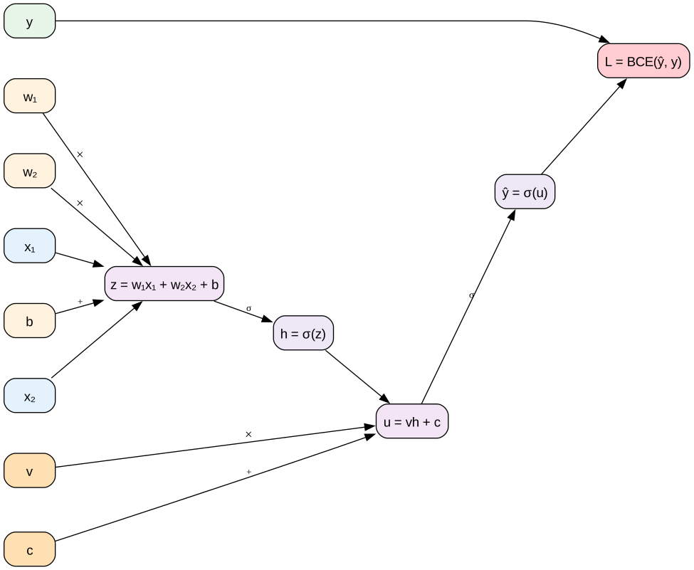
Visually
- Inputs
- \(x = (x_1, x_2)\): 2D input features.
- \(y \in \{0,1\}\): binary target label.
- Parameters
- \(w_1, w_2 \in \mathbb{R}\): weights from \(x_1, x_2\) into the hidden unit.
- \(b \in \mathbb{R}\): bias of the hidden unit.
- \(v \in \mathbb{R}\): weight from hidden unit \(h\) to the output pre-activation \(u\).
- \(c \in \mathbb{R}\): bias of the output unit.
- Intermediate quantities
- \(z = w_1 x_1 + w_2 x_2 + b\): hidden pre-activation.
- \(h = \sigma(z)\): hidden activation (elementwise sigmoid \(\sigma\)).
- \(u = v h + c\): output pre-activation.
- \(\hat{y} = \sigma(u)\): predicted probability for class \(1\).
- Loss
- \(L = \text{BCE}(\hat{y}, y)\): binary cross-entropy loss, \[ \text{BCE}(\hat{y}, y) = -\big[y \log \hat{y} + (1-y)\log(1-\hat{y})\big]. \]
Chain rule refresher
For scalar functions:
- If \(z = g(y)\) and \(y = f(x)\), then: \[ \frac{dz}{dx} = \frac{dz}{dy} \cdot \frac{dy}{dx} \]
For a computational graph:
- Each node has value \(v\) and parents \(\{u_i\}\).
- Local gradient: \(\partial v / \partial u_i\).
- Backprop computes: \[ \frac{\partial L}{\partial u_i} = \frac{\partial L}{\partial v} \cdot \frac{\partial v}{\partial u_i} \]
🤔
Think of \(\partial L / \partial v\) as a message flowing backward through the graph, scaled by local derivatives.
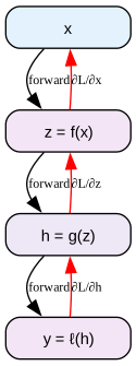
Backprop as message passing
For each node \(v\) in the computational graph:
- Forward pass
- Compute \[ v = f(u_1, \dots, u_k) \] where \(u_1, \dots, u_k\) are the parents of \(v\).
- Store both the value \(v\) and (often) pointers to its parents \(u_i\).
- Backward pass (message passing)
- By the time we visit \(v\) in backprop, we already know its gradient \[ \frac{\partial L}{\partial v}. \]
- For each parent \(u_i\), we compute the contribution from the path \(u_i \to v \to L\): \[ \delta_{u_i \leftarrow v} = \frac{\partial L}{\partial v} \cdot \frac{\partial v}{\partial u_i}. \]
- Then we accumulate this into the parent’s gradient: \[ \frac{\partial L}{\partial u_i} \leftarrow \frac{\partial L}{\partial u_i} + \delta_{u_i \leftarrow v}. \]
- Reverse topological order
- We process nodes from outputs back to inputs.
- Each parent collects contributions from all of its children.
🔑 Key idea
Backprop is local message passing: each node sends a gradient message upstream to its parents, and each parent sums all messages it receives.
🔬 node with multiple children
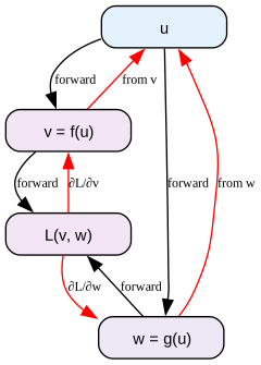
Suppose a node \(u\) feeds into two children \(v\) and \(w\):
- \(v = f(u)\)
- \(w = g(u)\)
- The loss depends on both: \(L = L(v, w)\).
Then by the chain rule, \[ \frac{\partial L}{\partial u} = \frac{\partial L}{\partial v} \frac{\partial v}{\partial u} + \frac{\partial L}{\partial w} \frac{\partial w}{\partial u}. \]
In message-passing / code form:
- Initialize gradients to zero: \[ \frac{\partial L}{\partial u} = 0. \]
- When backprop visits \(v\): \[ \frac{\partial L}{\partial u} \leftarrow \frac{\partial L}{\partial u} + \frac{\partial L}{\partial v} \frac{\partial v}{\partial u}. \]
- When backprop visits \(w\): \[ \frac{\partial L}{\partial u} \leftarrow \frac{\partial L}{\partial u} + \frac{\partial L}{\partial w} \frac{\partial w}{\partial u}. \]
After both messages have arrived, the stored \(\frac{\partial L}{\partial u}\) equals the full derivative above.
🧠 Mental model
Each child sends a gradient message to \(u\). Backprop simply adds up all such messages.
❌ “Backprop by hand” gone wrong
Common misuse / failure mode:
- You derive gradients once on paper for a specific network (say, 1 hidden layer).
- You hard-code the resulting formulas (e.g., explicit partials for every weight).
- Then you:
- Change the architecture (add a layer, new activation).
- Or reuse code on a different model.
- Result: gradients no longer match the computation graph.
- Training fails or behaves strangely.
- Debugging is painful.
Lesson
Treat backprop as a general algorithm on graphs, not a one-off symbolic calculation.
Modern frameworks rebuild the graph at runtime and re-run backprop automatically.
Math lens
Tiny MLP gradients
We’ll derive gradients for a single training example \((x, y)\).
- Input \(x \in \mathbb{R}^d\)
- Hidden layer: \[ a = W x + b \quad (W \in \mathbb{R}^{m\times d},\; b \in \mathbb{R}^m) \] \[ h = \sigma(a) \quad (\text{elementwise}) \]
- Output (binary classification): \[ u = v^\top h + c \quad (v \in \mathbb{R}^m,\; c \in \mathbb{R}) \] \[ \hat{y} = \sigma(u) \]
- Loss (binary cross-entropy): \[ L = -[y \log \hat{y} + (1-y)\log(1-\hat{y})] \]
Step 1: gradient at the output
For logistic + BCE, a key simplification:
\[ \hat{y} = \sigma(u) = \frac{1}{1+e^{-u}} \]
For a single training example with BCE loss and sigmoid output, we can show:
\[ \ell(\hat{y}, y) = -[y \log \hat{y} + (1-y)\log(1-\hat{y})] \quad\Rightarrow\quad \frac{\partial \ell}{\partial u} = \hat{y} - y. \]
Later, when we average over a mini-batch, this gradient picks up a factor (1/n). We’ll see that in the code.
Note
This “\(\hat{y} - y\)” term appears in many logistic / softmax models.
Step 2: propagate to \(v\) and \(h\)
We have:
- \(u = v^\top h + c\)
Local gradients:
\[ \frac{\partial u}{\partial v} = h,\quad \frac{\partial u}{\partial h} = v \]
Backprop:
\[ \frac{\partial L}{\partial v} = \frac{\partial L}{\partial u} \cdot \frac{\partial u}{\partial v} = (\hat{y} - y)\, h \]
\[ \frac{\partial L}{\partial h} = \frac{\partial L}{\partial u} \cdot \frac{\partial u}{\partial h} = (\hat{y} - y)\, v \]
\[ \frac{\partial L}{\partial c} = \frac{\partial L}{\partial u} \cdot \frac{\partial u}{\partial c} = \hat{y} - y \]
Step 3: propagate to \(W\), \(b\)
Recall:
- \(h = \sigma(a)\)
- \(a = W x + b\)
Elementwise:
\[ h_j = \sigma(a_j),\quad a_j = w_j^\top x + b_j \] (where \(w_j\) is row \(j\) of \(W\)).
Local gradients:
\[ \frac{\partial h_j}{\partial a_j} = \sigma'(a_j) = h_j (1 - h_j) \quad \text{for sigmoid} \]
Then:
\[ \frac{\partial L}{\partial a_j} = \frac{\partial L}{\partial h_j}\cdot \frac{\partial h_j}{\partial a_j} \]
\[ \frac{\partial L}{\partial w_j} = \frac{\partial L}{\partial a_j} \cdot \frac{\partial a_j}{\partial w_j} = \frac{\partial L}{\partial a_j}\, x^\top \]
\[ \frac{\partial L}{\partial b_j} = \frac{\partial L}{\partial a_j} \]
In matrix form:
\[ \frac{\partial L}{\partial W} = \left(\frac{\partial L}{\partial a}\right) x^\top \]
Note
Automatic differentiation (autodiff) is a way to automatically compute exact derivatives of a function implemented as code, by applying the chain rule along its computation graph.
Reverse-mode vs forward-mode autodiff
- Forward-mode autodiff
- Tracks how each intermediate changes with respect to a small set of inputs.
- Best when you have few inputs and many outputs
(e.g., differentiating a simulation w.r.t. a handful of parameters).
- Reverse-mode autodiff (backprop)
- Tracks how a scalar output (like a loss \(L\)) changes with respect to many inputs/parameters.
- Best when you have many parameters and one loss
→ exactly the deep-learning setting.
- Modern ML libraries (PyTorch, JAX, TensorFlow) all:
- Build a computation graph during the forward pass (Baydin et al. 2018; Griewank and Walther 2008).
- Store the operations and intermediate values.
- Run reverse-mode on that graph to compute \(\partial L / \partial \theta\) for every parameter \(\theta\).
Example 1: Manual backprop in Numpy
💪 Setup
We’ll use a subset of the classic two moons dataset for binary classification.
Code
import numpy as np
import pandas as pd
import matplotlib.pyplot as plt
from sklearn.datasets import make_moons
from sklearn.model_selection import train_test_split

# Reproducibility
rng = np.random.default_rng(3151)

X, y = make_moons(n_samples=400, noise=0.2, random_state=3151)
X_train, X_val, y_train, y_val = train_test_split(
    X, y, test_size=0.25, random_state=3151, stratify=y
)

X_train.shape, X_val.shape
((300, 2), (100, 2))💪 Visualizing the data
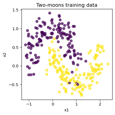
💪 Implementing the tiny MLP
We use 2 input features, a small hidden layer, and 1 output:
Code
def sigmoid(x):
    return 1 / (1 + np.exp(-x))

def sigmoid_deriv(x):
    s = sigmoid(x)       # technically, this is not great -- we'd compute sigmoid externally and reuse it here
    return s * (1 - s)

def bce_loss(y_hat, y_true, eps=1e-8):
    y_hat = np.clip(y_hat, eps, 1 - eps)
    return -np.mean(y_true * np.log(y_hat) + (1 - y_true) * np.log(1 - y_hat))

d = 2      # input dim
m = 8      # hidden units
rng = np.random.default_rng(0)

# Initialize parameters
W = rng.normal(scale=0.5, size=(m, d))
b = np.zeros(m)
v = rng.normal(scale=0.5, size=(m,))
c = 0.0

def forward(X):
    """
    X: (n, d)
    returns (a, h, u, y_hat)
    """
    a = X @ W.T + b          # (n, m)
    h = sigmoid(a)           # (n, m)
    u = h @ v + c            # (n,)
    y_hat = sigmoid(u)       # (n,)
    return a, h, u, y_hat
💪 One training step with manual backprop
Code
def train_step(X_batch, y_batch, W, b, v, c, lr=0.1):
    n = X_batch.shape[0]
    # Forward pass
    a, h, u, y_hat = forward(X_batch)
    loss = bce_loss(y_hat, y_batch)

    # Backward pass
    # dL/du
    dL_du = (y_hat - y_batch) / n  # (n,); here we're taking an average over the batch, as foretold

    # dL/dv and dL/dc
    dL_dv = h.T @ dL_du            # (m,)
    dL_dc = np.sum(dL_du)          # scalar

    # dL/dh
    dL_dh = np.outer(dL_du, v)     # (n, m)

    # dL/da via sigmoid derivative
    dL_da = dL_dh * sigmoid_deriv(a)  # (n, m)

    # dL/dW, dL/db
    dL_dW = dL_da.T @ X_batch      # (m, d)
    dL_db = np.sum(dL_da, axis=0)  # (m,)

    # Gradient step
    W -= lr * dL_dW
    b -= lr * dL_db
    v -= lr * dL_dv
    c -= lr * dL_dc

    return loss, W, b, v, c
💪 Training loop & loss curves
Code
def train_manual(X_train, y_train, X_val, y_val,
                 epochs=200, batch_size=64, lr=0.1):
    global W, b, v, c
    n = X_train.shape[0]
    history = {"epoch": [], "train_loss": [], "val_loss": []}
    rng = np.random.default_rng(1)

    for epoch in range(1, epochs + 1):
        # Mini-batch SGD
        perm = rng.permutation(n)
        X_shuff = X_train[perm]
        y_shuff = y_train[perm]

        for i in range(0, n, batch_size):
            X_batch = X_shuff[i:i+batch_size]
            y_batch = y_shuff[i:i+batch_size]
            loss, W, b, v, c = train_step(
                X_batch, y_batch, W, b, v, c, lr=lr
            )

        # Track losses
        _, _, _, y_hat_train = forward(X_train)
        _, _, _, y_hat_val = forward(X_val)
        train_loss = bce_loss(y_hat_train, y_train)
        val_loss = bce_loss(y_hat_val, y_val)

        history["epoch"].append(epoch)
        history["train_loss"].append(train_loss)
        history["val_loss"].append(val_loss)

    return pd.DataFrame(history)

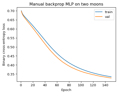
hist_df = train_manual(X_train, y_train, X_val, y_val,
                       epochs=150, batch_size=64, lr=0.1)
hist_df.tail()| epoch | train_loss | val_loss | |
|---|---|---|---|
| 145 | 146 | 0.336593 | 0.329225 |
| 146 | 147 | 0.336040 | 0.328634 |
| 147 | 148 | 0.335487 | 0.328349 |
| 148 | 149 | 0.334935 | 0.328013 |
| 149 | 150 | 0.334407 | 0.327439 |
💪 Loss curve plot
💪 Table: losses over time
Code
| epoch | train_loss | val_loss | |
|---|---|---|---|
| 0 | 1 | 0.700650 | 0.698315 |
| 1 | 31 | 0.574500 | 0.556877 |
| 2 | 61 | 0.461064 | 0.439762 |
| 3 | 91 | 0.391449 | 0.375889 |
| 4 | 121 | 0.354569 | 0.345354 |
✏️ Consider:
- Is training converging?
- Does validation loss mirror training loss?
- What might we change if loss is noisy or diverging?
💪 Gradient checking: quality assurance
Before trusting our manual backprop, we can compare to finite differences.
Idea
For a scalar parameter \(\theta\):
\[ \frac{\partial L}{\partial \theta} \approx \frac{L(\theta + \epsilon) - L(\theta - \epsilon)}{2\epsilon} \]
For a tiny network and tiny batch, we can numerically approximate gradients and compare them to our backprop outputs.
Example gradient check (one parameter)
Code
def loss_for_params(W, b, v, c, X_batch, y_batch):
    _, _, _, y_hat = forward(X_batch)
    return bce_loss(y_hat, y_batch)

# Pick a tiny batch
X_small = X_train[:5]
y_small = y_train[:5]

# Compute backprop gradient for v[0]
_, h, u, y_hat = forward(X_small)
dL_du = (y_hat - y_small) / len(X_small)
dL_dv_backprop = (h.T @ dL_du)[0]  # gradient for v[0]

# Finite difference gradient
eps = 1e-5
v_perturb = v.copy()
v_perturb[0] += eps
loss_plus = loss_for_params(W, b, v_perturb, c, X_small, y_small)

v_perturb[0] -= 2 * eps
loss_minus = loss_for_params(W, b, v_perturb, c, X_small, y_small)

dL_dv_fd = (loss_plus - loss_minus) / (2 * eps)
dL_dv_backprop, dL_dv_fd
(np.float64(0.043839416812162045), np.float64(0.0))If these two numbers are close (e.g., relative error < 1e-3), our gradient for that parameter is likely correct.
💪 Small gradient check table
Code
def check_grad_v_component(idx, eps=1e-5):
    X_small = X_train[:5]
    y_small = y_train[:5]

    # Backprop
    _, h, u, y_hat = forward(X_small)
    dL_du = (y_hat - y_small) / len(X_small)
    dL_dv_backprop = (h.T @ dL_du)[idx]

    # Finite difference
    v_perturb = v.copy()
    v_perturb[idx] += eps
    loss_plus = loss_for_params(W, b, v_perturb, c, X_small, y_small)

    v_perturb[idx] -= 2 * eps
    loss_minus = loss_for_params(W, b, v_perturb, c, X_small, y_small)

    dL_dv_fd = (loss_plus - loss_minus) / (2 * eps)
    rel_err = np.abs(dL_dv_backprop - dL_dv_fd) / (np.abs(dL_dv_fd) + 1e-8)
    return dL_dv_backprop, dL_dv_fd, rel_err

rows = []
for idx in range(min(5, len(v))):
    g_back, g_fd, rel_err = check_grad_v_component(idx)
    rows.append({
        "index": idx,
        "grad_backprop": g_back,
        "grad_finite_diff": g_fd,
        "relative_error": rel_err
    })

pd.DataFrame(rows)| index | grad_backprop | grad_finite_diff | relative_error | |
|---|---|---|---|---|
| 0 | 0 | 0.043839 | 0.0 | 4.383942e+06 |
| 1 | 1 | 0.031211 | 0.0 | 3.121084e+06 |
| 2 | 2 | 0.039205 | 0.0 | 3.920467e+06 |
| 3 | 3 | 0.005649 | 0.0 | 5.648833e+05 |
| 4 | 4 | 0.014880 | 0.0 | 1.488018e+06 |
Interpretation:
- If relative errors are small → backprop seems trustworthy.
- Large discrepancies → bug in backprop or numerical issues.
Worked example 2: Autograd with PyTorch
Motivation
Instead of:
Manually implementing derivatives for each layer, autodiff lets us:
- Define the forward computation.
- Ask the framework to compute gradients of a scalar loss w.r.t. parameters.
We’ll repeat the two-moons experiment using PyTorch, and compare:
- Loss curves
- Simplicity of code
- Where we still need to be careful
PyTorch setup
Code
import torch
from torch import nn
from torch.utils.data import TensorDataset, DataLoader

torch.manual_seed(3151)

X_train_t = torch.tensor(X_train, dtype=torch.float32)
y_train_t = torch.tensor(y_train, dtype=torch.float32).unsqueeze(1)
X_val_t   = torch.tensor(X_val, dtype=torch.float32)
y_val_t   = torch.tensor(y_val, dtype=torch.float32).unsqueeze(1)

train_ds = TensorDataset(X_train_t, y_train_t)
val_ds   = TensorDataset(X_val_t, y_val_t)

train_loader = DataLoader(train_ds, batch_size=64, shuffle=True)
val_loader   = DataLoader(val_ds, batch_size=256, shuffle=False)
What is a tensor (in PyTorch)?
In PyTorch, a tensor is just a multi-dimensional array of numbers, very much like a NumPy ndarray, but with extra powers:
- It can live on CPU or GPU memory.
- PyTorch can track operations on tensors so it can automatically compute gradients.
- Shapes like:
- scalar:
()
- vector:
(d,)
- matrix:
(m, d)
- batch of inputs:
(n, d)
- scalar:
We’ll mostly use 2D and 3D tensors (batches of feature vectors, or batches of images).
For more details: see 🔗PyTorch Tensors docs.
Model & optimizer
Code
class TinyMLP(nn.Module):
    def __init__(self, d_in=2, d_hidden=8):
        super().__init__()
        self.net = nn.Sequential(
            nn.Linear(d_in, d_hidden),
            nn.Sigmoid(),
            nn.Linear(d_hidden, 1),
            nn.Sigmoid()
        )

    def forward(self, x):
        return self.net(x)

model = TinyMLP()
criterion = nn.BCELoss()
optimizer = torch.optim.SGD(model.parameters(), lr=0.1)
Training loop with autograd
Code
def train_with_autograd(model, train_loader, val_loader, epochs=50):
    history = {"epoch": [], "train_loss": [], "val_loss": []}

    for epoch in range(1, epochs + 1):
        model.train()
        running_loss = 0.0
        n_train = 0

        for Xb, yb in train_loader:
            optimizer.zero_grad()        # IMPORTANT: clear old gradients
            yhat = model(Xb)
            loss = criterion(yhat, yb)
            loss.backward()              # backprop: compute gradients
            optimizer.step()             # SGD step

            running_loss += loss.item() * Xb.size(0)
            n_train += Xb.size(0)

        train_loss = running_loss / n_train

        # Validation
        model.eval()
        with torch.no_grad():
            val_loss = 0.0
            n_val = 0
            for Xb, yb in val_loader:
                yhat = model(Xb)
                loss = criterion(yhat, yb)
                val_loss += loss.item() * Xb.size(0)
                n_val += Xb.size(0)
        val_loss /= n_val

        history["epoch"].append(epoch)
        history["train_loss"].append(train_loss)
        history["val_loss"].append(val_loss)

    return pd.DataFrame(history)

hist_torch = train_with_autograd(model, train_loader, val_loader, epochs=80)
hist_torch.tail()| epoch | train_loss | val_loss | |
|---|---|---|---|
| 75 | 76 | 0.382846 | 0.366493 |
| 76 | 77 | 0.380768 | 0.364582 |
| 77 | 78 | 0.378781 | 0.362786 |
| 78 | 79 | 0.377215 | 0.361295 |
| 79 | 80 | 0.375253 | 0.359635 |
Comparing loss curves: manual vs autograd
Code
plt.figure(figsize=(5, 4))
plt.plot(hist_df["epoch"], hist_df["train_loss"], label="manual train", linestyle="--")
plt.plot(hist_df["epoch"], hist_df["val_loss"], label="manual val", linestyle="--")
plt.plot(hist_torch["epoch"], hist_torch["train_loss"], label="torch train")
plt.plot(hist_torch["epoch"], hist_torch["val_loss"], label="torch val")
plt.xlabel("Epoch")
plt.ylabel("BCE loss")
plt.title("Manual vs autograd training curves")
plt.legend()
plt.tight_layout()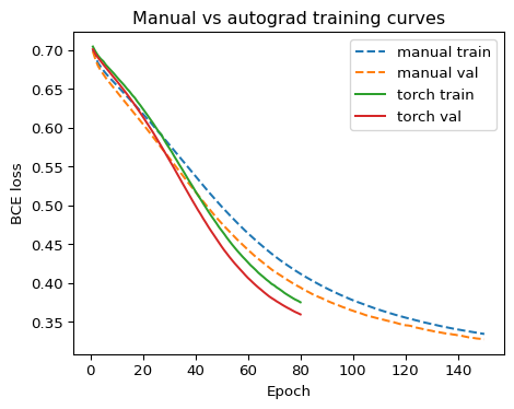
✏️
- Do curves look qualitatively similar?
- If not, what differences in initialization, learning rate, or batching might explain it?
- Where do you think is PyTorch doing “the same math” we did by hand?
Table: final performance comparison
Code
# Simple accuracy function
def accuracy_from_logits(model, X, y):
    model.eval()
    with torch.no_grad():
        logits = model(torch.tensor(X, dtype=torch.float32))
        preds = (logits.numpy().ravel() > 0.5).astype(int)
    return np.mean(preds == y)

acc_train_torch = accuracy_from_logits(model, X_train, y_train)
acc_val_torch   = accuracy_from_logits(model, X_val, y_val)

# For manual model, recompute predictions using the current W, b, v, c
_, _, _, yhat_train_manual = forward(X_train)
_, _, _, yhat_val_manual   = forward(X_val)

acc_train_manual = np.mean((yhat_train_manual > 0.5).astype(int) == y_train)
acc_val_manual   = np.mean((yhat_val_manual > 0.5).astype(int) == y_val)

pd.DataFrame({
    "model": ["manual MLP", "torch MLP"],
    "train_acc": [acc_train_manual, acc_train_torch],
    "val_acc": [acc_val_manual, acc_val_torch]
})| model | train_acc | val_acc | |
|---|---|---|---|
| 0 | manual MLP | 0.840000 | 0.82 |
| 1 | torch MLP | 0.823333 | 0.82 |
Wrap-up
Summary
Key takeaways:
- Backprop = chain rule on a computational graph, organized efficiently.
- It’s not just for neural networks!
- Manual derivations on toy models can build intuition and help debug.
- Autodiff frameworks automate gradient computation but do not remove the need for:
- Careful modelling.
- Sanity checks.
- Proper evaluation & diagnostics.
- Understanding backprop is essential for:
- Designing architectures,
- Debugging training,
- Engaging with modern deep learning research.
Evaluation & quality checks for backprop
When implementing or using backprop, we care about:
- Correctness of gradients
- Use unit tests & gradient checks (finite differences).
- Compare manual and autodiff implementations on tiny networks.
- Training behaviour
- Loss curves should decrease (at least initially).
- If loss diverges or oscillates wildly:
- Learning rate too high? Gradients exploding? Bug in forward/backward pass?
- Sanity checks
- Zero-initialize weights? (usually bad; symmetry)
- Random labels? Model should not learn much.
- Shuffle labels and see if model behaves differently.
Common gradient-related bugs 🐜
- Forgetting to reset gradients (e.g., missing
optimizer.zero_grad()):- Gradients accumulate across batches.
- Loss might decrease strangely or explode.
- Incorrect broadcasting / shapes
- Summing over wrong axis, mixing batch and feature dims.
- Works in code but gives wrong updates.
- Non-differentiable operations in the path
- Hard
argmax, control-flow that breaks the graph. - Framework can’t propagate gradients as expected.
- Hard
- Detach / no-grad misused
- Accidentally cutting the graph (
.detach()/no_gradin the wrong place). - Gradients become zero for some parameters.
- Accidentally cutting the graph (
Ethics & risks
Backprop and autodiff are technical tools, but how they’re used matters:
- Opaque decision-making
- Complex networks with millions of parameters are hard to interpret.
- Backprop encourages very flexible models; extra care needed for explainability.
- Silent bugs & hidden bias
- Incorrect gradient implementations may silently mis-train a model.
- Even with correct gradients, training amplifies patterns in data:
- Biased data ⇒ biased gradients ⇒ biased models.
- Reproducibility & accountability
- Small changes in initialization or training setup can change outcomes.
- For high-stakes applications, document:
- Code versions, random seeds, hyperparameters, training curves.
🔎 Mitigations
- Run gradient checks and sanity experiments.
- Inspect metrics across subgroups where possible.
- Log experiments (e.g., with MLFlow) for traceability.
How libraries actually implement autodiff
Frameworks like PyTorch tend to:
- Record operations during forward pass
- Each tensor knows which operation produced it and which tensors were inputs.
- Build a dynamic computation graph
- Nodes: tensors; edges: operations.
- Backward call
- Start from a scalar loss.
- Traverse the graph in reverse topological order.
- Call each operation’s pre-defined backward rule (local gradient).
- Accumulate gradients on parameters
- Each leaf tensor with
requires_grad=Truegets a.gradattribute filled in.
- Each leaf tensor with
You get all this “for free” – but only if the forward pass is correct.
Quick-check
Q1 (MCQ)
For training neural networks, which mode of automatic differentiation is typically most efficient?
A. Symbolic differentiation
B. Forward-mode autodiff
C. Reverse-mode autodiff (backprop)
D. Finite-difference approximation
Q2 (conceptual)
In a 1-hidden-layer MLP trained with BCE loss and sigmoid output, why does the term \((\hat{y} - y)\) appear in the gradient with respect to the output pre-activation \(u\)?
- Brief explanation:
Q3 (short numeric)
Suppose for a single sample:
- \(\hat{y} = 0.8\), \(y = 1.0\),
- Hidden activation for unit \(j\): \(h_j = 0.5\),
- Output weight \(v_j = 2.0\),
- There are \(n = 10\) samples in the batch.
What is the contribution of this sample to \(\frac{\partial L}{\partial v_j}\)?
Assume: \[ \frac{\partial L}{\partial u} = \frac{\hat{y} - y}{n} \quad \text{and} \quad \frac{\partial L}{\partial v_j} = \frac{\partial L}{\partial u} \cdot h_j \]
Q4 (debugging)
You train a small MLP in PyTorch and observe:
- Loss decreases for a few batches.
- Then loss suddenly jumps up and becomes
nan.
Name two plausible explanations related to gradients or optimization.
References
Baydin, Atılım Güneş, Barak A. Pearlmutter, Alexey Andreyevich Radul, and Jeffrey Mark Siskind. 2018. “Automatic Differentiation in Machine Learning: A Survey.” Journal of Machine Learning Research 18.
Griewank, Andreas, and Andrea Walther. 2008. Evaluating Derivatives: Principles and Techniques of Algorithmic Differentiation. 2nd ed. SIAM. https://doi.org/10.1137/1.9780898717761.
Rumelhart, David E., Geoffrey E. Hinton, and Ronald J. Williams. 1986. “Learning Representations by Back-Propagating Errors.” Nature 323: 533–36.
