CSCI 3151 โ Foundations of Machine Learning
By the end of this module, you should be able to:
For input \(x \in \mathbb{R}^{d}\):
\[ f_{\text{linear}}(x) = w^\top x + b \]
\[ p(y=1 \mid x) = \sigma(w^\top x + b),\quad \sigma(z) = \frac{1}{1 + e^{-z}}. \]
Build a function by stacking simple transforms layer by layer.
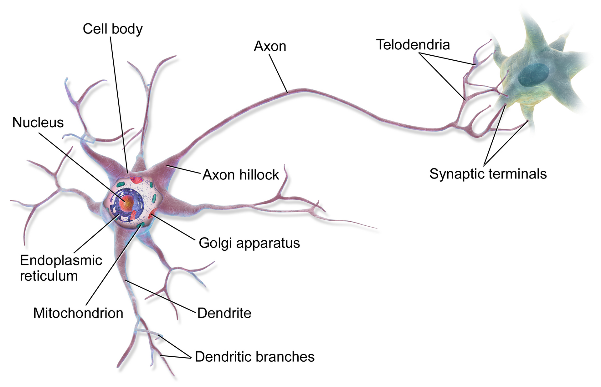
A biological neuron (very roughly):

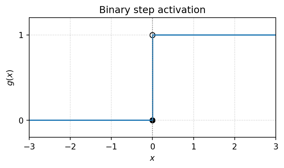
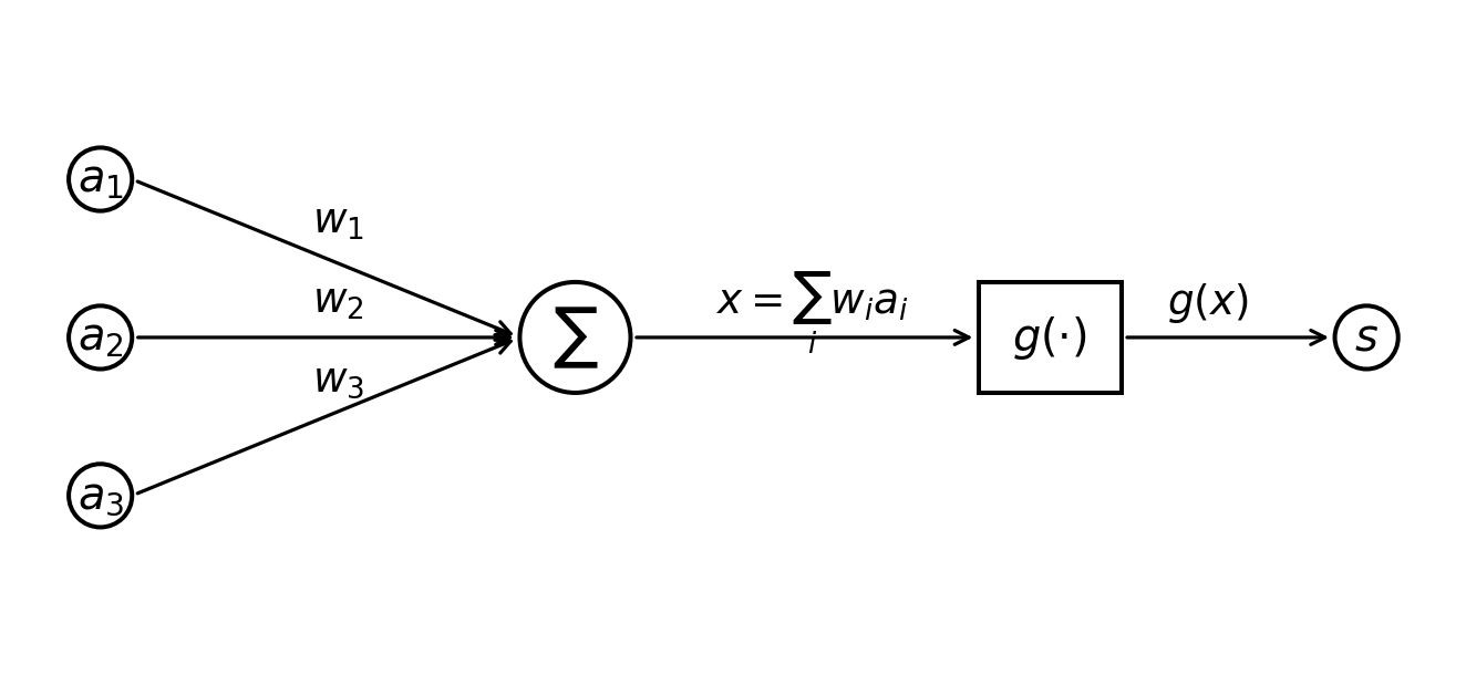
Artificial neuron (McCulloch and Pitts 1943):


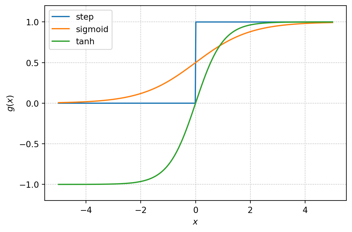
For differentiable training (gradient-based learning), smooth alternatives became popular:
๐ค Key ideas:
Later, rectified linear units (ReLUs) (Glorot, Bordes, and Bengio 2011) became the default for many deep nets:
ReLU: \[ g(x) = \max (0, x) \]
Its smooth cousin, softplus: \[ g(x) = \log\left(1+e^x\right) \]
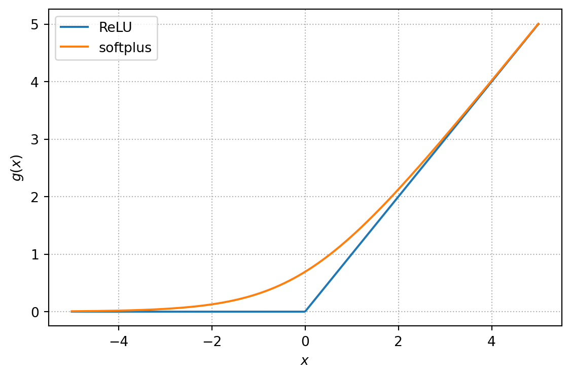
๐ค Why ReLUs?
Learning in a single perceptron (Rosenblatt 1958):
Note
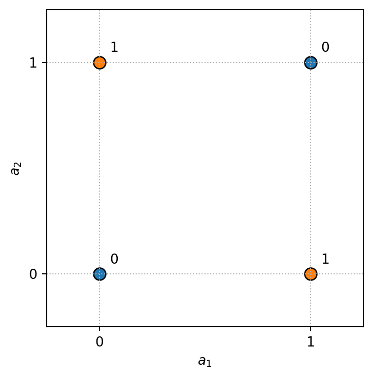
But there is a fundamental limitation (Minsky and Papert 1969):
Classic counterexample: XOR

This sets up the next step:
๐ง Mental picture
Feedforward = information flows one way; no loops, no recurrence
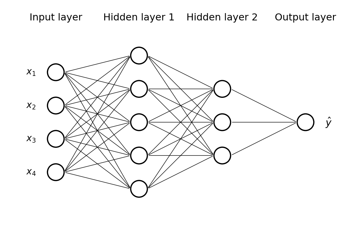
For an input \(x \in \mathbb{R}^{d_0}\),
Define:
\[ \begin{aligned} h_0 &= x \\ z_\ell &= W_\ell h_{\ell-1} + b_\ell \quad (\text{pre-activation}) \\ h_\ell &= g_\ell(z_\ell) \quad (\text{post-activation}) \end{aligned} \]
Proposition (non-trivial but short)
Consider a network with layers:
\[ h_1 = W_1 x + b_1,\quad h_2 = W_2 h_1 + b_2,\quad \ldots,\quad h_L = W_L h_{L-1} + b_L \]
and no nonlinearities (i.e., ๐ all \(g_\ell\) are identity๐). Then:
\[ h_L = W_{\text{eff}} x + b_{\text{eff}} \]
for some effective weight matrix \(W_{\text{eff}}\) and bias \(b_{\text{eff}}\); i.e., the whole network is just a single linear model.
Sketch of reasoning
\[ h_2 = W_2(W_1 x + b_1) + b_2 = (W_2 W_1)x + (W_2 b_1 + b_2) \]
Focus on a simple fully-connected network:
Total number of parameters:
\[ \sum_{\ell=1}^{L} \left( d_\ell \cdot d_{\ell-1} + d_\ell \right) \]
(since each layer has a weight matrix \(W_\ell\) and a bias \(b_\ell\))
Assume:
Logistic regression:
1-hidden-layer network:
Order-of-magnitude = more capacity to capture structure
Practical takeaway (for this course):
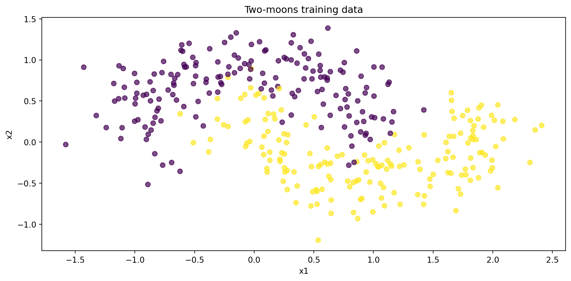
Weโll revisit the classic two-moons dataset:
import numpy as np
import matplotlib.pyplot as plt
from sklearn.datasets import make_moons
from sklearn.model_selection import train_test_split
X, y = make_moons(n_samples=500, noise=0.25, random_state=3151)
X_train, X_test, y_train, y_test = train_test_split(
X, y, test_size=0.3, random_state=3151, stratify=y
)
fig, ax = plt.subplots()
scatter = ax.scatter(X_train[:, 0], X_train[:, 1], c=y_train, alpha=0.7)
ax.set_xlabel("x1")
ax.set_ylabel("x2")
ax.set_title("Two-moons training data")
plt.tight_layout()
from sklearn.linear_model import LogisticRegression
from sklearn.metrics import accuracy_score
logreg = LogisticRegression()
logreg.fit(X_train, y_train)
y_train_pred = logreg.predict(X_train)
y_test_pred = logreg.predict(X_test)
print("Logistic regression accuracy:")
print(f" train: {accuracy_score(y_train, y_train_pred):.3f}")
print(f" test: {accuracy_score(y_test, y_test_pred):.3f}")
# Plot decision boundary
xx, yy = np.meshgrid(
np.linspace(X[:, 0].min() - 0.5, X[:, 0].max() + 0.5, 200),
np.linspace(X[:, 1].min() - 0.5, X[:, 1].max() + 0.5, 200),
)
grid = np.c_[xx.ravel(), yy.ravel()]
probs = logreg.predict_proba(grid)[:, 1].reshape(xx.shape)
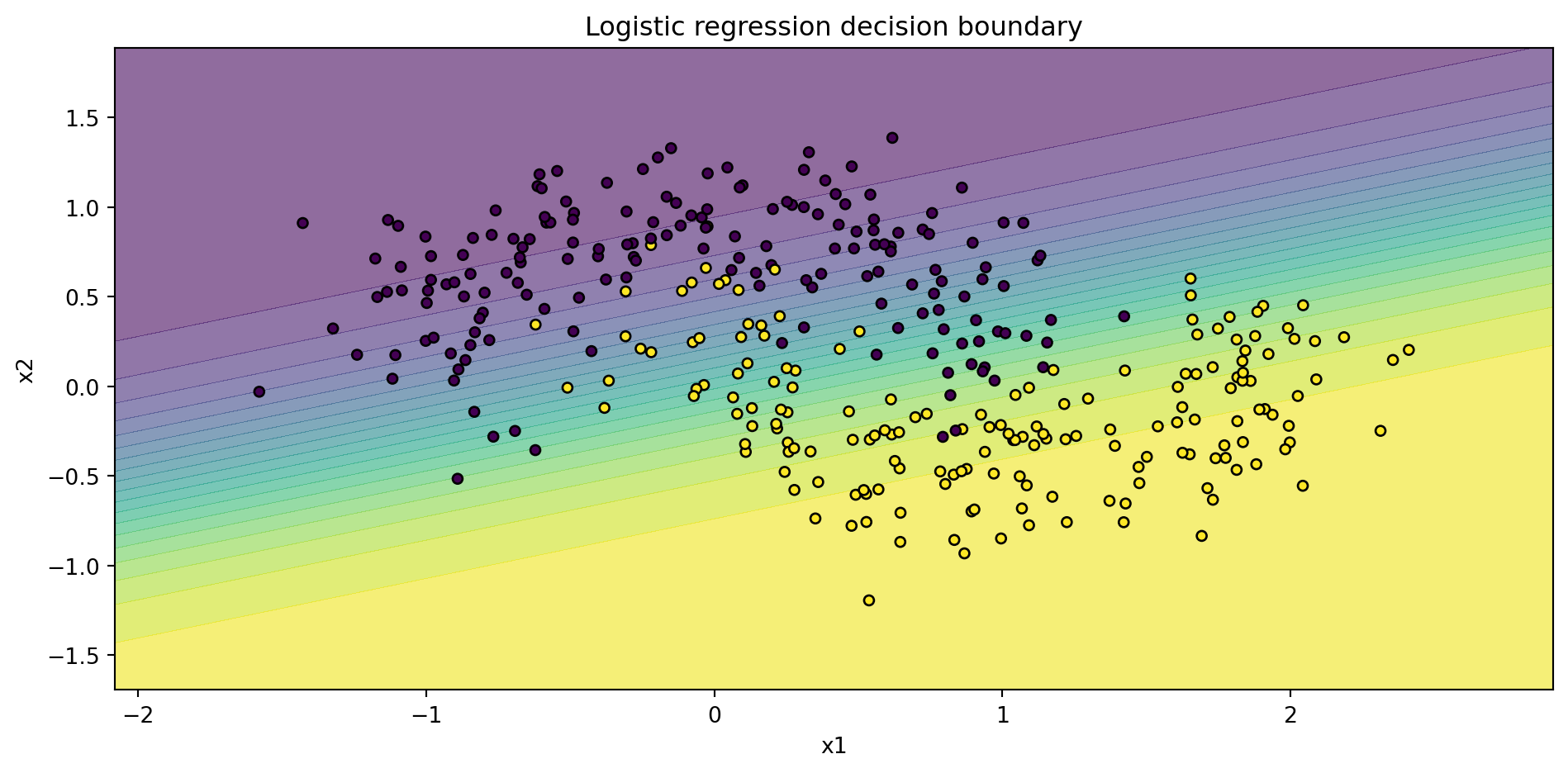
fig, ax = plt.subplots()
cs = ax.contourf(xx, yy, probs, levels=20, alpha=0.6)
scatter = ax.scatter(X_train[:, 0], X_train[:, 1], c=y_train, edgecolor="k", s=20)
ax.set_title("Logistic regression decision boundary")
ax.set_xlabel("x1")
ax.set_ylabel("x2")
plt.tight_layout()Logistic regression accuracy:
train: 0.860
test: 0.847
from sklearn.neural_network import MLPClassifier
mlp = MLPClassifier(
hidden_layer_sizes=(20,),
activation="relu",
solver="adam",
max_iter=500,
random_state=3151
)
mlp.fit(X_train, y_train)
y_train_pred_mlp = mlp.predict(X_train)
y_test_pred_mlp = mlp.predict(X_test)
print("MLP (20 hidden units, ReLU) accuracy:")
print(f" train: {accuracy_score(y_train, y_train_pred_mlp):.3f}")
print(f" test: {accuracy_score(y_test, y_test_pred_mlp):.3f}")
# Decision boundary
probs_mlp = mlp.predict_proba(grid)[:, 1].reshape(xx.shape)
fig, ax = plt.subplots()
cs = ax.contourf(xx, yy, probs_mlp, levels=20, alpha=0.6)
scatter = ax.scatter(X_train[:, 0], X_train[:, 1], c=y_train, edgecolor="k", s=20)
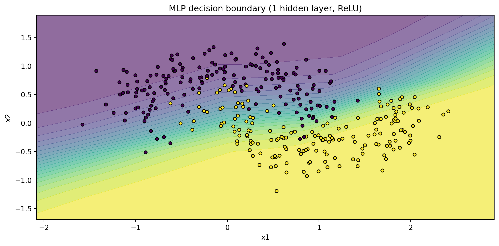
ax.set_title("MLP decision boundary (1 hidden layer, ReLU)")
ax.set_xlabel("x1")
ax.set_ylabel("x2")
plt.tight_layout()MLP (20 hidden units, ReLU) accuracy:
train: 0.874
test: 0.873

from sklearn.neural_network import MLPClassifier
mlp = MLPClassifier(
hidden_layer_sizes=(20,20,), # <- the only change is here!
activation="relu",
solver="adam",
max_iter=500,
random_state=3151
)
mlp.fit(X_train, y_train)
y_train_pred_mlp = mlp.predict(X_train)
y_test_pred_mlp = mlp.predict(X_test)
print("MLP (20 + 20 hidden units, ReLU) accuracy:")
print(f" train: {accuracy_score(y_train, y_train_pred_mlp):.3f}")
print(f" test: {accuracy_score(y_test, y_test_pred_mlp):.3f}")
# Decision boundary
probs_mlp = mlp.predict_proba(grid)[:, 1].reshape(xx.shape)
fig, ax = plt.subplots()
cs = ax.contourf(xx, yy, probs_mlp, levels=20, alpha=0.6)
scatter = ax.scatter(X_train[:, 0], X_train[:, 1], c=y_train, edgecolor="k", s=20)
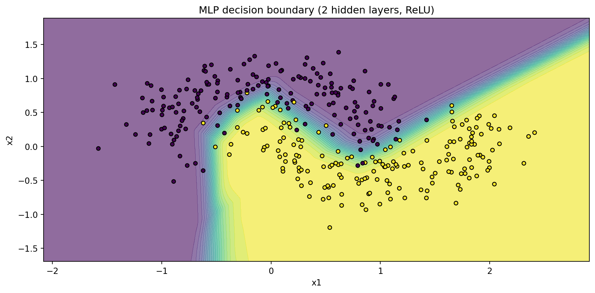
ax.set_title("MLP decision boundary (2 hidden layers, ReLU)")
ax.set_xlabel("x1")
ax.set_ylabel("x2")
plt.tight_layout()MLP (20 + 20 hidden units, ReLU) accuracy:
train: 0.966
test: 0.920

โ๏ธ Questions to ask:
Now back to the slightly more realistic handwritten digits dataset.
Goal:
from sklearn.datasets import load_digits
digits = load_digits()
X = digits.data # shape (n_samples, 64)
y = digits.target # labels 0โ9
print("Digits shape:", X.shape)
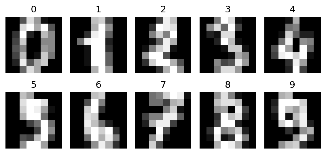
# Quick visual of a few digits
fig, axes = plt.subplots(2, 5, figsize=(6, 3))
for i, ax in enumerate(axes.ravel()):
ax.imshow(digits.images[i], cmap="gray")
ax.set_title(int(y[i]))
ax.axis("off")
plt.tight_layout()Digits shape: (1797, 64)

from sklearn.model_selection import train_test_split
from sklearn.preprocessing import StandardScaler
from sklearn.pipeline import Pipeline
X_train, X_temp, y_train, y_temp = train_test_split(
X, y, test_size=0.4, random_state=3151, stratify=y
)
X_val, X_test, y_val, y_test = train_test_split(
X_temp, y_temp, test_size=0.5, random_state=3151, stratify=y_temp
)
print("Train size:", X_train.shape[0])
print("Val size: ", X_val.shape[0])
print("Test size: ", X_test.shape[0])Train size: 1078
Val size: 359
Test size: 360
from sklearn.linear_model import LogisticRegression
from sklearn.metrics import accuracy_score
logreg_pipe = Pipeline([
("scaler", StandardScaler()),
("clf", LogisticRegression(
max_iter=1000,
multi_class="multinomial"
))
])
logreg_pipe.fit(X_train, y_train)
y_train_pred = logreg_pipe.predict(X_train)
y_val_pred = logreg_pipe.predict(X_val)
y_test_pred = logreg_pipe.predict(X_test)
logreg_results = {
"model": "Logistic regression",
"train_acc": accuracy_score(y_train, y_train_pred),
"val_acc": accuracy_score(y_val, y_val_pred),
"test_acc": accuracy_score(y_test, y_test_pred),
}
logreg_results{'model': 'Logistic regression',
'train_acc': 0.9981447124304267,
'val_acc': 0.9721448467966574,
'test_acc': 0.9666666666666667}
mlp_pipe = Pipeline([
("scaler", StandardScaler()),
("clf", MLPClassifier(
hidden_layer_sizes=(64,),
activation="relu",
alpha=1e-4, # L2 regularization
max_iter=500,
random_state=3151
))
])
mlp_pipe.fit(X_train, y_train)
y_train_pred_mlp = mlp_pipe.predict(X_train)
y_val_pred_mlp = mlp_pipe.predict(X_val)
y_test_pred_mlp = mlp_pipe.predict(X_test)
mlp_results = {
"model": "MLP (1 hidden layer, 64 units)",
"train_acc": accuracy_score(y_train, y_train_pred_mlp),
"val_acc": accuracy_score(y_val, y_val_pred_mlp),
"test_acc": accuracy_score(y_test, y_test_pred_mlp),
}
mlp_results{'model': 'MLP (1 hidden layer, 64 units)',
'train_acc': 1.0,
'val_acc': 0.9665738161559888,
'test_acc': 0.9666666666666667}
mlp_pipe = Pipeline([
("scaler", StandardScaler()),
("clf", MLPClassifier(
hidden_layer_sizes=(64,64,), # <- the only change
activation="relu",
alpha=1e-4, # L2 regularization
max_iter=500,
random_state=3151
))
])
mlp_pipe.fit(X_train, y_train)
y_train_pred_mlp = mlp_pipe.predict(X_train)
y_val_pred_mlp = mlp_pipe.predict(X_val)
y_test_pred_mlp = mlp_pipe.predict(X_test)
mlp2_results = {
"model": "MLP (2 hidden layers, 64+64 units)",
"train_acc": accuracy_score(y_train, y_train_pred_mlp),
"val_acc": accuracy_score(y_val, y_val_pred_mlp),
"test_acc": accuracy_score(y_test, y_test_pred_mlp),
}
mlp2_results{'model': 'MLP (2 hidden layers, 64+64 units)',
'train_acc': 1.0,
'val_acc': 0.9693593314763231,
'test_acc': 0.975}
| model | train_acc | val_acc | test_acc | |
|---|---|---|---|---|
| 0 | Logistic regression | 0.998145 | 0.972145 | 0.966667 |
| 1 | MLP (1 hidden layer, 64 units) | 1.000000 | 0.966574 | 0.966667 |
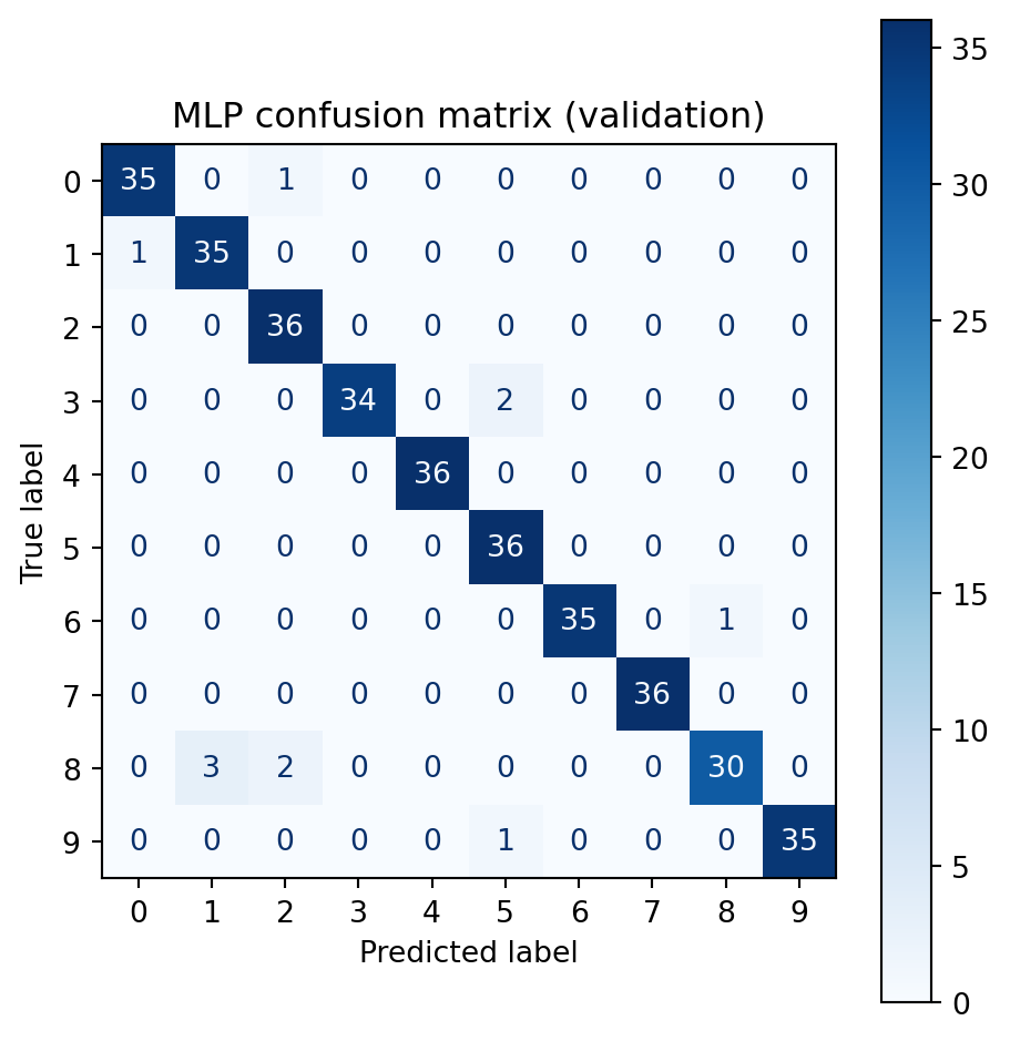
| 2 | MLP (2 hidden layers, 64+64 units) | 1.000000 | 0.969359 | 0.975000 |
Important
How many parameters did we just buy?
For digits: input dimension \(d=64\), classes \(K=10\).
For a fully-connected layer with \(n_{\ell-1}\to n_\ell\), params = \((n_{\ell-1}+1)n_\ell\) (weights + biases).
Logistic regression (softmax):
\(W\in\mathbb{R}^{K\times d},\ b\in\mathbb{R}^K \Rightarrow (d+1)K = (64+1)\cdot 10 = 650\)
MLP, 1 hidden layer (64):
\((64+1)\cdot 64 + (64+1)\cdot 10 = 4160 + 650 = 4810\)
MLP, 2 hidden layers (64+64):
\((64+1)\cdot 64 + (64+1)\cdot 64 + (64+1)\cdot 10 = 4160 + 4160 + 650 = 8970\)
Question: Look at your validation/test accuracies.
When using FFNNs, always keep the decision context in mind:
For our examples:
Note
PyTorch (build-your-own MLP)
torch.nn.Moduletorch.nn.Sequentialtorch.nn.Lineartorch.nn.DropoutLosses
torch.nn.CrossEntropyLosstorch.nn.MSELossโSolver choicesโ = optimizer choice
torch.optim.SGDtorch.optim.Adamtorch.optim.AdamWtorch.optim overviewoptimization tutorialRegularization & stability knobs (common)
weight_decay (L2 / weight decay) in optimizersDropout(p=...)scikit-learn
sklearn.neural_network.MLPClassifiersklearn.neural_network.MLPRegressorKey hyperparameters (the ones you actually tune)
hidden_layer_sizes=(...), activation={'relu','tanh','logistic','identity'}solver={'adam','sgd','lbfgs'}alpha (L2)learning_rate_init, batch_size, max_iter, tolearly_stopping=True, validation_fraction, n_iter_no_changePractical examples
Rule-of-thumb starting point
solver='adam', activation='relu', then tune alpha and learning_rate_init.Even simple FFNNs can be used in high-stakes settings (finance, health, hiring, etc.).
Q1 (MCQ)
Which of the following is not a reason we need nonlinear activations in neural networks?
A. To allow the network to represent more complex functions
B. To ensure that stacking layers does more than a single linear model
C. To make sure the loss function is convex
D. To avoid the composition of linear maps collapsing into one linear map
Q2
Consider a feedforward network with input dimension 5, one hidden layer of size 10, and a single output.
How many parameters (weights + biases) does it have?
Assume fully-connected layers and no tricks.
Q3 (MCQ)
On the moons dataset, suppose your MLP achieves:
Which diagnosis is most plausible?
A. Underfitting
B. Overfitting
C. Data leakage
D. Perfect model; no issues
Q4
On the digits dataset, your MLP and logistic regression have similar test accuracy, but the MLP takes much longer to train.
Give one reasonable explanation for why you might still prefer logistic regression in this setting.