M26: Linear dimensionality reduction & PCA

CSCI 3151 — Foundations of Machine Learning

Frank Rudzicz

Table of contents

• Conceptual scaffold
• Math lens
• Examples
• Final thoughts

Outcomes for M26

By the end of this module, you should be able to:

1. Explain what linear dimensionality reduction is and when PCA is an appropriate tool.
2. Define principal components in terms of variance maximization and reconstruction error.
3. Derive or follow the optimization problem whose solution gives PCA directions as eigenvectors of the covariance matrix.
4. Implement PCA in Python (with and without scikit-learn) and interpret explained variance ratios.
5. Evaluate the impact of PCA on downstream tasks (e.g., classification) and diagnose when PCA is helping vs hurting.

Motivation: why dimensionality reduction?

Common pain points with high-dimensional data:

• Computation:
  • Models get slower; optimization becomes harder.
• Overfitting:
  • Many features, relatively few samples → easier to memorize noise.
• Visualization:
  • Humans struggle beyond 2–3 dimensions.
• Redundancy:
  • Features can be highly correlated or nearly duplicated.

Dimensionality reduction tries to:

• Map \(x \in \mathbb{R}^d \to z \in \mathbb{R}^k\) with \(k \ll d\),
• Such that important structure in the data is retained.

PCA is the canonical linear method for this.

Conceptual scaffold

What is linear dimensionality reduction?

We assume:

• Data matrix \(X \in \mathbb{R}^{n \times d}\), with:
  • \(n\) examples (rows),
  • \(d\) features (columns),
  • Data is centered (zero mean per feature, e.g., by \(z\)-scoring).

Linear dimensionality reduction:

• Choose a matrix \(W \in \mathbb{R}^{d \times k}\) with \(k < d\).
• Project: \[ Z = X W \quad (\text{low-dimensional representation}) \]
• Optionally reconstruct: \[ \hat{X} = Z W^\top \]

🤔 Questions

• How do we choose good directions \(W\)?
• What does “good” even mean?

Projection & reconstruction

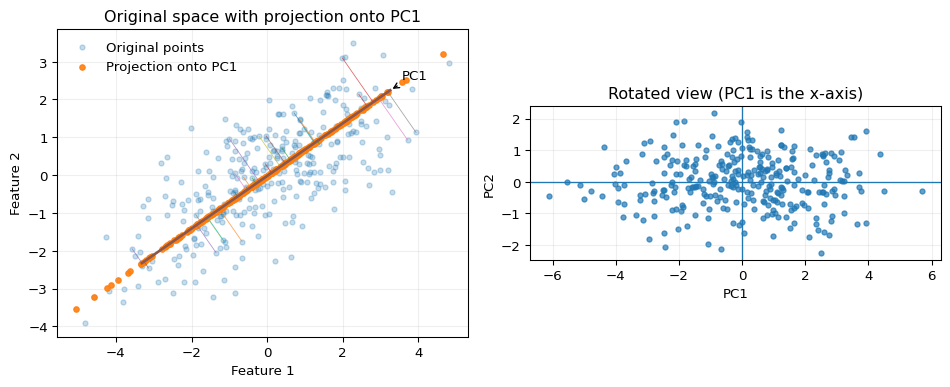
Left: original 2D cloud with projection onto the first principal component (PC1)
Right: the same cloud after rotating the plane so that PC1 is exactly the new x-axis.

Figure 1: Orthogonal projection onto the first principal component (left) and rotated view where PC1 is the x-axis (right).

PCA in one sentence

Principal Component Analysis (PCA) finds orthogonal directions in feature space:

• That capture as much variance as possible, and
  
• Equivalently, give the best linear low-rank approximation to the data.

The first principal component:

• The direction where the projected data has maximum variance.

Subsequent components:

• Maximize variance subject to being orthogonal to the earlier ones.

(a)

(b)

Figure 2

❌️ Anti-example: PCA misused as a preprocessing step

We have a tabular dataset with:

• age (years),
• income (dollars),
• num_visits (counts),
• has_disease (binary label).

A common but problematic workflow:

1. Concatenate all data (train + validation + test).
2. Fit PCA on this full matrix.
3. Transform everything with this PCA.
4. Use transformed features to train and evaluate a classifier.

✏️ What goes wrong?

• PCA “sees” the test set during fitting:
  • It learns directions optimized over all data, including future examples.
• Evaluation is optimistically biased:
  • You underestimate how much error you’ll see on truly new data.

This is a form of data leakage:
the representation itself is tuned using information from the test set.

✏️ Fix:

• Fit PCA only on the training data,
  then apply the learned transformation to validation/test.
• In scikit-learn: wrap PCA inside a Pipeline so that fit/transform happen with correct splits.

Math lens

🔬 PCA: data & covariance

Assume:

• Data matrix \(X \in \mathbb{R}^{n \times d}\) with rows \(x_i^\top\).
• Sample mean: \[ \mu = \frac{1}{n} \sum_{i=1}^n x_i \in \mathbb{R}^d. \]
• Centered data matrix: \[ \tilde X = X - \mathbf{1}\mu^\top, \] where \(\mathbf{1} \in \mathbb{R}^n\) is a column of ones.

Define the (empirical) covariance matrix: \[ \begin{aligned} \Sigma &= \frac{1}{n}\, \tilde X^\top \tilde X \\ &= \frac{1}{n} \sum_{i=1}^n (x_i - \mu)(x_i - \mu)^\top \in \mathbb{R}^{d \times d}. \end{aligned} \]

Note

Many stats texts use \(1/(n-1)\) instead of \(1/n\).
For PCA this only rescales the eigenvalues, not the principal directions.

For any unit vector \(w \in \mathbb{R}^d\) with \(\|w\|_2 = 1\):

• The scalar coordinate of \(x_i\) along direction \(w\) is \[ z_i = w^\top (x_i - \mu). \]
• The orthogonal projection of \(x_i\) onto the line spanned by \(w\) is \[ \hat x_i = \mu + z_i\, w. \]

The variance of these coordinates is \[ \operatorname{Var}(z_i) = \operatorname{Var}\big(w^\top (x_i - \mu)\big) = w^\top \Sigma w. \]

Note

PCA chooses directions \(w\) that maximize this projected variance, subject to the directions being orthogonal to each other.

🔬 PCA as variance maximization

Goal for the first principal component:

• Find a direction \(w_1\) (unit vector) that maximizes the variance of the projection:

\[ \begin{aligned} \max_{w_1} \quad & w_1^\top \Sigma w_1 \\ \text{s.t.} \quad & \|w_1\|_2^2 = 1. \end{aligned} \]

This is a constrained optimization problem.

Using 🔗 Lagrange multipliers:

• Consider: \[ \mathcal{L}(w_1, \lambda) = w_1^\top \Sigma w_1 - \lambda (w_1^\top w_1 - 1) \]
• Set gradient to zero: \[ \nabla_{w_1} \mathcal{L} = 2 \Sigma w_1 - 2 \lambda w_1 = 0 \] \[ \Rightarrow \Sigma w_1 = \lambda w_1. \]

So:

• \(w_1\) must be an eigenvector of \(\Sigma\).
• The one that maximizes variance corresponds to the largest eigenvalue.

🔬 PCA: \(n>1\) components & orthogonality

Once we have \(w_1\), the first principal component, we look for a second direction \(w_2\) that:

1. Maximizes variance, and
2. Is orthogonal to \(w_1\):

\[ \begin{aligned} \max_{w_2} \quad & w_2^\top \Sigma w_2 \\ \text{s.t.} \quad & \|w_2\|_2^2 = 1, \\ & w_2^\top w_1 = 0. \end{aligned} \]

Similarly, we obtain:

• \(w_2\) as the eigenvector corresponding to the second-largest eigenvalue of \(\Sigma\).

Continuing:

• The top \(k\) principal components are the eigenvectors associated with the top \(k\) eigenvalues.
• Collect them into a matrix: \[ W_k = [w_1, w_2, \dots, w_k] \in \mathbb{R}^{d \times k}. \]

Then:

• Low-dimensional representation: \(Z = X W_k\).

🔬 PCA as reconstruction-error minimization

Another view:

• We want a rank-\(k\) approximation of \(X\): \[ \hat{X} = Z W_k^\top, \quad \text{with} \; Z \in \mathbb{R}^{n \times k}, ~ W_k \in \mathbb{R}^{d \times k}. \]

We choose:

\[ \min_{\hat{X} : \operatorname{rank}(\hat{X}) \le k} \|X - \hat{X}\|_F^2, \]

where \(\|\cdot\|_F\) is the 🔗 Frobenius norm (sum of squared entries).

It turns out that:

• The solution is given by PCA:
  • \(W_k\) = eigenvectors of \(\Sigma\) corresponding to top \(k\) eigenvalues.
  • \(Z = X W_k\).

🤓 Intuition

• We’re choosing a \(k\)-dimensional linear subspace that best reconstructs the data in least-squares sense.

🔬 PCA & SVD (stretch)

Let the singular value decomposition (SVD) of \(X\) be:

\[ X = U \Sigma_X V^\top, \]

where:

• \(U \in \mathbb{R}^{n \times n}\): orthogonal (left singular vectors),
• \(V \in \mathbb{R}^{d \times d}\): orthogonal (right singular vectors),
• \(\Sigma_X\) is diagonal with singular values \(\sigma_1 \ge \sigma_2 \ge \dots \ge 0\).

Facts:

• The columns of \(V\) are eigenvectors of the covariance matrix: \[ \frac{1}{n} X^\top X = V \left(\frac{1}{n} \Sigma_X^\top \Sigma_X\right) V^\top. \]
• The Eckart–Young (Eckart and Young 1936) theorem says:
  • The best rank-\(k\) approximation \(X_k\) (in Frobenius norm) is: \[ X_k = U_k \Sigma_{X,k} V_k^\top, \] where we keep only the top \(k\) singular values/vectors.

So:

• PCA directions = columns of \(V\) (right singular vectors).
• PCA scores (low-dimensional reps) = \(Z = X V_k = U_k \Sigma_{X,k}\).

PCA algorithm in practice

Input: Data matrix \(X \in \mathbb{R}^{n \times d}\), desired dimension \(k\).

1. Center the data:
   • Subtract the mean of each feature.
2. Compute covariance matrix:
   • \(\Sigma = \frac{1}{n} X^\top X\).
3. Eigen-decomposition:
   • Compute eigenvalues \(\lambda_1 \ge \dots \ge \lambda_d\) and eigenvectors \(w_1, \dots, w_d\).

4. Select top \(k\):
   • Form \(W_k = [w_1, \dots, w_k]\).
5. Project data:
   • \(Z = X W_k\).
6. (Optional) Reconstruct:
   • \(\hat{X} = Z W_k^\top\).

In scikit-learn:

• 🔗 sklearn.decomposition.PCA handles most of this for you.
• But it’s important to understand what’s happening under the hood.

SVD picture: best rank-\(k\) approximation

We start with the (thin) SVD of \(X \in \mathbb{R}^{n \times d}\):

\[ X = U \Sigma V^\top, \]

where

• \(U = [u_1 \ \dots \ u_d] \in \mathbb{R}^{n \times d}\),
• \(\Sigma = \operatorname{diag}(\sigma_1, \dots, \sigma_d)\) with \(\sigma_1 \ge \dots \ge \sigma_d \ge 0\),
• \(V = [v_1 \ \dots \ v_d] \in \mathbb{R}^{d \times d}\).

Conceptually:

\[ X = \underbrace{ \begin{bmatrix} \color{red}{|} & & \color{red}{|} & | & & | \\ \color{red}{u_1} & \color{red}{\dots} & \color{red}{u_k} & u_{k+1} & \dots & u_d \\ \color{red}{|} & & \color{red}{|} & | & & | \end{bmatrix} }_{\color{red}{\text{keep first $k$ columns}}} \underbrace{ \begin{bmatrix} \color{red}{\sigma_1} & & & & \\ & \ddots & & & \\ & & \color{red}{\sigma_k} & & \\ & & & 0 & \\ & & & & \ddots \end{bmatrix} }_{\text{singular values (energy)}} \underbrace{ \begin{bmatrix} \color{red}{|} & & \color{red}{|} & | & & | \\ \color{red}{v_1} & \color{red}{\dots} & \color{red}{v_k} & v_{k+1} & \dots & v_d \\ \color{red}{|} & & \color{red}{|} & | & & | \end{bmatrix}^\top }_{\color{red}{\text{keep first $k$ rows}}} \]

To form the best rank-\(k\) approximation, we drop the grey parts and keep only the highlighted “top-\(k\) energy”:

\[ X_k = U_k \Sigma_k V_k^\top = \sum_{j=1}^k \sigma_j \, u_j v_j^\top. \]

Why these \(k\)?

• Each term \(\sigma_j u_j v_j^\top\) is a rank-1 “layer” of structure.
• \(\sigma_1\) is largest \(\Rightarrow\) \(u_1 v_1^\top\) explains the most variation.
• \(\sigma_2\) is second largest, and so on.

Visually, you can imagine:

1. \(V_k^\top\)
   → projecting data into the top-\(k\) directions \(v_1,\dots,v_k\).
2. \(\Sigma_k\)
   → scaling along each principal direction by its importance \(\sigma_j\).
3. \(U_k\)
   → mapping those \(k\) coordinates back into the original \(n\)-dimensional row space.

🔬 Aside

Eckart–Young: among all rank-\(k\) matrices, \(X_k\) is the closest to \(X\) in Frobenius norm: \[ X_k = \arg\min_{\operatorname{rank}(Y)\le k} \|X - Y\|_F. \] So we keep exactly the \(k\) directions that preserve the most “energy” (variance).

Examples

Example 1 — 2D correlated data

import numpy as np
import matplotlib.pyplot as plt

rng = np.random.default_rng(3151)

n = 300
mean = [0.0, 0.0]
cov = [[3.0, 2.5],
       [2.5, 3.0]]  # strong positive correlation

X = rng.multivariate_normal(mean, cov, size=n)

fig, ax = plt.subplots()
ax.scatter(X[:, 0], X[:, 1], alpha=0.5)
ax.set_xlabel("Feature 1")
ax.set_ylabel("Feature 2")
ax.set_title("Correlated 2D data")
plt.tight_layout()
plt.show()

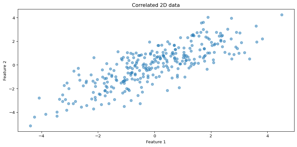
Figure 3: Correlated 2D data before PCA.

Example 1 — PCA directions & explained variance

from sklearn.decomposition import PCA

pca_2d = PCA(n_components=2)
X_pca = pca_2d.fit_transform(X)

print("Explained variance ratios:", pca_2d.explained_variance_ratio_)

# Plot original data and principal components as arrows
fig, ax = plt.subplots()
ax.scatter(X[:, 0], X[:, 1], alpha=0.4)

origin = X.mean(axis=0)

for length, vector in zip(pca_2d.explained_variance_ratio_, pca_2d.components_):
    # scale arrow length for visualization
    arrow = vector * length * 10  
    ax.arrow(origin[0], origin[1],
             arrow[0], arrow[1],
             head_width=0.2, color="black")

ax.set_xlabel("Feature 1")
ax.set_ylabel("Feature 2")
ax.set_title("PCA components on correlated 2D data")
ax.set_aspect("equal", adjustable="box")
plt.tight_layout()
plt.show()

Explained variance ratios: [0.90215352 0.09784648]

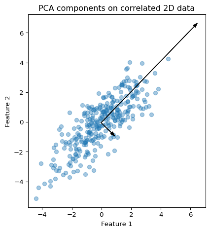
Figure 4: PCA components overlaid on the 2D data.

Example 1 — 1D reconstruction

# Keep only the first component
pca_1d = PCA(n_components=1)
X_1d = pca_1d.fit_transform(X)          # shape (n, 1)
X_recon = pca_1d.inverse_transform(X_1d)  # shape (n, 2)

fig, ax = plt.subplots()
ax.scatter(X[:, 0], X[:, 1], alpha=0.2, label="Original")
ax.scatter(X_recon[:, 0], X_recon[:, 1], alpha=0.6, label="Reconstructed (1D PCA)")

for i in range(0, len(X), 20):
    ax.plot([X[i, 0], X_recon[i, 0]],
            [X[i, 1], X_recon[i, 1]], ":", linewidth=0.5)

ax.set_xlabel("Feature 1")
ax.set_ylabel("Feature 2")
ax.set_title("PCA reconstruction from 1D")
ax.legend()
plt.tight_layout()
plt.show()

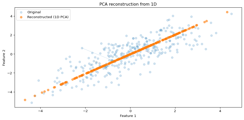
Figure 5: Projection onto the first principal component and reconstruction back to 2D.

Note

• Distances from original points to their reconstructions measure reconstruction error.
• Here, most structure is along the main diagonal; a 1D PCA captures it reasonably well.

💯 Example 2 — PCA for digits classification

Decision context:

• We want to classify handwritten digits (0–9).
• We care about:
  • Accuracy on a held-out test set.
  • Computational cost / training time.
  • Maybe interpretability of features.

Question:

• Does PCA as a pre-processing step help or hurt a simple classifier (e.g., logistic regression)?

We’ll compare:

1. Logistic regression on raw pixel features.
2. Logistic regression on PCA-compressed features with different dimensions \(k\).

from sklearn.datasets import load_digits
from sklearn.model_selection import train_test_split
from sklearn.preprocessing import StandardScaler
from sklearn.linear_model import LogisticRegression
from sklearn.decomposition import PCA
from sklearn.pipeline import Pipeline
from sklearn.metrics import accuracy_score
import pandas as pd

digits = load_digits()
X = digits.data
y = digits.target

X_train, X_test, y_train, y_test = train_test_split(
    X, y, test_size=0.3, random_state=3151, stratify=y
)

X_train.shape, X_test.shape

((1257, 64), (540, 64))

💯 Example 2 — baseline logistic regression

baseline_pipe = Pipeline(
    steps=[
        ("scaler", StandardScaler()),
        ("logreg", LogisticRegression(max_iter=1000, multi_class="auto"))
    ]
)

baseline_pipe.fit(X_train, y_train)

y_pred_base = baseline_pipe.predict(X_test)
acc_base = accuracy_score(y_test, y_pred_base)
print(f"Baseline test accuracy (no PCA): {acc_base:.3f}")

Baseline test accuracy (no PCA): 0.967

💯 Example 2 — PCA + logistic regression

results = []

for k in [5, 10, 20, 40, 64]:
    pipe = Pipeline(
        steps=[
            ("scaler", StandardScaler()),
            ("pca", PCA(n_components=k)),
            ("logreg", LogisticRegression(max_iter=1000, multi_class="auto"))
        ]
    )
    pipe.fit(X_train, y_train)
    y_pred = pipe.predict(X_test)
    acc = accuracy_score(y_test, y_pred)
    results.append({"n_components": k, "test_accuracy": acc})

results_df = pd.DataFrame(results)
results_df

	n_components	test_accuracy
0	5	0.803704
1	10	0.875926
2	20	0.942593
3	40	0.961111
4	64	0.966667

💯 Example 2 — accuracy vs dimension

fig, ax = plt.subplots()
ax.plot(results_df["n_components"], results_df["test_accuracy"], marker="o")
ax.axhline(acc_base, linestyle="--", label="Baseline (no PCA)")
ax.set_xlabel("Number of PCA components (k)")
ax.set_ylabel("Test accuracy")
ax.set_title("Digits classification: accuracy vs PCA dimension")
ax.legend()
plt.tight_layout()
plt.show()

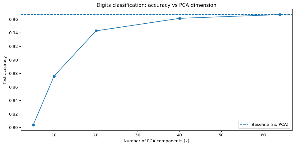
Figure 6

Design choices:

• Small \(k\) (e.g., 5, 10) = heavy compression:
  • May lose discriminative information → lower accuracy.
• Moderate \(k\) (e.g., 20, 40):
  • Often close to baseline or slightly better if noise is reduced.
• Large \(k\) (e.g., 64 out of 64):
  • Close to full-dimensional model; PCA buys little.

Warning

• PCA is not guaranteed to improve accuracy.
• It’s a tool for compression / visualization / denoising, and must be evaluated empirically for each task.

Final thoughts

Evaluation & quality checks for PCA

When you apply PCA in a pipeline, always ask:

1. What’s the goal?
   • Visualization? Compression? Speed? Regularization?
2. How will we evaluate success?
   • For compression:
     • Explained variance ratio (how much variance we keep).
   • For reconstruction:
     • Average reconstruction error \(\|X - \hat{X}\|_F^2 / n\).
   • For downstream tasks:
     • Task-specific metrics (accuracy, F1, etc.) on validation/test.
3. Where do we fit PCA?
   • Fit PCA on training data only (no leakage).
   • Apply the learned transform to validation/test sets.

👍️ Rule of thumb

• Choose the smallest \(k\) that:
  • Achieves acceptable explained variance (e.g., 90–95%), and
  • Does not significantly degrade downstream performance.

Curiosity: PCA and beyond

PCA and its descendants show up everywhere:

• Image compression & face recognition
  Classical eigenfaces use PCA on aligned face images to represent faces as linear combinations of principal components. Modern deep methods (e.g., FaceNet) learn nonlinear embeddings in a similar spirit (Turk and Pentland 1991; Schroff, Kalenichenko, and Philbin 2015).

• Genomics & population genetics
  PCA of genotype matrices reveals axes of ancestry and population structure, with a solid statistical treatment for large-scale genetics (Patterson, Price, and Reich 2006).

• Recommendation systems
  Matrix factorization models for user–item ratings are essentially low-rank (PCA/SVD-like) approximations of the rating matrix (Koren, Bell, and Volinsky 2009).

Connections & generalizations:

• Kernel PCA
  Nonlinear PCA in a feature space defined by a kernel, obtained by diagonalizing a kernel matrix rather than the covariance (Schölkopf, Smola, and Müller 1998).

• Deep autoencoders & VAEs
  Deep autoencoders and variational autoencoders learn nonlinear low-dimensional codes, extending PCA’s “bottleneck” idea to powerful generative models; recent work even blends kernel PCA with deep autoencoders for industrial fault detection (Hinton and Salakhutdinov 2006; Kingma and Welling 2014; Ren et al. 2024).

• Modern visualization methods (t-SNE, UMAP)
  t-SNE and UMAP focus on preserving local neighborhoods in low-dimensional embeddings and are standard tools for high-dimensional exploratory plots (e.g., single-cell RNA-seq, image features) (Maaten and Hinton 2008; McInnes, Healy, and Melville 2018).

Quick check

Q1 (MCQ).
Which of the following is closest to what PCA does?

A. Finds a linear classifier that minimizes misclassification error.
B. Finds directions that maximize the variance of the projected data, subject to orthogonality.
C. Finds directions that maximize classification accuracy using labels.
D. Finds directions that minimize the number of non-zero coefficients.

Q2 (short).
Why is it important to center the data before performing PCA?

Write a 1–2 sentence answer.

Q3 (numeric).

You run PCA and get the following explained variance ratios:

• PC1: 0.60
  
• PC2: 0.25
  
• PC3: 0.10
  
• PC4: 0.05

If you keep only the first two components, what fraction of the total variance do you retain?

Q4 (conceptual).

You have two features:

• height_cm in centimeters,
• income_dollars in dollars.

You apply PCA without scaling.
What is a likely issue, and how could you fix it?

References

Eckart, Carl, and Gale Young. 1936. “The Approximation of One Matrix by Another of Lower Rank.” Psychometrika 1 (3): 211–18. https://doi.org/10.1007/BF02288367.

Hinton, Geoffrey E., and Ruslan R. Salakhutdinov. 2006. “Reducing the Dimensionality of Data with Neural Networks.” Science 313 (5786): 504–7. https://doi.org/10.1126/science.1127647.

Kingma, Diederik P., and Max Welling. 2014. “Auto-Encoding Variational Bayes.” In Proceedings of the 2nd International Conference on Learning Representations (ICLR).

Koren, Yehuda, Robert Bell, and Chris Volinsky. 2009. “Matrix Factorization Techniques for Recommender Systems.” Computer 42 (8): 30–37. https://doi.org/10.1109/MC.2009.263.

Maaten, Laurens van der, and Geoffrey Hinton. 2008. “Visualizing Data Using t-SNE.” Journal of Machine Learning Research 9: 2579–2605.

McInnes, Leland, John Healy, and James Melville. 2018. “UMAP: Uniform Manifold Approximation and Projection for Dimension Reduction.” arXiv Preprint arXiv:1802.03426. https://arxiv.org/abs/1802.03426.

Patterson, Nick, Alkes L. Price, and David Reich. 2006. “Population Structure and Eigenanalysis.” PLOS Genetics 2 (12): e190. https://doi.org/10.1371/journal.pgen.0020190.

Ren, Zelin, Yuchen Jiang, Xuebing Yang, Yongqiang Tang, and Wensheng Zhang. 2024. “Learnable Faster Kernel-PCA for Nonlinear Fault Detection: Deep Autoencoder-Based Realization.” Journal of Industrial Information Integration 40: 100622. https://doi.org/10.1016/j.jii.2024.100622.

Schölkopf, Bernhard, Alexander Smola, and Klaus-Robert Müller. 1998. “Nonlinear Component Analysis as a Kernel Eigenvalue Problem.” Neural Computation 10 (5): 1299–319. https://doi.org/10.1162/089976698300017467.

Schroff, Florian, Dmitry Kalenichenko, and James Philbin. 2015. “FaceNet: A Unified Embedding for Face Recognition and Clustering.” In Proceedings of the IEEE Conference on Computer Vision and Pattern Recognition (CVPR), 815–23. https://doi.org/10.1109/CVPR.2015.7298682.

Turk, Matthew, and Alex Pentland. 1991. “Eigenfaces for Recognition.” Journal of Cognitive Neuroscience 3 (1): 71–86. https://doi.org/10.1162/jocn.1991.3.1.71.