M23: Feature engineering principles

CSCI 3151 — Foundations of Machine Learning

Frank Rudzicz

Today

  • Why features often matter as much as model choice
  • Common feature types & transformations
  • Good feature engineering practices
  • How to avoid data leakage
  • Using pipelines to keep everything honest & reproducible
  • Worked examples in Python:
    • Scaling & logistic regression on a real dataset
    • A tiny target-leakage demo

Learning outcomes

By the end of this module, you should be able to:

  1. Explain what “feature engineering” is and why it matters for generalization.
  2. Classify features (numeric, categorical, text, etc.) and choose suitable transformations.
  3. Diagnose potential data leakage in a feature set or preprocessing pipeline.
  4. Implement simple scikit-learn pipelines that combine preprocessing and models safely.
  5. Justify feature choices and transformations in terms of data-generating assumptions and evaluation goals.

What is a “feature”?

feature n.: A measurable property or attribute you feed into a model.

E.g.,

  • Tabular:
    • Age, income, number of logins last week
  • Image:
    • Pixel intensities, edges, 👉 CNN activations
  • Text:
    • Word counts, TF–IDF, 👉 embeddings
  • Graphs:
    • Node degree, centrality, learned node embeddings

Note

As indicated above (👉) a ‘feature’ can also be an internal representation from within a model, like a neural network, whose meaning is often indirect.

This can be confusing, since ‘feature’ can often refer to direct measures of the envioronment.

Feature engineering n.: Designing, transforming, and selecting these inputs so that:

  • They’re informative for the task
  • They respect the data-generating process
  • They are available at prediction time

Concept

Code
---
config:
  look: handDrawn
  handDrawnSeed: 3151
  theme: neutral
---
flowchart LR
  %% Nodes
  raw["Raw data<br>(database fields, logs, images, text)"]
  fe["Feature engineering<br>(clean, transform, encode,<br>aggregate)"]
  X["Feature matrix X"]
  model[Model]
  preds[Predictions]
  leakage[["Future labels / outcomes"]]

  %% Main pipeline
  raw --> fe
  fe  --> X
  X   --> model
  model --> preds

  %% Leakage arrow (dashed, labeled, red)
  leakage -.⚠ leakage.-> fe

  %% Style the leakage edge red
  %% Edge indices are zero-based in the order edges are declared above:
  %% 0: raw-->fe, 1: fe-->X, 2: X-->model, 3: model-->preds, 4: leakage-.->fe
  linkStyle 4 stroke:#ff0000,stroke-width:2px,color:#ff0000
---
config:
  look: handDrawn
  handDrawnSeed: 3151
  theme: neutral
---
flowchart LR
  %% Nodes
  raw["Raw data<br>(database fields, logs, images, text)"]
  fe["Feature engineering<br>(clean, transform, encode,<br>aggregate)"]
  X["Feature matrix X"]
  model[Model]
  preds[Predictions]
  leakage[["Future labels / outcomes"]]

  %% Main pipeline
  raw --> fe
  fe  --> X
  X   --> model
  model --> preds

  %% Leakage arrow (dashed, labeled, red)
  leakage -.⚠ leakage.-> fe

  %% Style the leakage edge red
  %% Edge indices are zero-based in the order edges are declared above:
  %% 0: raw-->fe, 1: fe-->X, 2: X-->model, 3: model-->preds, 4: leakage-.->fe
  linkStyle 4 stroke:#ff0000,stroke-width:2px,color:#ff0000
Feature engineering as writing code

You can often think of feature engineering as:

  • Starting from raw columns (text, timestamp, user_id, …)
  • Writing small, testable functions that map raw data to useful numbers
  • Wiring those functions into a reproducible pipeline so they run every time, consistently

A typical pattern:

def make_feature(df):
    # small, understandable transform
    return ...

df["new_feature"] = make_feature(df)

Tiny example — text polarity as a feature

Suppose we have a review_text column and want to predict whether a review is positive or negative.

One handcrafted feature:

  • For each review, compute average word polarity
def word_polarity(word):
    """Toy polarity function: positive, negative, or neutral word score."""
    if word in POSITIVE_WORDS:
        return 1.0
    elif word in NEGATIVE_WORDS:
        return -1.0
    else:
        return 0.0

def avg_polarity(text):
    words = tokenize(text.lower())
    scores = [word_polarity(w) for w in words]
    return float(np.mean(scores)) if scores else 0.0

df["avg_polarity"] = df["review_text"].apply(avg_polarity)
  • This is feature engineering:
    • You wrote code that turns raw text into a numeric signal.
    • A model can now combine avg_polarity with other features (e.g., length, user activity, etc.).

Custom transforms in a Pipeline (sketch)

Here is a sketch of how your custom feature functions might fit inside a pipeline.

from sklearn.preprocessing import FunctionTransformer
from sklearn.compose import ColumnTransformer
from sklearn.pipeline import Pipeline
from sklearn.linear_model import LogisticRegression
from sklearn.feature_extraction.text import CountVectorizer

numeric_cols = ["num_logins_7d", "account_age_days"]
text_col = "review_text"

def add_handcrafted_features(df):
    df = df.copy()
    df["avg_polarity"] = df[text_col].apply(avg_polarity)
    # you could add more handcrafted features here
    return df

feature_step = FunctionTransformer(add_handcrafted_features, validate=False)

preprocess = ColumnTransformer(
    transformers=[
        ("num", StandardScaler(), numeric_cols + ["avg_polarity"]),
        ("txt", CountVectorizer(min_df=5), text_col),
    ],
    remainder="drop",
)

pipe = Pipeline(
    steps=[
        ("handcrafted", feature_step),  # your Python feature code
        ("preprocess", preprocess),     # scaling + vectorization
        ("clf", LogisticRegression(max_iter=1000)),
    ]
)
  • All our little feature functions live inside one object.
  • Cross-validation and grid search can safely use the same pipe.

Why pipelines matter for feature engineering

Pipelines help to:

  • Prevent leakage:
    • Transforms are fit inside cross-validation folds, not on the whole dataset.
  • Keep code honest:
    • No forgotten “oh right, I scaled this column manually in a different cell”.
  • Make experiments reproducible:
    • The entire path from raw columns to predictions is encoded in one object.

We often start with ad-hoc code in a notebook and graduate to a pipeline once a pattern stabilizes.

Types of features (tabular focus)

  • Numeric (continuous)
    • Example: income, temperature, counts
    • Common transforms:
      • Standardization: \(x' = (x - \mu) / \sigma\)
      • Min–max scaling: \(x' = \frac{x - \min}{\max - \min}\)
      • Log transform: \(x' = \log(1 + x)\) for positive, skewed data
  • Categorical
    • Example: country, product type
    • Common transforms:
      • One-hot encoding
      • Ordinal encoding (only if the order is meaningful)
        • I.e., ‘binning’ (“age 0–18, 19–35, …”)
  • Binary flags
    • e.g., is_student, has_defaulted
  • Counts & rates
    • e.g., # purchases last month, click-through rate
    • Interactions like ratios \(\frac{x_1}{x_2}\) lets linear models approximate simple nonlinearities

Conceptual scaffold: distances & scale

Consider two observations with 2 features:

  • Height in meters, in \([1.5, 2.0]\)
  • Income in dollars, in \([10^3, 10^6]\)

Euclidean distance:

\[ d(\mathbf{x}, \mathbf{x}') = \sqrt{(h - h')^2 + (\text{income} - \text{income}')^2} \]

  • Without scaling, income dominates the distance.
  • After scaling both to zero mean and unit variance:
    • Height and income contribute more comparably.

Note

For distance-based kernels and models, feature scale effectively chooses which dimensions we care about.

❌ Anti-example: “Historical” feature that secretly sees the future

Suppose we’re predicting 30-day hospital readmission at the time of discharge.

You decide to add a patient-level feature:

patient_readmit_rate_30d
= fraction of this patient’s stays that are followed by a 30-day readmission

You compute it with something like:

patient_readmit_rate = (
    df.groupby("patient_id")["readmitted_30d"]
      .mean()
      .rename("patient_readmit_rate_30d")
)

df = df.merge(patient_readmit_rate, on="patient_id", how="left")

Looks reasonable, but:

  • This groupby uses all rows in the dataset, including:
    • The stay we’re trying to predict,
    • Future stays and their readmissions.
  • For an early admission, patient_readmit_rate_30d already “knows” how often this patient is readmitted later in the timeline.

This is target leakage:

  • During training, the model sees information that would not be known at prediction time.
  • Performance estimates become too optimistic.
  • A deployed model, which only knows a patient’s past stays, will perform much worse.

We want to train only on features that reflect information available up to the prediction time, not statistics computed over the full dataset.

🔬: scaling & regularization

For a linear model with L2 regularization:

\[ \hat{w} = \arg\min_w \;\; \frac{1}{n}\sum_{i=1}^n \ell(y_i, w^\top x_i) \;+\; \lambda \|w\|_2^2. \]

If we rescale a feature \(x_j' = s x_j\):

  • To keep the same predictor \(w^\top x = w_1 x_1 + \dots + w_j x_j + \dots\), we’d need:

\[ w_j' x_j' = w_j x_j \quad \Rightarrow \quad w_j' = \frac{w_j}{s}. \]

  • But the regularization term becomes:

\[ \lambda \|w'\|_2^2 = \lambda \left( \dots + \left(\frac{w_j}{s}\right)^2 + \dots \right). \]

So rescaling features effectively changes how strongly each feature is regularized.

Warning

In practice, always scale numeric features before L2/L1-regularized linear models, so the regularization strength is comparable across features.

Examples

Worked Example 1 — Dataset & baseline

Code
import numpy as np
import pandas as pd
import matplotlib.pyplot as plt

from sklearn.datasets import load_breast_cancer, make_classification
from sklearn.model_selection import train_test_split, cross_val_score
from sklearn.preprocessing import StandardScaler
from sklearn.linear_model import LogisticRegression
from sklearn.pipeline import Pipeline

🥅 Goal: see how feature scaling interacts with logistic regression.

We’ll use the breast cancer dataset from scikit-learn:

Code
data = load_breast_cancer()
X = data.data
y = data.target
feature_names = data.feature_names

df = pd.DataFrame(X, columns=feature_names)
df["target"] = y
df.head()
mean radius mean texture mean perimeter mean area mean smoothness mean compactness mean concavity mean concave points mean symmetry mean fractal dimension ... worst texture worst perimeter worst area worst smoothness worst compactness worst concavity worst concave points worst symmetry worst fractal dimension target
0 17.99 10.38 122.80 1001.0 0.11840 0.27760 0.3001 0.14710 0.2419 0.07871 ... 17.33 184.60 2019.0 0.1622 0.6656 0.7119 0.2654 0.4601 0.11890 0
1 20.57 17.77 132.90 1326.0 0.08474 0.07864 0.0869 0.07017 0.1812 0.05667 ... 23.41 158.80 1956.0 0.1238 0.1866 0.2416 0.1860 0.2750 0.08902 0
2 19.69 21.25 130.00 1203.0 0.10960 0.15990 0.1974 0.12790 0.2069 0.05999 ... 25.53 152.50 1709.0 0.1444 0.4245 0.4504 0.2430 0.3613 0.08758 0
3 11.42 20.38 77.58 386.1 0.14250 0.28390 0.2414 0.10520 0.2597 0.09744 ... 26.50 98.87 567.7 0.2098 0.8663 0.6869 0.2575 0.6638 0.17300 0
4 20.29 14.34 135.10 1297.0 0.10030 0.13280 0.1980 0.10430 0.1809 0.05883 ... 16.67 152.20 1575.0 0.1374 0.2050 0.4000 0.1625 0.2364 0.07678 0

5 rows × 31 columns

  • Each row: a tumor
  • Features: cell measurements
  • Target: malignant vs benign

Example 1 — Unscaled vs scaled logistic regression

Code
log_reg_plain = LogisticRegression(max_iter=1000)

pipe_scaled = Pipeline(
    [
        ("scaler", StandardScaler()),
        ("logreg", LogisticRegression(max_iter=1000)),
    ]
)

scores_plain = cross_val_score(log_reg_plain, X, y, cv=5)
scores_scaled = cross_val_score(pipe_scaled, X, y, cv=5)

results = pd.DataFrame(
    {
        "setting": ["unscaled", "with_standard_scaler"],
        "cv_mean_accuracy": [scores_plain.mean(), scores_scaled.mean()],
        "cv_std": [scores_plain.std(), scores_scaled.std()],
    }
)

results
setting cv_mean_accuracy cv_std
0 unscaled 0.952569 0.014200
1 with_standard_scaler 0.980686 0.006539

Design choices:

  • Same model, same CV split
  • Only difference: feature scaling
  • Notice how scaling usually improves stability and often performance for linear models.

Example 1: Feature importance view

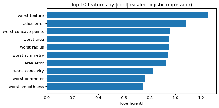
Let’s inspect the magnitude of learned coefficients after scaling.

  • Here, logreg = pipe_scaled.named_steps["logreg"] pulls out the fitted logistic regression model from the pipeline, and
  • coefs = logreg.coef_[0] reads its coefficient vector, whose magnitudes are a simple measure of feature importance (because we scaled the inputs).
Code
X_train, X_test, y_train, y_test = train_test_split(
    X, y, test_size=0.2, stratify=y, random_state=42
)

pipe_scaled.fit(X_train, y_train)
logreg = pipe_scaled.named_steps["logreg"]

coefs = logreg.coef_[0]
coef_df = (
    pd.DataFrame({"feature": feature_names, "abs_coef": np.abs(coefs)})
    .sort_values("abs_coef", ascending=False)
    .head(10)
)
coef_df
feature abs_coef
21 worst texture 1.255088
10 radius error 1.082965
27 worst concave points 0.953686
23 worst area 0.947756
20 worst radius 0.947616
28 worst symmetry 0.939181
13 area error 0.929104
26 worst concavity 0.823151
22 worst perimeter 0.763220
24 worst smoothness 0.746625

This table shows the top 10 features by absolute coefficient value.

Example 1: Coefficient magnitudes

Code
plt.figure(figsize=(8, 4))
plt.barh(coef_df["feature"], coef_df["abs_coef"])
plt.gca().invert_yaxis()
plt.xlabel("|coefficient|")
plt.title("Top 10 features by |coef| (scaled logistic regression)")
plt.tight_layout()
plt.show()
Figure 1: Top 10 features by |coefficient| for scaled logistic regression.

Interpretation:

  • After scaling, comparing coefficient magnitudes is meaningful:
    • larger |coef| → stronger influence on the log-odds (keeping others fixed)
  • Without scaling, raw coefficient sizes mix effect size with unit choices.

Example 1: Design subtleties

🤔 Key observations:

  • Even simple models like logistic regression rely heavily on feature scaling.
  • Coefficient-based interpretation only makes sense if:
    • Features are on comparable scales, and
    • The model is appropriately regularized.

Design questions to ask:

  • Do my features have wildly different ranges?
  • Am I comparing models fairly (same preprocessing, same splits)?
  • Does my interpretation depend on units?

Example 2: Target leakage toy demo

🥅 Goal: show how “too good to be true” performance often means leakage.

We’ll:

  1. Make a simple synthetic classification dataset.
  2. Train a logistic regression model on:
    • Original features only
    • Original features plus a leaky feature that encodes the label
Code
X_base, y_base = make_classification(
    n_samples=2000,
    n_features=5,
    n_informative=3,
    n_redundant=0,
    n_clusters_per_class=2,
    random_state=42,
)

base_model = LogisticRegression(max_iter=1000)

scores_base = cross_val_score(base_model, X_base, y_base, cv=5)
scores_base.mean(), scores_base.std()
(np.float64(0.9129999999999999), np.float64(0.005567764362830011))

The mean/std here give a reasonable baseline.

Example 2: Adding a leaky feature

Now we’ll add a “feature” that is literally the label:

Code
# Append the true label as an extra feature (this is NOT allowed in reality!)
X_leaky = np.column_stack([X_base, y_base])

scores_leaky = cross_val_score(base_model, X_leaky, y_base, cv=5)

results_leak = pd.DataFrame(
    {
        "features": ["original", "with_leaky_label_feature"],
        "cv_mean_accuracy": [scores_base.mean(), scores_leaky.mean()],
        "cv_std": [scores_base.std(), scores_leaky.std()],
    }
)

results_leak
features cv_mean_accuracy cv_std
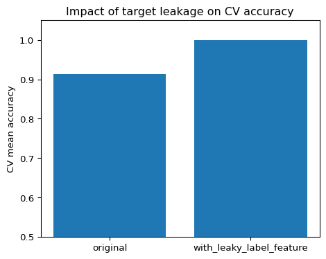
0 original 0.913 0.005568
1 with_leaky_label_feature 1.000 0.000000

The table should show much higher accuracy when we leak the label.

Example 2: Leakage visualization

Code
plt.figure(figsize=(5, 4))
plt.bar(results_leak["features"], results_leak["cv_mean_accuracy"])
plt.ylim(0.5, 1.05)
plt.ylabel("CV mean accuracy")
plt.title("Impact of target leakage on CV accuracy")
plt.tight_layout()
plt.show()
Figure 2: Target leakage can make cross-validation accuracy look unrealistically high.

Leakage patterns out for which to watch

  • In real data, leakage is usually more subtle:
    • “Aggregated” features computed with knowledge of the outcome
      • E.g., A clinical assessment of cognition as input to a dementia detector
  • Any surprisingly high performance deserves a leakage investigation.
    • Features with perfect or near-perfect correlation with the label
    • Features computed using:
      • Future events (after the label is realized)
      • Global statistics that mix train & test (e.g., using all data to compute per-group label rates)
    • Preprocessing done before the train/test split that depends on labels

Final thoughts

Pipelines to reduce mistakes

Instead of:

# BAD STYLE
X_train, X_test, y_train, y_test = train_test_split(X, y)
scaler = StandardScaler()
X_train_scaled = scaler.fit_transform(X_train)
X_test_scaled = scaler.transform(X_test)  # easy to forget & misuse later
model = LogisticRegression().fit(X_train_scaled, y_train)

Prefer:

pipe = Pipeline(
    [
        ("scaler", StandardScaler()),
        ("logreg", LogisticRegression(max_iter=1000)),
    ]
)

pipe.fit(X_train, y_train)
pipe.score(X_test, y_test)  # safely applies scaler + model
  • All preprocessing steps live inside the pipeline.
  • Cross-validation & grid search automatically keep things in sync.

Ethics & risks in feature choices

Feature engineering can introduce ethical issues:

  • Using sensitive attributes:
    • Race, gender, disability status, etc.
  • Proxies for sensitive attributes:
    • Postal code, income, name patterns

Potential mitigations (at this course level):

  • Document feature choices and justify each one.
  • Check performance across subgroups when possible.
  • Consider removing or carefully handling features that encode structural bias.
  • Remember: a highly predictive feature is not always acceptable to use.

Curiosity: where this shows up in practice

  • Feature stores in industry:
    • Centralized, versioned feature definitions shared across teams.
  • Automated feature engineering:
    • Tools that search over transforms, interactions, and aggregations.
  • Deep learning:
    • Many architectures perform representation learning → automatic feature construction.
  • Explainability tools:
    • Feature importance, SHAP values, counterfactual explanations, etc.
    • Help debug whether learned features align with domain understanding.

Feature engineering connects hand-crafted features with learned representations later in the course.

Quick checks

  1. A positive-valued feature (e.g., income) is heavily right-skewed with a few extreme outliers.
    Which transform is usually most appropriate to try first?

    A. No transform
    B. Standardization only
    C. Log transform (e.g., log1p)
    D. One-hot encoding

  2. True or False:
    “Tree-based models (like random forests) always require standardizing numeric features.”

  3. Which scenario is the clearest example of data leakage?

    A. Using age and gender to predict heart disease risk.
    B. Using a lab test result that becomes available two days after the diagnosis time you want to predict.
    C. Standardizing features using StandardScaler.
    D. Using one-hot encoding for country.

  4. Short answer:

    You’re predicting whether a user will churn next month. You create a feature that is “number of support tickets opened in the month after churn.”
    Briefly explain why this is problematic.

Wrap-up

Key messages:

  • Features are the language your model uses to understand the world.
  • Good feature engineering is:
    • Grounded in the data-generating process
    • Careful about scale, leakage, and availability
    • Encoded in pipelines, not in ad-hoc scripts
  • These tools & habits set you up for:
    • Data augmentation (M24)
    • Dimensionality reduction and learned representations in later modules
