M17: Optimization basics – gradient descent & variants
CSCI 3151 — Foundations of Machine Learning
Frank Rudzicz
Learning outcomes
By the end of this module, you should be able to:
- Explain the role of optimization in the ML pipeline and its relationship to empirical risk minimization.
- Derive and implement basic gradient descent for simple regression objectives.
- Distinguish and compare batch gradient descent, stochastic gradient descent (SGD), and mini-batch SGD in terms of speed and noise.
- Tune and diagnose learning rate and batch size using loss curves and simple metrics.
- Describe the intuition behind momentum and adaptive methods (e.g., Adam) and when they are useful.
Conceptual scaffold
Where does optimization fit?
Recall the supervised learning pipeline:
- Choose a model family \(f_w(x)\) (hypothesis space).
- Choose a loss (and possibly a regularizer).
- Optimize the empirical risk (plus penalty) to find good parameters \(w\).
- Evaluate and deploy.
Optimization is Step 3:
- We want \(w^* = \underset{w}{\text{arg min}}\, J(w)\) where \[ J(w) = \hat{R}(w) + \lambda \Omega(w). \]
- For some models (e.g., ordinary least squares), we have closed-form solutions.
- For many others (logistic regression, neural networks, complex regularizers), we rely on iterative optimization algorithms.
Tradeoffs in optimization
Conceptual tradeoffs:
- Accuracy of each step vs compute per step.
- Global view of the loss surface vs local, noisy updates.
- Theoretical guarantees vs practical performance on finite data.
Gradient-based methods are a sweet spot:
- They use local slope information (the gradient) to move downhill.
- Can scale to large datasets and high dimensions with SGD / mini-batching.
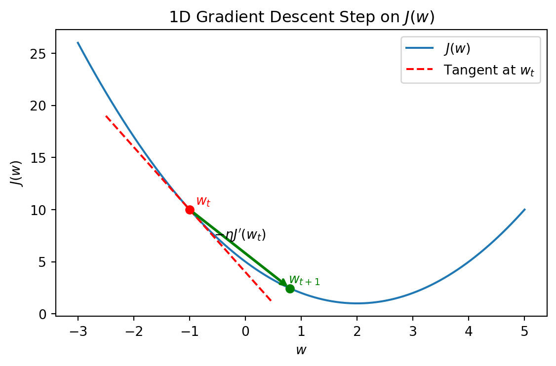
Gradient descent: 1D intuition
Consider a smooth function \(J(w)\) of a single parameter \(w\).
- The gradient (derivative) \(J'(w)\) tells us:
- Sign: which direction increases / decreases the function.
- Magnitude: how steep the slope is.
Gradient descent update (1D):
\[ w_{t+1} = w_t - \eta \, J'(w_t), \]
where \(\eta > 0\) is the learning rate (step size).
Intuition:
- If \(J'(w_t) > 0\), the function is increasing → move left (decrease \(w\)).
- If \(J'(w_t) < 0\), the function is decreasing → move right (increase \(w\)).
- The larger \(|J'(w_t)|\), the larger the step — scaled by \(\eta\).
Gradient descent in multiple dimensions
In \(d\) dimensions with parameter vector \(w \in \mathbb{R}^d\), we use the gradient vector
\[ \nabla_w J(w) = \left( \frac{\partial J}{\partial w_1}, \dots, \frac{\partial J}{\partial w_d} \right). \]
Batch gradient descent update:
\[ w_{t+1} = w_t - \eta \, \nabla_w J(w_t). \]
- Each iteration uses the full training set to compute the gradient.
- For large datasets, this can be expensive per step but gives a relatively stable direction.
Convergence intuition
For a simple convex, smooth function, gradient descent with a small enough learning rate:
- Decreases the objective almost every step.
- Converges to a (possibly global) minimum.
For this course, remember:
- Too large \(\eta\) → instability or divergence.
- Too small \(\eta\) → painfully slow convergence.
- We often tune \(\eta\) empirically using simple loss vs iteration plots.
Worked derivation: GD on a 1D quadratic
Consider:
\[ J(w) = \frac{1}{2} a w^2, \quad a > 0. \]
where \(a > 0\) is a constant controlling the curvature.
- Gradient: \(J'(w) = a w\).
- Gradient descent update:
\[ w_{t+1} = w_t - \eta a w_t = (1 - \eta a) w_t. \]
Iterating:
\[ w_t = (1 - \eta a )^t w_0. \]
Convergence condition (sketch):
- We need \(\lvert 1 - \eta a \rvert < 1\) in magnitude so that \(w_t \to 0\).
- That is:
\[ -1 < 1 - \eta a < 1 \quad \Rightarrow \quad 0 < \eta a < 2 \quad \Rightarrow \quad 0 < \eta < 2/a. \]
Takeaways:
- There is a range of stable learning rates.
- Within that range, smaller \(\eta\) is safer but slower.
You can think of many ML losses as generalized quadratics near an optimum, so similar intuition applies.
Stochastic gradient descent (SGD) & mini-batching
For an average loss over data:
\[ J(w) = \frac{1}{n} \sum_{i=1}^n \ell_i(w), \]
batch gradient descent uses the full sum each step.
Stochastic gradient descent (SGD)
- At each step \(t\), randomly pick an index \(i_t\) and update:
\[ w_{t+1} = w_t - \eta \, \nabla_w \ell_{i_t}(w_t). \]
Characteristics:
- Much cheaper per step (uses 1 example).
- Updates are noisy, but can explore the loss surface better.
- Often generalizes well in practice, especially in deep learning.
Mini-batch SGD
- Use a small batch \(B_t\) (e.g., 32 or 128 examples):
\[ g_t = \frac{1}{\lvert B_t \rvert} \sum_{i \in B_t} \nabla_w \ell_i(w_t), \quad w_{t+1} = w_t - \eta g_t. \]
Tradeoffs:
- Batch size \(= 1\): noisier but very cheap.
- Batch size \(= n\): full batch GD.
- In practice, mini-batch SGD is the standard.
Variants (high level)
Momentum (very high level)
- 💡 Idea: keep a running velocity that points in a direction where past gradients have consistently pushed us.
\[ v_{t+1} = \beta v_t + \nabla J(w_t), \quad w_{t+1} = w_t - \eta v_{t+1}, \]
where: \(\eta\) is the learning rate and \(\beta \in [0, 1)\) is the momentum parameter.
- 🤔 Intuition:
- In narrow valleys, vanilla GD can zig–zag.
- Momentum accumulates consistent gradient directions, smoothing the path and often converging faster.
- 📚 Further reading (optional):
We’ll visualize this on a simple “elongated bowl” loss.
Momentum
Adaptive methods (e.g., Adam, RMSProp)
Goal: use per-parameter learning rates that adapt over time.
Examples:
- AdaGrad (Duchi, Hazan, and Singer 2011): accumulates squared gradients, shrinking the step size more for frequently-updated parameters.
- RMSProp (Tieleman and Hinton 2012): “leaky” AdaGrad with an exponential moving average of squared gradients.
- Adam (Kingma and Ba 2015): roughly RMSProp + momentum with bias-corrected first and second moment estimates.
Adam update (elementwise):
\[ m_{t} = \beta_1 m_{t-1} + (1 - \beta_1) g_t, \quad v_{t} = \beta_2 v_{t-1} + (1 - \beta_2) g_t^2 \]
\[ \hat m_t = \frac{m_t}{1 - \beta_1^t}, \quad \hat v_t = \frac{v_t}{1 - \beta_2^t}, \quad w_{t+1} = w_t - \eta \frac{\hat m_t}{\sqrt{\hat v_t} + \varepsilon}. \]
📝 Notes:
- Very popular in deep learning; often “just works” with default hyperparameters.
- But convergence theory is subtle: Reddi, Kale, and Kumar (2018) showed Adam can fail to converge on simple convex problems and propose AMSGrad as a fix.
❌ Anti-example: bad learning rates
Too large learning rate
- Loss bounces around or diverges.
- Parameters can shoot off to huge magnitudes.
- Training accuracy may be erratic; validation loss never stabilizes.
Too small learning rate
- Loss decreases very slowly.
- Training may appear “stuck” far from optimum.
- You might mistake slow progress for a fundamental modeling problem.
Diagnosis tool: plot loss vs iteration (and sometimes gradient norm):
- Diverging / exploding → try smaller \(\eta\).
- Very flat / slow → try larger \(\eta\) (or momentum).
Examples
Worked example 1: linear regression with gradient descent
We’ll fit a simple line \(y \approx w_0 + w_1 x\) with explicit gradient descent, and compare to the closed-form solution.
Code
import numpy as np
import pandas as pd
import matplotlib.pyplot as plt

rng = np.random.default_rng(3151)

# Generate synthetic data: y = 3x + 1 + noise
n = 80
X = rng.uniform(-2, 2, size=(n, 1))
true_w0, true_w1 = 1.0, 3.0
noise = rng.normal(0, 0.8, size=n)
y = true_w0 + true_w1 * X.ravel() + noise

# Add bias column for w0
X_design = np.c_[np.ones_like(X), X]  # shape (n, 2)

X[:5], y[:5]
(array([[ 0.13866131],
[-1.7206137 ],
[ 0.58167979],
[-1.75712451],
[ 1.86113116]]),
array([ 1.98278139, -4.34254563, 2.87329754, -4.45654002, 5.22714618]))Implement batch gradient descent
Code
def mse_loss(w, X, y):
    # Mean squared error loss for linear regression.
    y_pred = X @ w
    return np.mean((y - y_pred) ** 2)

def mse_grad(w, X, y):
    # Gradient of MSE loss wrt w.
    y_pred = X @ w
    return -2.0 * (X.T @ (y - y_pred)) / len(y)

# Initialize
w = np.zeros(2)
eta = 0.05
num_iters = 200

loss_history = []

for t in range(num_iters):
    loss = mse_loss(w, X_design, y)
    loss_history.append(loss)
    g = mse_grad(w, X_design, y)
    w = w - eta * g

w, loss_history[-1]
(array([1.04384639, 3.0594615 ]), 0.616479536206361)Visualize convergence & final fit
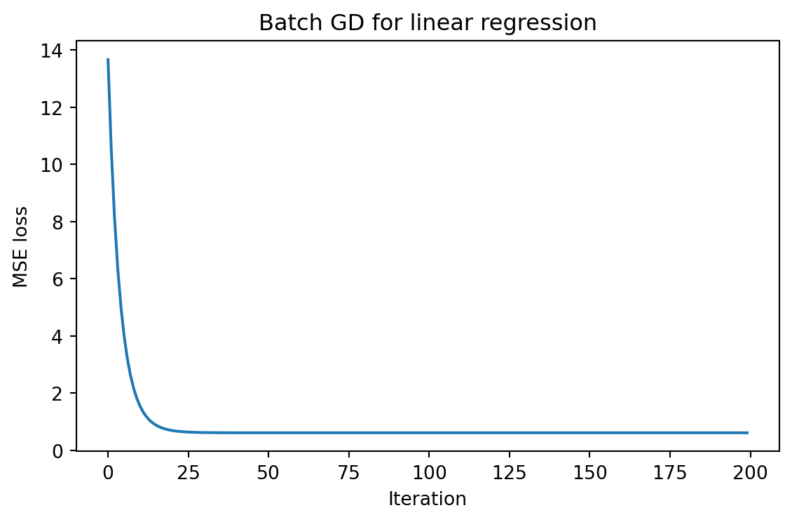
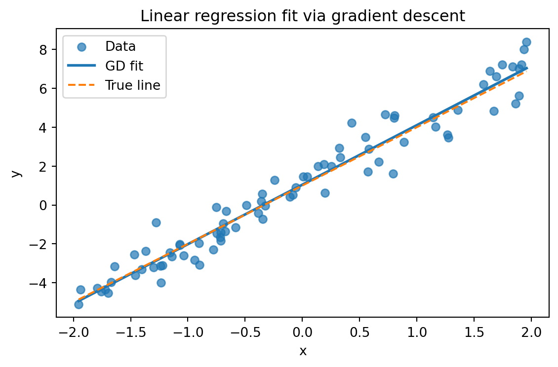
Design choices & subtleties:
- We used a single learning rate and fixed number of iterations.
- With a too-large \(\eta\), the loss would diverge; with too-small, it would flatten slowly.
- In higher dimensions, behaviour is similar but harder to visualize.
Worked example 2: logistic regression with mini-batch SGD
We’ll implement a simple mini-batch SGD optimizer for logistic regression.
Code
from sklearn.datasets import make_classification
from sklearn.metrics import accuracy_score

# Synthetic binary classification
X_cls, y_cls = make_classification(
    n_samples=800,
    n_features=4,
    n_informative=3,
    n_redundant=0,
    random_state=3151,
)

# Add bias column
X_cls_design = np.c_[np.ones((X_cls.shape[0], 1)), X_cls]

# Train/test split
from sklearn.model_selection import train_test_split

X_train, X_test, y_train, y_test = train_test_split(
    X_cls_design, y_cls, test_size=0.3, random_state=3151
)

X_train.shape, X_test.shape
((560, 5), (240, 5))Implement mini-batch SGD for logistic loss
Code
def sigmoid(z):
    return 1.0 / (1.0 + np.exp(-z))

def logistic_loss_and_grad(w, X, y):
    # Negative log-likelihood (average) for logistic regression and its gradient.
    scores = X @ w
    probs = sigmoid(scores)
    # Binary cross-entropy loss
    eps = 1e-12
    loss = -np.mean(y * np.log(probs + eps) + (1 - y) * np.log(1 - probs + eps))
    grad = X.T @ (probs - y) / len(y)
    return loss, grad

def sgd_logistic(X, y, eta=0.1, batch_size=32, num_epochs=20, rng=None):
    rng = np.random.default_rng(rng)
    n, d = X.shape
    w = np.zeros(d)
    history = []

    for epoch in range(num_epochs):
        # Shuffle indices each epoch
        indices = rng.permutation(n)
        for start in range(0, n, batch_size):
            batch_idx = indices[start:start + batch_size]
            X_batch = X[batch_idx]
            y_batch = y[batch_idx]
            loss, grad = logistic_loss_and_grad(w, X_batch, y_batch)
            w = w - eta * grad
            history.append(loss)
    return w, history

w_sgd, loss_hist_sgd = sgd_logistic(
    X_train, y_train,
    eta=0.1,
    batch_size=32,
    num_epochs=30,
    rng=3151,
)

len(loss_hist_sgd), loss_hist_sgd[:5]
(540,
[0.6931471805579453,
0.6848241436460908,
0.673225537662632,
0.6782243265743305,
0.6727666003601709])Evaluate and visualize SGD behaviour
Code
# Loss vs update step
plt.figure(figsize=(6, 4))
plt.plot(loss_hist_sgd)
plt.xlabel("Update step")
plt.ylabel("Mini-batch loss")
plt.title("Mini-batch SGD for logistic regression")
plt.tight_layout()
plt.show()

# Train and test accuracy
def predict_logistic(w, X):
    return (sigmoid(X @ w) >= 0.5).astype(int)

y_train_pred = predict_logistic(w_sgd, X_train)
y_test_pred = predict_logistic(w_sgd, X_test)

train_acc = accuracy_score(y_train, y_train_pred)
test_acc = accuracy_score(y_test, y_test_pred)

train_acc, test_acc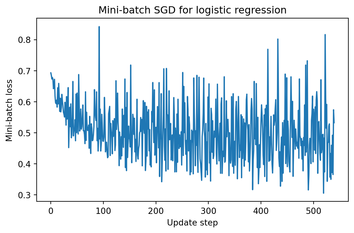
Discussion:
- Loss is noisy (because of mini-batches) but should trend downward.
- Try different
etaandbatch_sizevalues:- See when training diverges vs converges.
- Observe tradeoffs between noise and speed.
Evaluation & quality checks
When using gradient-based optimization, we should monitor:
- Training loss vs iteration:
- Detect divergence, plateaus, or oscillations.
- Validation loss vs iteration:
- Detect overfitting (val loss starts increasing).
- Suggests early stopping or stronger regularization.
- Simple metrics (accuracy, MSE) on train vs validation:
- Ensure optimization is actually improving model performance, not just fitting noise.
- Runtime & iterations:
- If optimization is very slow, reconsider:
- Learning rate, batch size, or using an adaptive method.
- If optimization is very slow, reconsider:
These checks connect directly back to evaluation & bias–variance and regularization modules.
Ethics & risks
Although optimization sounds purely technical, there are risks:
- Silent failure:
- If training diverges or gets stuck but you only look at final metrics, you might unknowingly deploy a poorly optimized model.
- Reproducibility:
- SGD uses randomness (shuffling, initialization).
- Without fixing seeds or documenting hyperparameters, results may be hard to reproduce.
SGD / Adam in practice (PyTorch)
So far: we wrote updates like
\[ w_{t+1} = w_t - \eta \nabla J(w_t) \quad\text{and}\quad \text{Adam updates with } m_t, v_t. \]
In practice, you’ll usually see these wrapped in a library optimizer.
import torch
import torch.nn as nn

model = MyNeuralNet()                 # your model
criterion = nn.CrossEntropyLoss()     # or MSELoss, etc.

# Option 1: SGD + momentum
sgd_opt = torch.optim.SGD(
    model.parameters(),
    lr=0.1,
    momentum=0.9,       # like "heavy-ball" momentum
    weight_decay=1e-4,  # L2 regularization
)

# Option 2: Adam
adam_opt = torch.optim.Adam(
    model.parameters(),
    lr=1e-3,            # often smaller than SGD lr
    weight_decay=1e-4,  # decoupled "AdamW" variant is common
)

# Typical training loop (same structure for both)
optimizer = adam_opt   # or sgd_opt

for X_batch, y_batch in train_loader:
    optimizer.zero_grad()          # reset gradients
    y_pred = model(X_batch)        # forward pass
    loss = criterion(y_pred, y_batch)
    loss.backward()                # compute gradients
optimizer.step() # apply update rule- Things to notice:
- You never write the update \(w_{t+1} = \dots\) by hand.
- You choose:
- optimizer class (SGD, Adam, …),
- lr (learning rate),
- optional knobs like momentum, betas, weight_decay.
- Under the hood, PyTorch is implementing the update rules we just derived/outlined.
- See 🔗PyTorch documentation
Note
In most real projects, “which optimizer? which lr?” is tuned by experiments + experience, not by pure theory.
Curiosity / broader connections
- Modern deep learning often involves hundreds of millions of parameters, trained via SGD or Adam.
- Research questions you might see later:
- Why does SGD generalize so well in overparameterized regimes?
- What implicit regularization does plain gradient descent provide?
- How do different optimizers affect robustness and fairness?
This module gives you the foundational tools to start thinking about such questions.
Quick check
(MCQ) Which of the following is not a typical reason to prefer mini-batch SGD over full-batch gradient descent?
A. Lower memory usage per update
B. Faster updates per unit of data processed
C. Ability to compute the exact gradient at each step
D. Better scalability to large datasets(MCQ) For the 1D quadratic \(J(w) = \frac{1}{2} a w^2\) with \(a > 0\), which range of learning rates \(\eta\) guarantees convergence of gradient descent?
A. \(\eta > 2/a\)
B. \(0 < \eta < 2/a\)
C. \(0 < \eta < a/2\)
D. Any \(\eta > 0\)(Concept) Briefly explain the difference between batch gradient descent and stochastic gradient descent in terms of how the gradient is computed.
(Numeric) Suppose we run gradient descent on \(J(w) = w^2\) with learning rate \(\eta = 0.25\) and initial value \(w_0 = 4\).
Compute \(w_1\) and \(w_2\).
References
Duchi, John, Elad Hazan, and Yoram Singer. 2011. “Adaptive Subgradient Methods for Online Learning and Stochastic Optimization.” Journal of Machine Learning Research 12: 2121–59.
Kingma, Diederik P., and Jimmy Ba. 2015. “Adam: A Method for Stochastic Optimization.” In International Conference on Learning Representations (ICLR).
Nesterov, Yurii. 1983. “A Method of Solving a Convex Programming Problem with Convergence Rate \(O(1/k^2)\).” Soviet Mathematics Doklady 27 (2): 372–76.
Polyak, Boris T. 1964. “Some Methods of Speeding up the Convergence of Iteration Methods.” USSR Computational Mathematics and Mathematical Physics 4 (5): 1–17.
Reddi, Sashank J., Satyen Kale, and Sanjiv Kumar. 2018. “On the Convergence of Adam and Beyond.” In International Conference on Learning Representations (ICLR).
Sutskever, Ilya, James Martens, George E. Dahl, and Geoffrey E. Hinton. 2013. “On the Importance of Initialization and Momentum in Deep Learning.” In Proceedings of the 30th International Conference on Machine Learning (ICML), 1139–47.
Tieleman, Tijmen, and Geoffrey Hinton. 2012. “Lecture 6.5—RMSProp: Divide the Gradient by a Running Average of Its Recent Magnitude.” Coursera: Neural Networks for Machine Learning.
