M16: Regularization - L2, L1, and Beyond

CSCI 3151 — Foundations of Machine Learning

Frank Rudzicz

Module context

  • Cluster: C05 — Regularization & Optimization Basics

Narrative position

  • This module is the bridge between:
    • Evaluation & bias–variance (how we know a model is good), and
    • Optimization (how we actually fit models).

Here we focus on how to intentionally control model capacity to improve generalization.

Learning outcomes

After this module, you should be able to:

  1. Explain what regularization is and how it relates to model capacity and overfitting.
  2. Write down and interpret regularized objectives with L2, L1, and elastic net penalties.
  3. Implement and compare L2- and L1-regularized models in Python on small datasets.
  4. Analyze how regularization strength affects training vs. validation performance and learning curves.
  5. Justify practical choices of regularization (type + strength) for different decision contexts.

Motivation: when good training loss is bad

  • You fit a complex model; training error is almost zero.
  • But on validation data:
    • Accuracy drops, or
    • Loss explodes, or
    • Predictions are unstable across splits.

Key tension

  • We want models that generalize, not just memorize.
  • Raw training loss does not penalize “too much flexibility”.

👉 Regularization = “discipline” for models

  • Explicitly discourages overly complex solutions.
  • Trades a bit of bias for reduced variance (see M14).

Conceptual scaffold

Capacity

  • Informally: how “flexible” a model is.
  • High capacity:
    • Deep nets with 100B parameters.
    • High-degree polynomials.
  • Low capacity:
    • Simple linear models with few features.

Note

What constitutes ‘high’ or ‘low’ is very related to context. Sometimes, even a few dozen paremeters are ‘too much’; other times, 70B parameters are ‘too few’.

Regularization (conceptual)

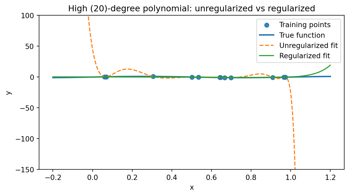
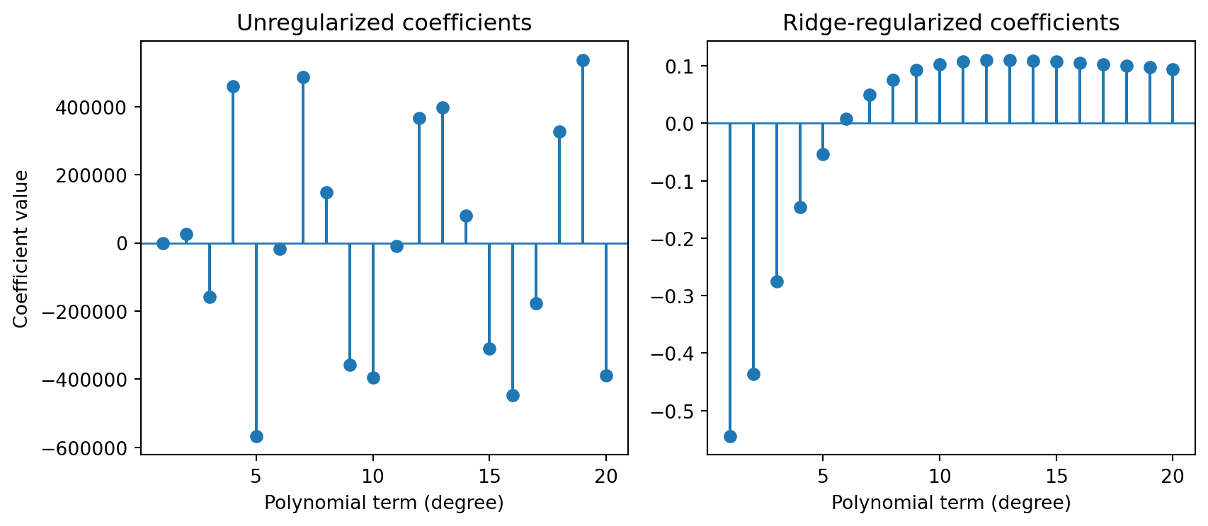
Regularization adds an explicit preference for “simple” parameter settings to the training objective.

Warning

This doesn’t mean simple as in fewer parameters. It means making the parameters you do have less likely to fluctuate wildly.

  • Instead of minimizing:

\[ \frac{1}{n} \sum_{i=1}^n \ell(y_i, f_\mathbf{w}(x_i)) \]

  • We minimize:

\[ \frac{1}{n} \sum_{i=1}^n \ell(y_i, f_\mathbf{w}(x_i)) + \color{blue}{ \lambda \, \Omega(\mathbf{w})} \]

where \(\ell\) is the loss, \(\Omega(\mathbf{w})\) is a penalty on parameters, and \(\lambda \ge 0\) controls regularization strength.

Capacity vs data

Code
import numpy as np
import plotly.graph_objects as go

# "Capacity" axis: 0 = very simple, 1 = very flexible
capacity = np.linspace(0.0, 1.0, 200)

# Toy curves (just for visualization)
gen_error = 0.35 * (capacity - 0.55) ** 2 + 0.2   # U-shaped generalization error
train_error = 0.5 - 0.35 * capacity               # monotonically decreasing training error

sweet_spot = 0.55
too_flexible = 0.9

fig = go.Figure()

# Generalization error
fig.add_trace(
    go.Scatter(
        x=capacity,
        y=gen_error,
        mode="lines",
        name="Expected generalization error",
    )
)

# Training error (for context)
fig.add_trace(
    go.Scatter(
        x=capacity,
        y=train_error,
        mode="lines",
        name="Training error",
        line=dict(dash="dash")
    )
)

# Sweet spot marker
fig.add_vline(
    x=sweet_spot,
    line=dict(width=2),
    annotation_text="sweet spot",
    annotation_position="top"
)

# Arrow: regularization pushing from high capacity back toward sweet spot
fig.add_annotation(
    x=too_flexible,
    y=float(gen_error[capacity.argmax()]),  # just park it near the right
    ax=sweet_spot + 0.02,
    ay=float(gen_error[np.abs(capacity - sweet_spot).argmin()]) + 0.03,
    text="↑ λ (stronger regularization)",
    showarrow=True,
    arrowhead=2
)

fig.update_layout(
    xaxis_title="Model capacity (complexity)",
    yaxis_title="Error",
    margin=dict(l=40, r=10, t=30, b=40),
    legend=dict(x=0.02, y=0.98)
)

fig
Note

  • Generalization error is U-shaped:
    • Left: high bias, underfitting
    • Middle: “sweet spot”
    • Right: high variance, overfitting
  • 👉 For a fixed model family, increasing \(\lambda\) (or decreasing \(C\)) reduces effective capacity.

❌ Anti-example: regularization as a magic fix

Warning

Anti-example: “Just add more regularization”

  1. Data has heavy label noise or leakage (e.g., future information in features).
  2. You crank up \(\lambda\) until validation performance looks “stable.”
  3. The model still encodes spurious patterns (e.g., leakage) – just with smaller weights.
  • Lesson: Regularization does not fix:
    • Bad labels,
    • Biased features,
    • Data leakage.

It only controls how aggressively the model uses the features it sees.

Math lens

Regularized empirical risk: formal setup

Let:

  • Training data: \(\{(x_i, y_i)\}_{i=1}^n\)
  • Model: \(f_\mathbf{w}(x)\) with parameters \(\mathbf{w}\)
  • Loss: \(\ell(y, f_\mathbf{w}(x))\)
  • Penalty: \(\Omega(\mathbf{w})\)

Then the regularized objective is:

\[ \hat R_\lambda(\mathbf{w}) = \underbrace{\frac{1}{n} \sum_{i=1}^n \ell(y_i, f_\mathbf{w}(x_i))}_{\text{data fit}} + \underbrace{\lambda \, \Omega(\mathbf{w})}_{\text{regularization}}. \]

  • \(\lambda\) is a hyperparameter, chosen e.g. via cross-validation.
  • Different choices of \(\Omega\) → different regularizers.

We’ll focus on:

  • L2: \(\Omega(\mathbf{w}) = \|\mathbf{w}\|_2^2\)
  • L1: \(\Omega(\mathbf{w}) = \|\mathbf{w}\|_1\)
  • Elastic net: combination of both.

Intuition

L2 regularization (Ridge)

Definition

  • For linear or logistic models, the L2-regularized objective is:

\[ \hat R_\lambda(\mathbf{w}) = \frac{1}{n}\sum_{i=1}^n \ell(y_i, f_\mathbf{w}(x_i)) + \lambda \color{blue}{\sum_{j} w_j^2}. \]

Intuition

  • Penalizes large weights.
  • Encourages solutions with spread-out, moderate-sized weights.
  • Tends to shrink all weights, but rarely to exactly zero.

L2 = “don’t let any weight get too big” → smoother, less wiggly fits.

L1 regularization (Lasso)

Definition

\[ \hat R_\lambda(\mathbf{w}) = \frac{1}{n}\sum_{i=1}^n \ell(y_i, f_\mathbf{w}(x_i)) + \lambda \color{blue}{ \sum_{j} |w_j|}. \]

Intuition

  • Penalizes the sum of absolute values of weights.
  • Encourages sparsity:
    • Many weights driven exactly to zero.
    • Implicit feature selection.

L1 = “prefer solutions that use fewer features strongly, rather than many weakly.”

Mnemonic

  • L1: 1st order \(| w_j |\)

  • L2: 2nd order \(w_j^2\)

  • L1 comes before L2 alphabetically 🔁 ‘Lasso’ comes before ‘Ridge’ alphabetically

Elastic net: mixing L1 & L2

Definition

  • Combine both penalties:

\[ \hat R_\lambda(\mathbf{w}) = \frac{1}{n}\sum_{i=1}^n \ell(y_i, f_\mathbf{w}(x_i)) + \lambda \color{blue}{\left( \alpha \|\mathbf{w}\|_1 + (1-\alpha)\|\mathbf{w}\|_2^2 \right)}, \]

  • \(\alpha \in [0,1]\):
    • \(\alpha = 1\): pure L1.
    • \(\alpha = 0\): pure L2.

Why mix?

  • L1 alone can behave poorly with correlated features (arbitrary selection).
  • L2 alone does not give sparsity.
  • Elastic net:
    • Groups correlated features.
    • Still encourages sparsity, but with more stability.

Examples

L1 vs L2 on a noisy classification task

We’ll build a synthetic binary classification dataset with a small number of informative features and a bunch of noisy features. Then we’ll fit two logistic regression models:

  • one with L2 regularization
  • one with L1 regularization

Both use the same regularization strength; the only difference is the penalty type.

Setup and training

Code
import numpy as np
import pandas as pd
import matplotlib.pyplot as plt

from sklearn.datasets import make_classification
from sklearn.model_selection import train_test_split
from sklearn.preprocessing import StandardScaler
from sklearn.linear_model import LogisticRegression
from sklearn.pipeline import make_pipeline

# Synthetic classification dataset
# - 4 informative features
# - 4 redundant (linear combinations of informative)
# - 12 purely noisy features
X, y = make_classification(
    n_samples=1500,
    n_features=20,
    n_informative=4,
    n_redundant=4,
    n_repeated=0,
    n_classes=2,
    random_state=0,
)

X_train, X_val, y_train, y_val = train_test_split(
    X, y, test_size=0.3, random_state=42, stratify=y
)

# Common preprocessing: standardize features
# We keep the same C (inverse of regularization strength) for both.
C_value = 0.1

l2_clf = make_pipeline(
    StandardScaler(),
    LogisticRegression(
        penalty="l2",
        C=C_value,
        solver="liblinear",
        max_iter=1000,
        random_state=0,
    ),
)

l1_clf = make_pipeline(
    StandardScaler(),
    LogisticRegression(
        penalty="l1",
        C=C_value,
        solver="liblinear",
        max_iter=1000,
        random_state=0,
    ),
)

l2_clf.fit(X_train, y_train)
l1_clf.fit(X_train, y_train)

l2_val_acc = l2_clf.score(X_val, y_val)
l1_val_acc = l1_clf.score(X_val, y_val)

# Extract coefficients from the final step of each pipeline
l2_coef = l2_clf.named_steps["logisticregression"].coef_[0]
l1_coef = l1_clf.named_steps["logisticregression"].coef_[0]

results_l1_l2 = pd.DataFrame({
    "model": ["Logistic + L2", "Logistic + L1"],
    "val_accuracy": [l2_val_acc, l1_val_acc],
    "nonzero_coeffs": [
        np.sum(np.abs(l2_coef) > 1e-6),
        np.sum(np.abs(l1_coef) > 1e-6),
    ],
})

results_l1_l2
model val_accuracy nonzero_coeffs
0 Logistic + L2 0.711111 20
1 Logistic + L1 0.713333 8

Interpreting the table

  • Validation accuracy
    • Often very similar for L1 and L2 in this setting.
    • Both are doing a good job at classification.
  • Number of non-zero coefficients
    • L2 typically leaves many small-but-nonzero weights.
    • L1 typically forces more coefficients exactly to zero.
  • In this synthetic dataset, the first 4 features are truly informative; the rest are combinations or noise.
  • L1 tends to “switch off” many noisy or redundant features, giving a sparser, more interpretable model.

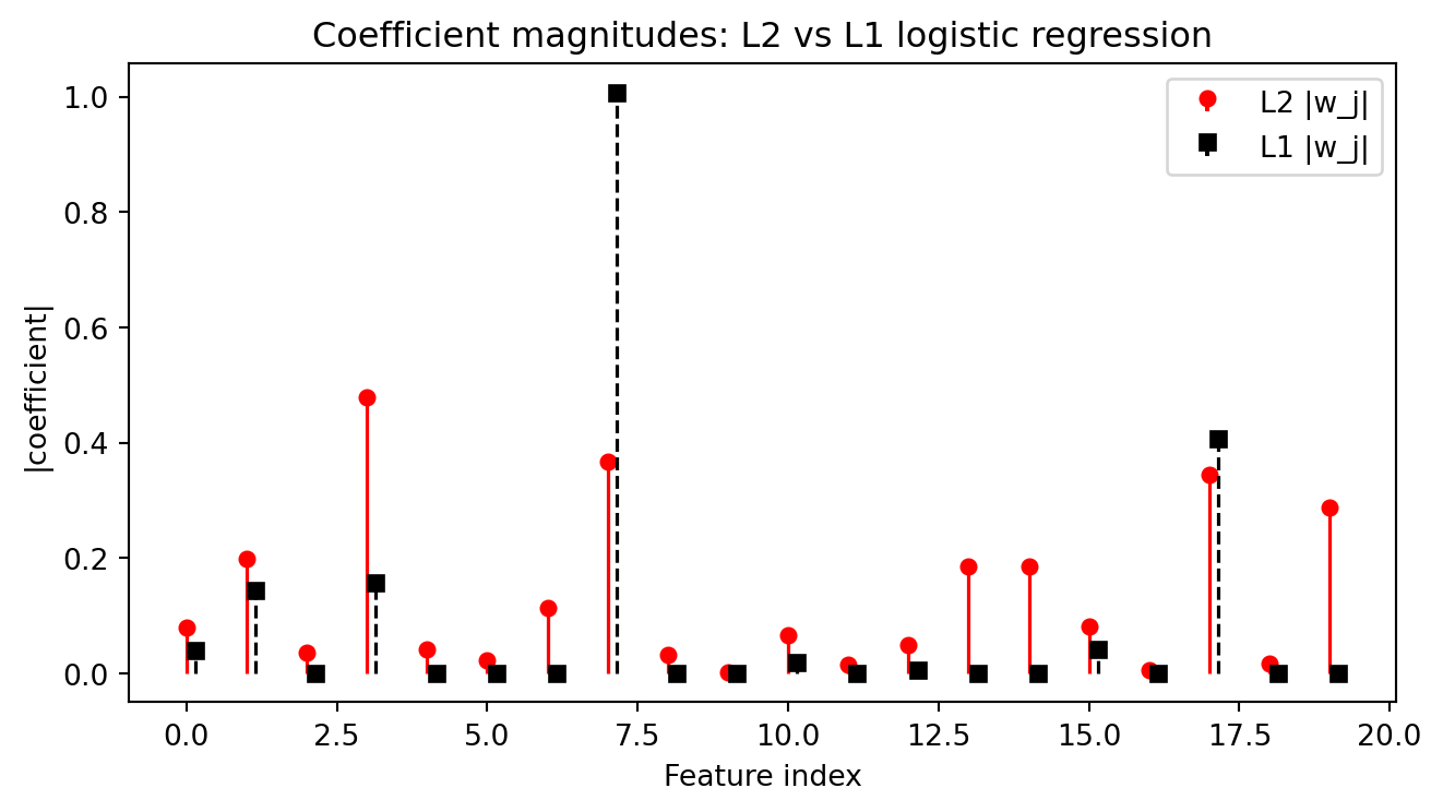
Visualizing coefficient patterns

Code
indices = np.arange(len(l2_coef))

plt.figure(figsize=(7, 4))

# Absolute values so we only care about magnitude, not sign
markerline1, stemlines1, baseline1 = plt.stem(
    indices,
    np.abs(l2_coef),
    basefmt=" ",
    label="L2 |w_j|",
)

markerline2, stemlines2, baseline2 = plt.stem(
    indices + 0.15,
    np.abs(l1_coef),
    basefmt=" ",
    label="L1 |w_j|",
)

# Format L2: circles, solid stems
plt.setp(markerline1, marker='o', markersize=5, color='red')
plt.setp(stemlines1, linewidth=1.2, color='red')

# Format L1: squares, dashed stems
plt.setp(markerline2, marker='s', markersize=5, color='black')
plt.setp(stemlines2, linewidth=1.2, linestyle='--', color='black')

plt.xlabel("Feature index")
plt.ylabel("|coefficient|")
plt.title("Coefficient magnitudes: L2 vs L1 logistic regression")
plt.legend()
plt.tight_layout()
plt.show()

What to notice

  • For L2:
    • Many features get small, but non-zero, coefficients.
    • Noise features still carry a bit of weight (“soft” shrinkage).
  • For L1:
    • Many coefficients are exactly zero.
    • A small subset of features carry most of the weight.
    • This is the classic sparsity / feature selection effect of L1.

✏️ Try:

  • Changing C_value (smaller = stronger regularization).
  • Increasing n_features or n_informative in make_classification.
  • Seeing how the balance between accuracy and sparsity changes.

Choosing \(\lambda\): tuning regularization strength

We usually do not set \(\lambda\) by hand.

Instead:

  1. Choose a grid of candidate values (e.g., \(\lambda \in \{10^{-3}, 10^{-2}, \dots, 10^{2}\}\)).
  2. For each \(\lambda\):
    • Train the model.
    • Estimate performance via cross-validation (from M13).
  3. Pick the \(\lambda\) that gives the best validation performance (or best tradeoff).

Low \(\lambda\)

  • Weak regularization.
  • Fit focuses heavily on training loss.
  • Risk of overfitting.

High \(\lambda\)

  • Strong regularization.
  • Model parameters heavily shrunk.
  • Risk of underfitting.

Ethics & risks

Even though regularization is a mathematical tool, its use has ethical implications:

  • Fairness:
    • Regularization can hide systematic bias rather than address it.
    • Example: a sparse model may still rely on a single proxy feature for a protected attribute.
  • Interpretability vs. misuse:
    • L1 can make models easier to explain.
    • But “sparse ≠ fair” and “sparse ≠ causal”.
  • Robustness:
    • Regularization often improves robustness to random noise.
    • But it does not automatically protect against adversarial inputs or distribution shift.

Curiosity: connections to deep learning

Regularization ideas show up everywhere in deep learning:

  • Weight decay:
    • Standard L2 regularization in neural network training.
  • Dropout:
    • Randomly zeroing activations during training acts as a form of regularization.
    • You’ll see this more in a future module.
  • Batch normalization & data augmentation:
    • Help stabilize training and improve generalization; often considered “implicit” regularizers.
  • Transformers & large language models:
    • Strong regularization and careful tuning are critical to prevent overfitting huge models to static datasets.

Quick checks

Q1 — Conceptual: Which of the following best describes the main purpose of regularization?

A. To reduce training error as much as possible.
B. To reduce model capacity and improve generalization.
C. To make optimization faster regardless of generalization.
D. To ensure weights are exactly zero.

Q2 — L1 vs L2: Compared to L2 regularization, L1 regularization is more likely to:

A. Increase the number of nonzero weights.
B. Decrease the number of nonzero weights.
C. Leave the number of nonzero weights unchanged.
D. Have no effect on the sparsity of the model.

Q3 — Tuning \(\lambda\): You increase \(\lambda\) for an L2-regularized model and observe:

  • Training loss increases slightly.
  • Validation loss decreases significantly.

Which is the most reasonable conclusion?

A. You should probably keep the larger \(\lambda\).
B. You should reduce \(\lambda\) back to its original value.
C. Regularization is not needed.
D. The model is definitely underfitting now.

Q4 — Short numeric reasoning: Suppose you fit two models on the same data:

  • Model A: training MSE = 0.1, validation MSE = 0.5
  • Model B (with L2): training MSE = 0.2, validation MSE = 0.3

Which model would you prefer for deployment and why (short answer)?

Further resources (optional)

Textbook chapters

  • Hastie, Tibshirani, and Friedman (2009): The Elements of Statistical Learning: Data Mining, Inference, and Prediction (2nd ed.).
    🔗Free PDF

  • Shalev-Shwartz and Ben-David (2014): Understanding Machine Learning: From Theory to Algorithms.
    🔗Free PDF

Shorter notes & classic papers

References

Hastie, Trevor, Robert Tibshirani, and Jerome Friedman. 2009. The Elements of Statistical Learning: Data Mining, Inference, and Prediction. 2nd ed. New York, NY: Springer.
Shalev-Shwartz, Shai, and Shai Ben-David. 2014. Understanding Machine Learning: From Theory to Algorithms. Cambridge, UK: Cambridge University Press.
Tibshirani, Robert. 1996. “Regression Shrinkage and Selection via the Lasso.” Journal of the Royal Statistical Society: Series B (Methodological) 58 (1): 267–88.
