M08: Maximum likelihood estimation — principle & examples

CSCI 3151: Foundations of Machine Learning

Frank Rudzicz

Where we are in the course

• Cluster C03 — MLE & EM, module M08.
• Previous modules:
  • M04–M05: supervised regression and classification as risk minimization.
• Next modules:
  • M09–M10: latent variables and EM build directly on today’s MLE idea.

• Now: focus on
  • turning data into parameter estimates \(\hat\theta\);
  • reading and plotting likelihoods;
  • connecting likelihood to decision‑aligned metrics.

Outcomes

By the end of this module you should be able to:

1. Define likelihood and maximum likelihood estimation (MLE) in precise language.
2. Recognize (if not write down) the likelihood and log‑likelihood for simple models (Bernoulli, Gaussian).
3. Compute and visualize MLEs from data using Python (pandas, numpy, matplotlib).
4. Compare models using held‑out log‑likelihood / cross‑entropy, tied to a decision context.
5. Name at least two threats to valid likelihood‑based inference (e.g., leakage, model mismatch).

Role play:
Choosing a campaign subject line

Imagine you work for a non‑profit running an email donation campaign.

• You test a new subject line
  “Match your gift today!”.
• For each email:
  • \(x\) = features of the recipient
    (we will ignore them today),
  • \(y \in \{0,1\}\) = clicked the donation link within 48 hours.
• You send the email to \(n\) people and record clicks.

• Decision: Ship the new subject line to everyone or keep the old one?

• Costs of errors:

  • Saying “it’s better” when it’s not → wasted effort, donor fatigue.
  • Missing a real improvement → fewer donations for the cause.

🧠 We will:

1. Treat each email as a Bernoulli trial with parameter \(p = P(\text{click})\).
2. Use maximum likelihood to estimate \(p\).
3. Use held‑out log‑likelihood / cross‑entropy to compare subject lines.

🛠️ DGP → model → likelihood

• Data‑generating process (DGP): The (usually unknown) story that produces
  data in the world.
  • e.g. “Each recipient independently clicks with probability \(p\).”
• Model \(p_\theta(x)\): A simplified mathematical family we choose to approximate the DGP.
  • e.g. Bernoulli(\(p\)) with parameter \(\theta = p\).
• Parameters \(\theta\): Numbers that specify a particular model in the family.
  • e.g. \(p = 0.1\) vs \(p = 0.25\).

Likelihood \(L(\theta; \mathcal{D})\)

• Treat data as fixed: \(\mathcal{D} = \{x_1,\dots,x_n\}\).
• Treat parameters as variable: \(\theta\) can move.
• Likelihood is:
  \[L(\theta; \mathcal{D}) = p_\theta(\mathcal{D})\] seen as a function of \(\theta\).

We use likelihood to score how compatible each \(\theta\) is with the observed data.

Why log‑likelihood?

Why do we often work with log‑likelihood \(\log L(\theta)\) instead of raw likelihood \(L(\theta)\)?

• Same maximizer.
  • \(\color{blue}{\log}\) is strictly increasing, so
    \[\arg\max_\theta L(\theta; \mathcal{D}) = \arg\max_\theta \color{blue}{\log} L(\theta; \mathcal{D}).\]
• Products → sums.
  • For IID data \(L(\theta; \mathcal{D}) = \prod_i p_\theta(x_i)\),
    \[\log L(\theta; \mathcal{D}) = \sum_i \log p_\theta(x_i).\]
  • Easier to differentiate, reason about, and implement.

• Numerical stability.
  • Raw likelihoods can be extremely small; logs keep values in a range amenable to computation.
• Direct link to loss.
  • In ML we typically minimize negative log‑likelihood:
    \[\mathcal{L}(\theta) = -\log L(\theta; \mathcal{D}),\] which is exactly the training loss for many models (e.g., cross‑entropy for classification).

❌ Abusing likelihood

Suppose we:

1. Train a classifier on all labeled data (no train/test split).
2. Compute the likelihood / accuracy on that same data.
3. Declare: “Our model is extremely likely / accurate, so we are done.” 🎉

Problems:

• ❌ Data leakage: we never evaluated on unseen data, so the likelihood does not test generalization.
• ❌ Wrong direction of inference: high \(p_\theta(\mathcal{D})\) does not mean high \(p(\theta \mid \mathcal{D})\) without extra assumptions. The model isn’t likely – the data are.
• ❌ Model mismatch: a mis‑specified model can still be sharp and wrong.

Take‑away

Likelihood is a useful scoring rule, not a guarantee of truth. We still need splits, baselines, and robustness checks.

🔬 Definition of MLE

Let \(\mathcal{D} = \{x_1,\dots,x_n\}\) be IID samples from some model \(p_\theta(x)\).

• Likelihood:
  \[L(\theta; \mathcal{D}) = \prod_{i=1}^n p_\theta(x_i).\]

• Log‑likelihood:
  \[\log L(\theta; \mathcal{D}) = \sum_{i=1}^n \log p_\theta(x_i).\]

• Maximum likelihood estimator (MLE): \[\hat\theta_{\text{MLE}} = \mathop{\mathrm{arg\,max}}_\theta \log L(\theta; \mathcal{D}).\]

🧠 Key idea

If you ever find some other parameter \(\theta'\) with
\(\log L(\theta'; \mathcal D) > \log L(\hat{\theta}; \mathcal D)\),
in a sense \(\theta'\) would be more insistent on \(\mathcal D\) being true, making it a better representation of the data.

We’ll now look at two concrete examples.

Example 1: Bernoulli clicks

• 🛢️ Data: \(y_i \in \{0,1\}\), \(i=1,\dots,n\), IID
• 🧮 Model: \(Y_i \sim \text{Bernoulli}(p)\) with parameter \(\theta = p\).
• Likelihood: \[ L(p; \mathcal{D}) = \prod_{i=1}^n p^{y_i} (1-p)^{1-y_i} = p^{\sum y_i} (1-p)^{n - \sum y_i}. \]
• Let \(k = \sum_{i=1}^n y_i\) be the number of clicks. \[ \log L(p; \mathcal{D}) = k \log p + (n-k)\log(1-p). \]
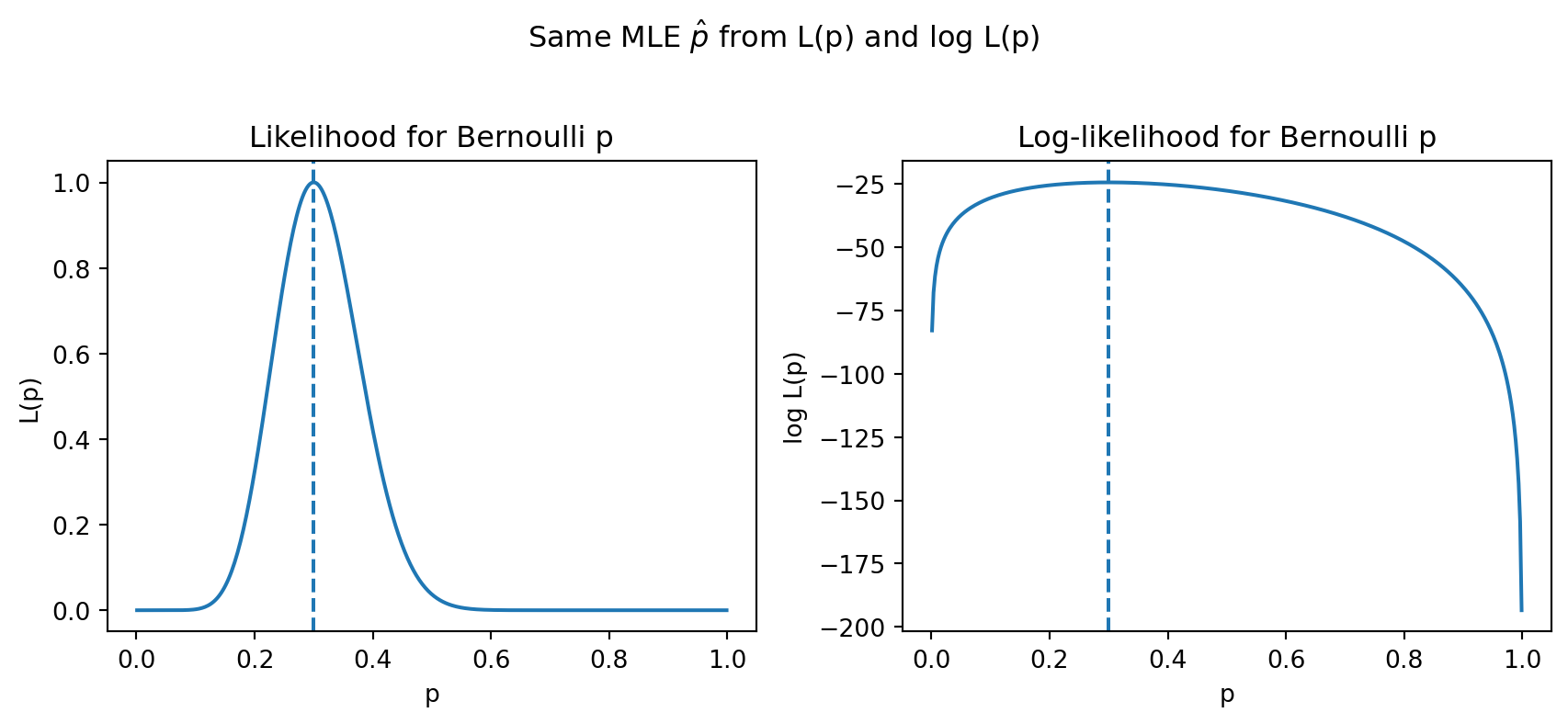
• Take derivative and set to zero: \[ \frac{d\log L}{dp} = \frac{k}{p} - \frac{n-k}{1-p} = 0 \quad\Rightarrow\quad \hat p_{\text{MLE}} = \frac{k}{n}. \]

Likelihood vs log-likelihood
(same optimum)

import numpy as np
import matplotlib.pyplot as plt

# Example: k successes out of n trials

n = 40
k = 12

p_grid = np.linspace(0.001, 0.999, 400)

# Log-likelihood (up to an additive constant)

log_L = k * np.log(p_grid) + (n - k) * np.log(1 - p_grid)

# Rescaled likelihood to avoid overflow and keep it on a nice scale

L = np.exp(log_L - log_L.max())

p_hat = k / n

fig, axes = plt.subplots(1, 2, figsize=(9, 4))

# Left: likelihood

ax = axes[0]
ax.plot(p_grid, L)
ax.axvline(p_hat, linestyle="--")
ax.set_xlabel("p")
ax.set_ylabel("L(p)")
ax.set_title("Likelihood for Bernoulli p")

# Right: log-likelihood

ax = axes[1]
ax.plot(p_grid, log_L)
ax.axvline(p_hat, linestyle="--")
ax.set_xlabel("p")
ax.set_ylabel("log L(p)")
ax.set_title("Log-likelihood for Bernoulli p")

fig.suptitle("Same MLE $\hat p$ from L(p) and log L(p)", y=1.02)
fig.tight_layout()
plt.show()

Example 2: Gaussian heights

🛢️ Data: \(x_i \in \mathbb{R}\) (e.g., measured heights in cm).
🧮 Model: \(X_i \sim \mathcal{N}(\mu, \sigma^2)\) IID.

Likelihood:

\[ L(\mu,\sigma^2; \mathcal{D}) = \prod_{i=1}^n \frac{1}{\sqrt{2\pi\sigma^2}} \exp\!\left( -\frac{(x_i-\mu)^2}{2\sigma^2} \right). \]

Log‑likelihood (ignoring constants):

\[ \log L(\mu,\sigma^2) = -\frac{n}{2}\log\sigma^2 -\frac{1}{2\sigma^2}\sum_{i=1}^n (x_i-\mu)^2 + C. \]

Optimizing:

• \(\hat\mu_{\text{MLE}} = \frac{1}{n}\sum_i x_i\) (the sample mean),

• \(\hat\sigma^2_{\text{MLE}} = \frac{1}{n} \sum_i (x_i-\hat\mu)^2\).

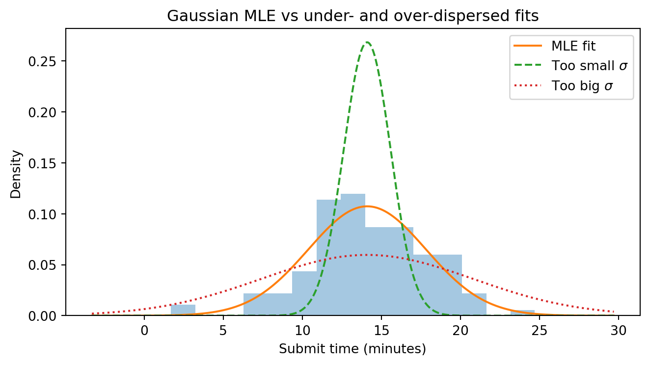
👉 The MLE for \(\sigma^2\) uses \(1/n\) (not \(1/(n-1)\)). The latter is the ‘unbiased estimator’.

Gaussian MLE vs
under- / over-dispersed fits

import numpy as np
import matplotlib.pyplot as plt
from scipy.stats import norm  # if you prefer, you can hand-code the pdf

np.random.seed(3151)

# Synthetic "time to submit quiz" data (in minutes)

mu_true = 15.0
sigma_true = 4.0
n = 120
times = np.random.normal(mu_true, sigma_true, size=n)

# MLEs for mu and sigma^2

mu_hat = np.mean(times)
sigma_hat = np.std(times, ddof=0)

# A couple of deliberately "bad" sigmas for illustration

sigma_too_small = sigma_hat * 0.4
sigma_too_big = sigma_hat * 1.8

x_grid = np.linspace(times.min() - 5, times.max() + 5, 400)

fig, ax = plt.subplots(figsize=(7, 4))

# Histogram of data

ax.hist(times, bins=15, density=True, alpha=0.4)

# MLE fit

ax.plot(x_grid, norm.pdf(x_grid, loc=mu_hat, scale=sigma_hat),
label="MLE fit")

# Too narrow

ax.plot(x_grid, norm.pdf(x_grid, loc=mu_hat, scale=sigma_too_small),
linestyle="--", label="Too small $\sigma$")

# Too wide

ax.plot(x_grid, norm.pdf(x_grid, loc=mu_hat, scale=sigma_too_big),
linestyle=":", label="Too big $\sigma$")

ax.set_xlabel("Submit time (minutes)")
ax.set_ylabel("Density")
ax.set_title("Gaussian MLE vs under- and over-dispersed fits")
ax.legend()
fig.tight_layout()
plt.show()

Example 3: Poisson counts 🐟

🛢️ Data: \(k_i \in \{0,1,2,\dots\}\) = number of events in a fixed time window (e.g., password reset requests per hour).
🧮 Model: \(K_i \sim \text{Poisson}(\lambda)\) IID.

Likelihood:

\[ L(\lambda; \mathcal{D}) = \prod_{i=1}^n \frac{e^{-\lambda}\lambda^{k_i}}{k_i!}. \]

Log‑likelihood (dropping constants that do not depend on \(\lambda\)):

\[ \begin{align} \log L(\lambda) &= \sum_{i=1}^n \big(k_i \log\lambda - \lambda\big)\\ &= \left(\sum_{i=1}^n k_i\right)\log\lambda - n\lambda + C. \end{align} \]

Differentiate and set to zero:

\[ \begin{align} \frac{\partial \log L}{\partial \lambda} &= \frac{\sum_i k_i}{\lambda} - n = 0 \quad\Rightarrow\\ \quad\hat\lambda_{\text{MLE}} &= \frac{1}{n}\sum_{i=1}^n k_i. \end{align} \]

Again the MLE is a familiar empirical statistic: the sample mean count.

Examples

E.g. 1: MLE for click‑through rate

Tiny synthetic dataset inspired by the email campaign:

• Each row = one email sent (unit: email impression).
• clicked = 1 if the recipient clicked within 48 hours, else 0.

import numpy as np
import pandas as pd
import matplotlib.pyplot as plt

rng = np.random.default_rng(3151)

n = 40                       # number of emails
true_p = 0.30                # true (hidden) click probability

clicks = rng.binomial(1, true_p, size=n)
df = pd.DataFrame({"clicked": clicks})

# Small summary table
summary = (
    df["clicked"]
      .value_counts()
      .rename(index={0: "no_click", 1: "click"})
      .rename("count")
      .reset_index()
      .rename(columns={"index": "outcome"})
)
summary

	outcome	count
0	no_click	28
1	click	12

k = df["clicked"].sum()
n = len(df)
p_mle = k / n

print(f"Number of clicks k = {k} out of n = {n}")
print(f"Empirical click‑through rate (MLE) p_hat = {p_mle:.3f}")

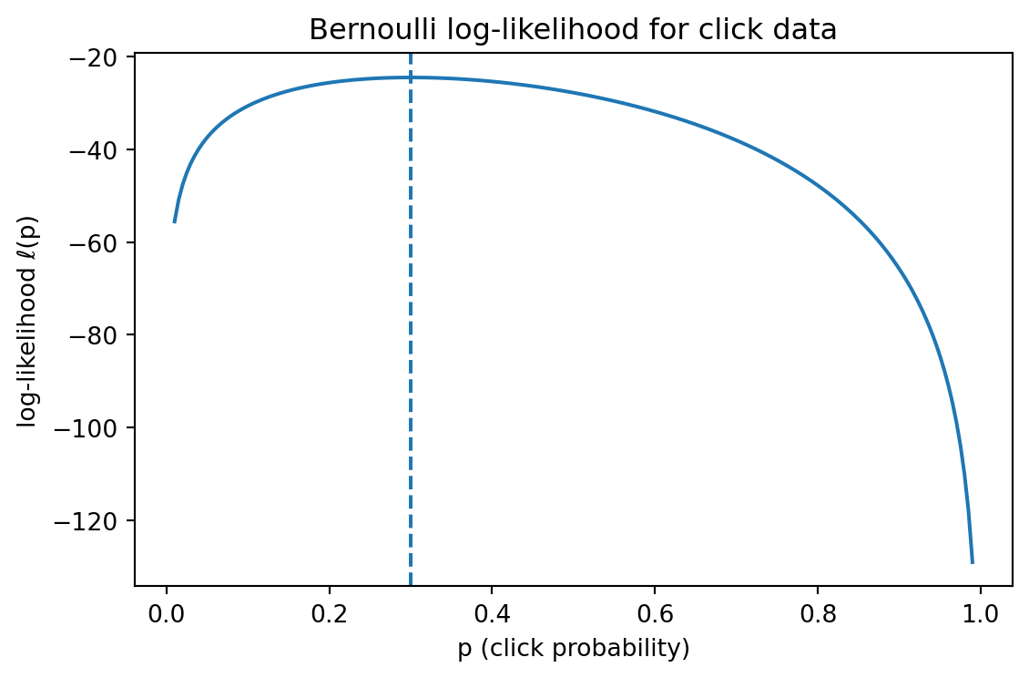
p_vals = np.linspace(0.01, 0.99, 200)
log_like = k * np.log(p_vals) + (n - k) * np.log(1 - p_vals)

plt.figure(figsize=(6, 4))
plt.plot(p_vals, log_like)
plt.axvline(p_mle, linestyle="--")
plt.xlabel("p (click probability)")
plt.ylabel("log-likelihood ℓ(p)")
plt.title("Bernoulli log-likelihood for click data")
plt.tight_layout()
plt.show()

Number of clicks k = 12 out of n = 40
Empirical click‑through rate (MLE) p_hat = 0.300

Observe: the log‑likelihood is maximized exactly at the empirical click rate.

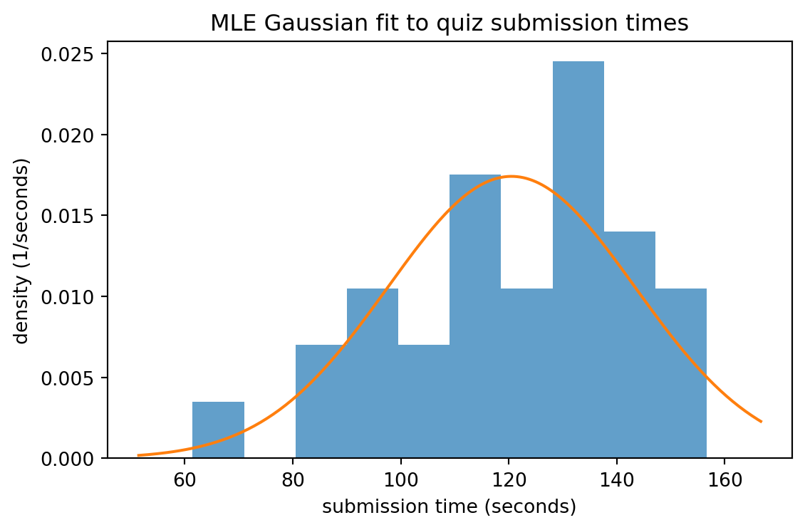
E.g. 2: MLE for Gaussian \(\mu\) and \(\sigma\)

Now imagine we measured the time (in seconds) it took students to submit an online quiz after it opens.

• Each row = one student’s submission time.
• We model times as approximately Gaussian (after a log / standardization step in real life).

import numpy as np
import pandas as pd
import matplotlib.pyplot as plt

rng = np.random.default_rng(42)
n = 30
true_mu = 120.0   # seconds
true_sigma = 30.0 # seconds

times = rng.normal(loc=true_mu, scale=true_sigma, size=n)
df_times = pd.DataFrame({"submit_time_sec": times})

df_times.head()

	submit_time_sec
0	129.141512
1	88.800477
2	142.513536
3	148.216941
4	61.468944

mu_mle = df_times["submit_time_sec"].mean()
sigma2_mle = ((df_times["submit_time_sec"] - mu_mle) ** 2).mean()
sigma_mle = np.sqrt(sigma2_mle)

summary_params = pd.DataFrame(
    {
        "parameter": ["mu_hat", "sigma_hat"],
        "estimate": [mu_mle, sigma_mle],
        "units": ["seconds", "seconds"]
    }
)
summary_params

	parameter	estimate	units
0	mu_hat	120.504424	seconds
1	sigma_hat	22.910806	seconds

plt.figure(figsize=(6, 4))
plt.hist(df_times["submit_time_sec"], bins=10, density=True, alpha=0.7)

x = np.linspace(
    df_times["submit_time_sec"].min() - 10,
    df_times["submit_time_sec"].max() + 10,
    200
)

def normal_pdf(x, mu, sigma):
    return (1.0 / (np.sqrt(2 * np.pi) * sigma)) * np.exp(-(x - mu)**2 / (2 * sigma**2))

plt.plot(x, normal_pdf(x, mu_mle, sigma_mle))
plt.xlabel("submission time (seconds)")
plt.ylabel("density (1/seconds)")
plt.title("MLE Gaussian fit to quiz submission times")
plt.tight_layout()
plt.show()

Again, the MLE picks parameters that best explain the observed histogram under the Gaussian model.

Numerical MLE demo:
Logistic regression in 1D

So far our examples had closed‑form MLEs.
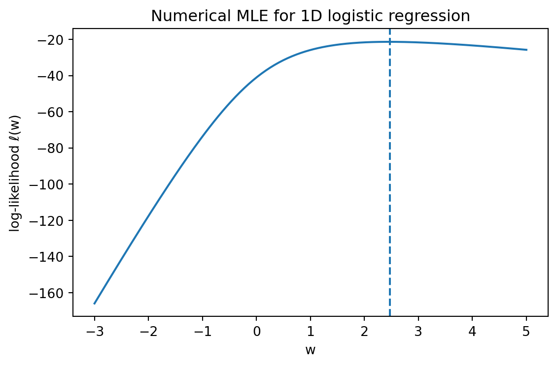
For many ML models (e.g., logistic regression, neural nets) there is no algebraic solution — we find \(\hat\theta\) numerically/approximately.

Consider a tiny 1D logistic regression:

• Feature \(x\) = a relevance score for each email.
• Label \(y \in \{0,1\}\) = clicked or not.
• Model: \(p_\theta(y=1\mid x) = \sigma(w x + b)\), where \(\sigma(z) = \frac{1}{1+e^{-z}}\).
• Parameters \(\theta = (w,b)\).

Even if we fix \(b\), there is no closed form for the MLE of \(w\).

import numpy as np
import matplotlib.pyplot as plt

rng = np.random.default_rng(8)

n = 60
x = rng.normal(size=n)
w_true, b_true = 2.0, -0.3
p_true = 1 / (1 + np.exp(-(w_true * x + b_true)))
y = rng.binomial(1, p_true)

def log_likelihood(w):
    z = w * x + b_true
    p = 1 / (1 + np.exp(-z))
    # clip to avoid log(0)
    eps = 1e-9
    p = np.clip(p, eps, 1 - eps)
    return np.sum(y * np.log(p) + (1 - y) * np.log(1 - p))

w_grid = np.linspace(-3, 5, 200)
ll_vals = np.array([log_likelihood(w) for w in w_grid])
w_hat = w_grid[ll_vals.argmax()]

plt.figure(figsize=(6, 4))
plt.plot(w_grid, ll_vals)
plt.axvline(w_hat, linestyle="--")
plt.xlabel("w")
plt.ylabel("log-likelihood ℓ(w)")
plt.title("Numerical MLE for 1D logistic regression")
plt.tight_layout()
plt.show()

Here we find \(\hat w\) by a simple grid search over candidate values.

• In real models we use gradient‑based optimization (e.g., gradient ascent, stochastic gradient descent, Newton’s method).
• Key idea: MLE becomes a generic numerical optimization problem once we can compute the log‑likelihood and its gradient.

Evaluation aligned to decisions

In practice, we rarely look at raw likelihoods. Instead we use:

• Average negative log‑likelihood (NLL) on a held‑out set:
  \[\text{NLL} = -\frac{1}{n_\text{val}} \sum_{i=1}^{n_\text{val}} \log p_{\hat\theta}(x_i^{\text{(val)}}).\]
• For binary classification this is exactly cross‑entropy loss.

Decision‑alignment:

• Over‑confident wrong predictions get large penalties → good when bad decisions are costly.
• Comparing two models by held‑out NLL answers:
  > “Which model assigns higher probability to what actually happened?”

Always:

1. Keep a clean validation / test split (no peeking when fitting).
2. Compare against simple baselines (e.g., always predict average click rate).

Ethics nudge: risks & mitigations

• Biased data → biased likelihoods.
  If historical data under‑represent certain groups, MLE will faithfully reproduce those biases.
  • Mitigate by checking performance / likelihood by subgroup and considering fairness constraints.
• Privacy and re‑identification.
  Likelihood models over detailed user logs can leak information (e.g., via membership inference attacks).
  • Mitigate with data minimization, aggregation, and privacy‑preserving training (e.g., DP, secure aggregation) where appropriate.

Quick check (pause video here!)

1. MCQ. In maximum likelihood, which of the following is treated as a function argument?

   • 1. The data \(\mathcal{D}\)
        
   • 2. The parameters \(\theta\)
        
   • 3. The model class (e.g. “all Gaussians”)
        
   • 4. The learning rate

2. Numeric. We flip a coin \(n = 10\) times and observe \(k = 7\) heads. What is the MLE \(\hat p\) for the probability of heads?

3. MCQ. Which statement about log‑likelihood is correct?

   • 1. Taking logs changes which parameter maximizes likelihood.
        
   • 2. Log‑likelihood is always negative, so it cannot be used for model comparison.
        
   • 3. Maximizing log‑likelihood is equivalent to maximizing likelihood.
        
   • 4. Log‑likelihood does not depend on the data.

4. Short answer. Name one threat to using MLE in a real ML system and how you would detect it.

Properties of MLE (in one breath)

Under mild regularity conditions (IID data, well‑behaved model family), MLEs have powerful theoretical guarantees:

• Consistency. As \(n \to \infty\), \(\hat\theta_{\text{MLE}}\) converges in probability to the true parameter \(\theta^\star\) (if the model is correctly specified).
• Asymptotic normality. For large \(n\), \[\hat\theta_{\text{MLE}} \approx \mathcal{N}\!\big(\theta^\star,\; I(\theta^\star)^{-1}/n\big),\] where \(I(\theta^\star)\) is the Fisher information.
• Efficiency (asymptotic). Among a broad class of reasonable estimators, MLE attains the smallest possible variance in large samples.
• Invariance. If \(\hat\theta\) is the MLE of \(\theta\) and \(\phi = g(\theta)\) is a one‑to‑one reparameterization, then \(g(\hat\theta)\) is the MLE of \(\phi\).

We won’t prove these results in this module, but they explain why MLE is a default choice in many statistics and ML pipelines.

Summary

• Likelihood scores how compatible a parameter choice is with observed data.
• MLE chooses parameters that maximize log‑likelihood, often matching familiar empirical statistics:
  • Bernoulli: mean of 0/1 outcomes,
  • Gaussian: sample mean and variance (with \(1/n\)).
• In practice we evaluate models via held‑out NLL / cross‑entropy, respecting the ML pipeline:
  • clean splits, baselines, and clear decision contexts.
• MLE is powerful but fragile if the DGP, model, or data pipeline are wrong → always look for severe tests and replication.