M05: From regression to logistic regression

CSCI 3151: Foundations of Machine Learning

Frank Rudzicz

2025-11-23

Assumptions

By M05, we assume:

• You’ve watched M04 and are comfortable with:
  • Linear regression in 1D and \(n\)-D.
  • Squared loss for a single example and the empirical risk (average loss).
  • The basic supervised learning pipeline and the idea of train/test splits.
• You are comfortable with:
  • NumPy, pandas, matplotlib, and basic scikit-learn regression APIs.

We do not assume you’ve seen logistic regression derivations before.

Outcomes

By the end of this module, you should be able to:

• Explain why naive linear regression is a poor model for binary classification.
• Define the logistic regression model: linear score + sigmoid → probability.
• Write down the logistic (cross-entropy) loss and connect it to empirical risk.
• Derive (or follow) the gradient of the logistic loss for a single example (stretch).
• Implement and evaluate logistic regression in Python on a small dataset.
• Compare logistic regression to a naive regression-based classifier and a constant baseline.
• Apply basic train/test and leakage heuristics in a classification setting.

Recap: supervised regression

From M04:

• We model a real-valued target \(t \in \mathbb{R}\) as \[ y = f_\theta(x) = w_1^\top x + w_0. \]
• We use squared loss per example: \[ \ell( y, t ) = \frac{1}{2} (y - t)^2. \]
• For a dataset \(\{(x^{(i)}, t^{(i)})\}_{i=1}^n\), we minimize empirical risk: \[ \hat{L}_n(\theta) = \frac{1}{n}\sum_{i=1}^n \ell\big(f_\theta(x^{(i)}), t^{(i)}\big). \]

☺️ This works well when:

• The noise looks roughly Gaussian.
• The target is real-valued with a meaningful scale.
• We don’t need probabilities, just point predictions.

New goal: binary classification

Now \(y \in \{0,1\}\), e.g.,

• \(y=1\): engine has a failure within 24 flight hours.
• \(y=0\): engine remains normal.

We want:

• \(\hat{p}(y=1\mid x)\) in [0,1], interpretable as a probability.
• A model trained by minimizing an appropriate classification loss.
• A decision rule (threshold) that matches our costs.

Example: jet-engine early warning

Imagine an airline monitoring jet engines. For each engine, we log telemetry from the first few minutes of a flight:

• Features (simplified):
  • vibration_rms (RMS vibration, in g)
  • oil_temp_delta (oil temperature above nominal, in °C)
• 🎯 Target:
  • \(y \in \{0,1\}\) where
    1 = failure within the next 24 flight hours,
    0 = normal operation.

🤔 Decision:

Flag engines that are likely to fail soon so maintenance can intervene.

👀 We’d like:

• Predictions \(\hat{p}(y=1\mid x)\) in [0,1] we can interpret as probabilities.
• To trade off false negatives (missed at-risk engines) vs false positives (extra inspections).

Naïvely lin regresssing

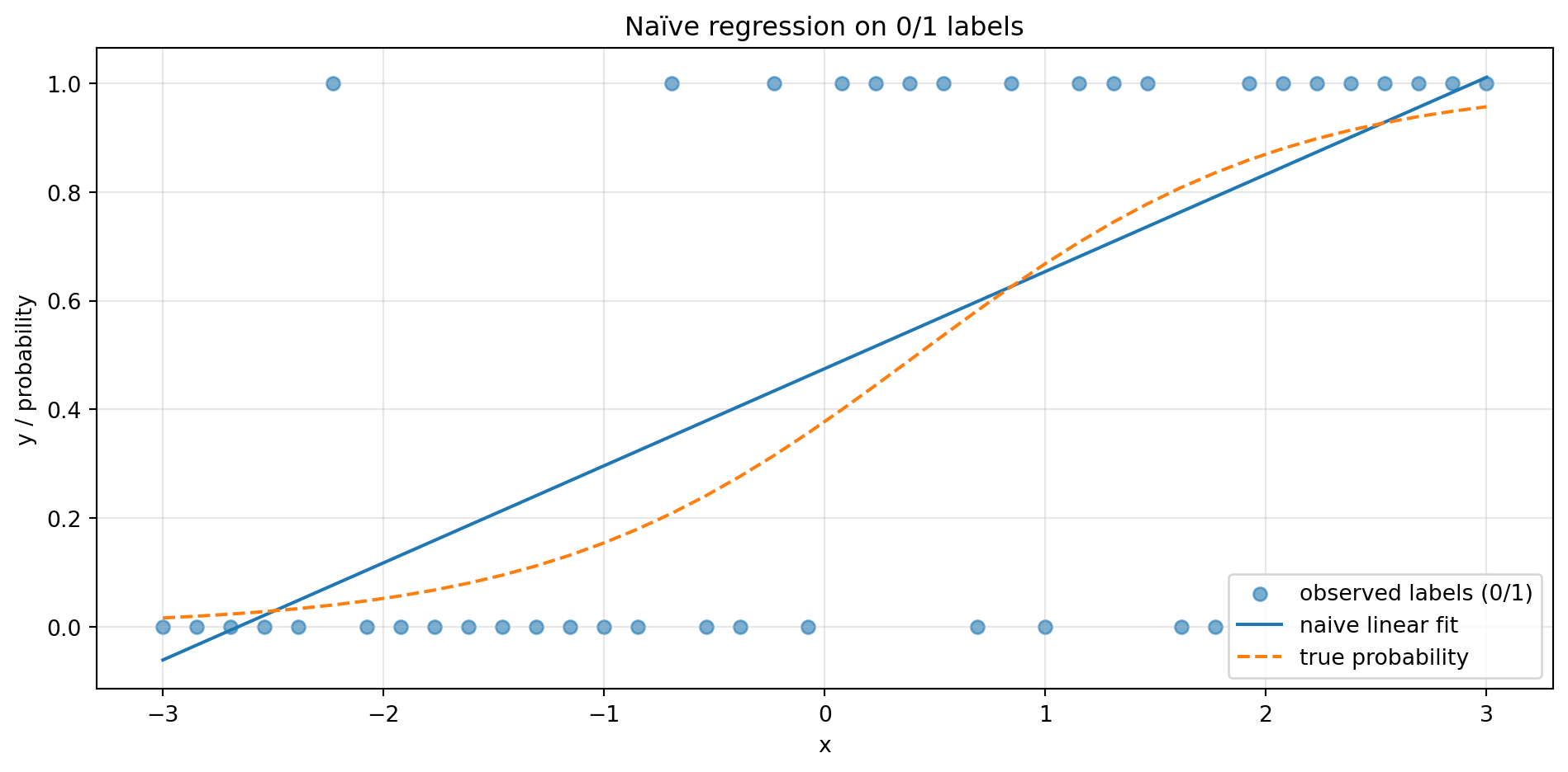
Try to treat \(y\in\{0,1\}\) as a continuous target and use linear regression:

1. Fit \[ \hat{y} = w_1^\top x + w_0 \] by minimizing squared loss.

2. Interpret \(\hat{y}\) as a “probability” and clip to [0,1] if needed.

3. Threshold at 0.5 to predict class 1 vs 0.

Problems:

• No guarantee that \(\hat{y}\) lies in [0,1].
• Squared loss does not reflect probabilistic correctness.
• 🧑‍🏫 Over-confident wrong predictions are not penalized as harshly as they should.

Small synthetic 1D example

Figure 1: Naïve linear regression fit on 0/1 labels.

👀 Notice:

• The linear fit can go below 0 or above 1.
• The relationship between \(x\) and the probability of \(y=1\) is clearly non-linear.
• We want a model that respects the [0,1] range and the probabilistic structure.

Sigmoid shape

z = np.linspace(-8, 8, 400)
sigma = 1 / (1 + np.exp(-z))

fig, ax = plt.subplots()
ax.plot(z, sigma)
ax.set_xlabel("z")
ax.set_ylabel("sigma(z)")
ax.set_title("Sigmoid function")
ax.axhline(0.5, color="gray", linestyle="--")
ax.axvline(0, color="gray", linestyle="--")
plt.tight_layout()
plt.show()

Figure 2: Sigmoid function mapping real-valued scores to probabilities.

• For very negative \(z\), \(\sigma(z) \approx 0\) (confident “class 0”).
  
• For very positive \(z\), \(\sigma(z) \approx 1\) (confident “class 1”).
  
• Around \(z=0\), the function is steep: small changes in \(z\) significantly change the probability.

Logistic regression: idea

Logistic regression fixes this by modelling the probability of class 1 directly.

1. Compute a linear score: \[ z = \theta^\top x = w_1^\top x + w_0. \]

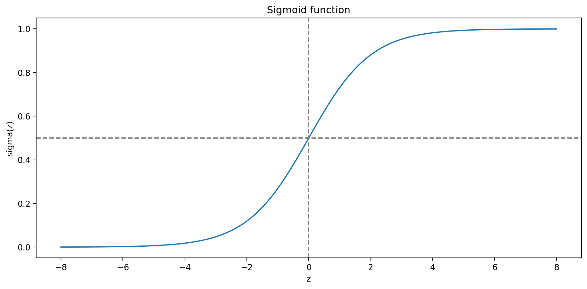
2. Squash it with the sigmoid: \[ \sigma(z) = \frac{1}{1 + e^{-z}}. \]

3. Interpret: \[ \hat{p}(y=1 \mid x) = \sigma( \theta^\top x). \]

This guarantees \(\hat{p} \in (0,1)\) and fits naturally with a Bernoulli likelihood.

Logistic (cross-entropy) loss

Let \(y \in \{0,1\}\) and \(\hat{p} = \hat{p}(y=1 \mid x)\).

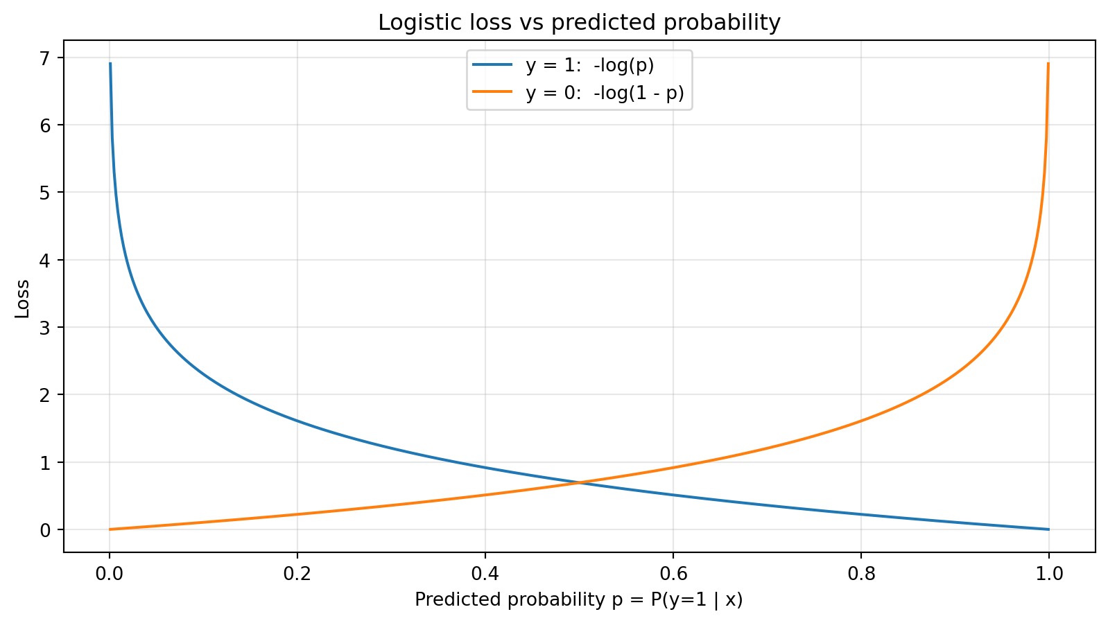
Define the logistic loss: \[ \ell_{ \text{log}}(\hat{p}, y) = -\big(y \log \hat{p} + (1-y)\log(1-\hat{p})\big). \]

Intuition:

• If \(y=1\), loss is \(-\log \hat{p}\):
  • Small if \(\hat{p}\approx 1\), large if \(\hat{p}\approx 0\).
• If \(y=0\), loss is \(-\log(1-\hat{p})\):
  • Small if \(\hat{p}\approx 0\), large if \(\hat{p}\approx 1\).

Figure 3: Logistic loss for y=1 and y=0 as a function of predicted probability p.

Logistic (cross-entropy) risk

For a dataset, empirical risk: \[ \hat{L}_n( \theta) = \frac{1}{n}\sum_{i=1}^n \ell_{\text{log}}\big(\hat{p}^{(i)}, y^{(i)}\big). \]

Training logistic regression = minimize this average loss.

When binary accuracy hides differences

Three models make identical hard predictions but different probability predictions:

import numpy as np
from sklearn.metrics import log_loss

y_true = np.array([0, 0, 1, 1])

p_A = np.array([0.49, 0.49, 0.51, 0.51])
p_B = np.array([0.1, 0.4, 0.6, 0.9])
p_C = np.array([0.01, 0.01, 0.99, 0.99])

for name, p in [("A", p_A), ("B", p_B), ("C", p_C)]:
    y_hat = (p >= 0.5).astype(int)
    acc = np.mean(y_hat == y_true)
    loss = log_loss(y_true, p)
    print(f"Model {name}: accuracy={acc:.2f}, log-loss={loss:.3f}")

Model A: accuracy=1.00, log-loss=0.673
Model B: accuracy=1.00, log-loss=0.308
Model C: accuracy=1.00, log-loss=0.010

• All three have the same binary accuracy.
• But logistic loss strongly prefers confident and correct models.
• Over-confident mistakes (e.g., high \(\hat{p}\) when \(y=0\), or vice versa) are punished most.

This is why cross-entropy / log-loss is often a better objective when our decisions depend on the probabilities, not just on the hard labels.

🔬 Gradient of logistic loss (stretch)

Model: \[ f_\theta(x) = \sigma( \theta^\top x), \quad \sigma(z) = \frac{1}{1+e^{-z}}. \]

Loss for one example \((x,y)\): \[ \ell(\theta; x, y) = -\big(y \log \sigma( \theta^\top x) + (1-y)\log(1-\sigma( \theta^\top x))\big). \]

Key result. \[ \nabla_\theta \ell( \theta; x, y) = \big(\sigma( \theta^\top x) - y\big)\,x. \]

• Proof sketch:
  1. Let \(z = \theta^\top x\) and \(p = \sigma(z)\).
  2. Loss: \(\ell = -[y \log p + (1-y)\log(1-p)]\).
  3. Differentiate w.r.t. \(p\): \[ \frac{\partial \ell}{\partial p} = -\frac{y}{p} + \frac{1-y}{1-p} = \frac{p-y}{p(1-p)}. \]
  4. Differentiate \(p = \sigma(z)\): \[ \frac{\partial p}{\partial z} = p(1-p). \]
  5. Chain rule: \[ \frac{\partial \ell}{\partial z} = \frac{\partial \ell}{\partial p} \frac{\partial p}{\partial z} = (p-y). \]
  6. Since \(\frac{\partial z}{\partial \theta} = x\), \[\nabla_\theta \ell( \theta; x,y) = (p-y)x. \]

For a dataset, average these gradients over all examples.

🔬 Tiny numeric gradient check

import numpy as np

def logistic_loss_single(theta, x, y):
    z = theta @ x
    p = 1 / (1 + np.exp(-z))
    return -(y * np.log(p) + (1 - y) * np.log(1 - p))

def logistic_grad_single(theta, x, y):
    z = theta @ x
    p = 1 / (1 + np.exp(-z))
    return (p - y) * x

rng = np.random.default_rng(42)
theta = rng.normal(size=2)
x = rng.normal(size=2)
y = 1

eps = 1e-5
basis = np.eye(2)
num_grad = np.zeros_like(theta)

for j in range(2):
    theta_plus = theta + eps * basis[j]
    theta_minus = theta - eps * basis[j]
    num_grad[j] = (logistic_loss_single(theta_plus, x, y) -
                   logistic_loss_single(theta_minus, x, y)) / (2 * eps)

print("Analytic grad:", logistic_grad_single(theta, x, y))
print("Numeric grad: ", num_grad)

Analytic grad: [-0.50960822 -0.63870844]
Numeric grad:  [-0.50960822 -0.63870844]

🧠 Why did we do this?

• We derived a closed-form gradient using calculus, \(\nabla_\theta \ell( \theta; x,y) = (p-y)x\).
• It’s easy to make a sign or indexing mistake when you turn that into code.
• The numeric gradient check is a sanity test:
  • “If I approximate the gradient just by looking at how the loss changes when I wiggle each parameter, do I get the same answer as my analytic formula?”
• In real projects, people do this when:
  • Implementing custom losses,
  • Writing their own optimizers,
  • Or debugging backprop in neural nets.

It’s like a tiny scientific experiment: hold everything else fixed, perturb one parameter slightly, measure how the loss changes, and compare to what your math predicts should happen.

Numeric and analytic gradients should be very close (up to a small numerical error).
This is a simple way to sanity-check gradient code.

From loss to decisions

Logistic regression gives us probabilities \(\hat{p}(y=1\mid x)\).

To make a decision, we choose a threshold \(\tau\):

• Predict class 1 if \(\hat{p} \ge \tau\).
• Predict class 0 otherwise.

Choosing \(\tau=0.5\) is natural if false positives and false negatives are equally bad.

• In the early-warning scenario, missing an impending failure might be worse than sending one extra inspection, suggesting a lower threshold like \(\tau=0.3\).
  • I.e., You’d rather predict class 1 more than necessary, since false negatives are worse than false positives.

✈️ Early-warning system: data

Let’s see (the head of) some data again:

import pandas as pd
import numpy as np

rng = np.random.default_rng(3151)
n_flights = 3000

# Telemetry from the *first few minutes* of each flight (synthetic):
# - vibration_rms: RMS vibration (g)
# - oil_temp_delta: oil temperature above nominal (°C)
vibration_rms = rng.gamma(shape=2.0, scale=0.70, size=n_flights)   # mostly small, occasional spikes
oil_temp_delta = rng.normal(loc=5 + 4.0 * vibration_rms, scale=2.5, size=n_flights)
oil_temp_delta = np.clip(oil_temp_delta, 0, None)

# A steep "tipping point" risk model:
# once vibration and temperature cross a threshold together, failure risk shoots up.
risk_score = 1.3 * vibration_rms + 0.18 * oil_temp_delta
z_true = 10 * (risk_score - 3.2)
p_failure = 1 / (1 + np.exp(-z_true))
failure_24h = rng.binomial(1, p_failure)

# Real life is messy: some high-risk-looking flights are *not* failures (e.g., unusual operating conditions).
# We simulate that by flipping the label for the most extreme telemetry cases.
n_flips = int(0.10 * n_flights)
flip_idx = np.argsort(risk_score)[-n_flips:]
failure_24h[flip_idx] = 1 - failure_24h[flip_idx]

df = pd.DataFrame({
    "vibration_rms": vibration_rms,
    "oil_temp_delta": oil_temp_delta,
    "failure_24h": failure_24h,
})

df.head()

	vibration_rms	oil_temp_delta	failure_24h
0	0.640526	7.898066	0
1	1.509162	10.232553	1
2	1.981035	13.506731	1
3	1.285732	10.147697	1
4	0.942545	7.914355	0

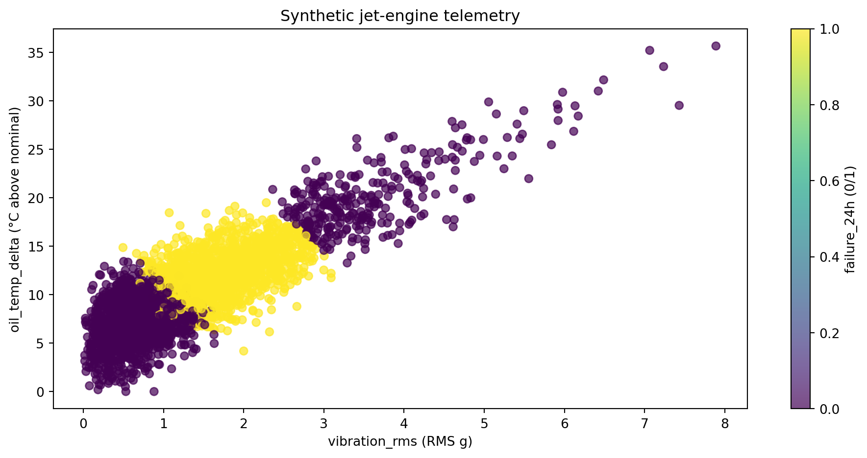
Now in scatter form (class 1: yellow; class 0: purple):

import matplotlib.pyplot as plt

fig, ax = plt.subplots()
sc = ax.scatter(df["vibration_rms"], df["oil_temp_delta"],
                c=df["failure_24h"], cmap="viridis", alpha=0.7)
ax.set_xlabel("vibration_rms (RMS g)")
ax.set_ylabel("oil_temp_delta (°C above nominal)")
ax.set_title("Synthetic jet-engine telemetry")
cbar = plt.colorbar(sc, ax=ax)
cbar.set_label("failure_24h (0/1)")
plt.tight_layout()
plt.show()

Figure 4

Train/test split &
naïve regression baseline

First, split the data into train and test with sklearn

from sklearn.model_selection import train_test_split

X = df[["vibration_rms", "oil_temp_delta"]].values
y = df["failure_24h"].values

X_train_c, X_test_c, y_train_c, y_test_c = train_test_split(
    X, y, test_size=0.25, random_state=3151, stratify=y
)

Then, train (i.e., fit) an actual LinearRegression() and get the test set accuracy

from sklearn.linear_model import LinearRegression
from sklearn.metrics import accuracy_score

lin_reg = LinearRegression()
lin_reg.fit(X_train_c, y_train_c)

train_pred_reg = lin_reg.predict(X_train_c)
test_pred_reg = lin_reg.predict(X_test_c)

# Clip to [0,1] and threshold
train_probs_reg = np.clip(train_pred_reg, 0, 1)
test_probs_reg = np.clip(test_pred_reg, 0, 1)

train_pred_labels_reg = (train_probs_reg >= 0.5).astype(int)
test_pred_labels_reg = (test_probs_reg >= 0.5).astype(int)

acc_reg = accuracy_score(y_test_c, test_pred_labels_reg)
acc_reg

0.6293333333333333

This gives us a naïve linear regression-based classifier.
We’ll compare it to logistic regression and a simple baseline.

✈️ Early-warning system:
logistic vs naïve regression

from sklearn.linear_model import LogisticRegression
from sklearn.metrics import log_loss

# Fit logistic regression
log_reg = LogisticRegression(random_state=3151)
log_reg.fit(X_train_c, y_train_c)

train_probs_lr = log_reg.predict_proba(X_train_c)[:, 1]
test_probs_lr = log_reg.predict_proba(X_test_c)[:, 1]

train_pred_labels_lr = (train_probs_lr >= 0.5).astype(int)
test_pred_labels_lr = (test_probs_lr >= 0.5).astype(int)

acc_log = accuracy_score(y_test_c, test_pred_labels_lr)

train_logloss_lr = log_loss(y_train_c, train_probs_lr)
test_logloss_lr = log_loss(y_test_c, test_probs_lr)

# Baseline: always predict training positive rate
p_base = y_train_c.mean()
train_probs_base = np.full_like(y_train_c, p_base, dtype=float)
test_probs_base = np.full_like(y_test_c, p_base, dtype=float)

train_logloss_base = log_loss(y_train_c, train_probs_base)
test_logloss_base = log_loss(y_test_c, test_probs_base)
acc_base = accuracy_score(y_test_c, (test_probs_base >= 0.5).astype(int))

import pandas as pd
results = pd.DataFrame([
    {
        "model": "baseline",
        "train_logloss": train_logloss_base,
        "test_logloss": test_logloss_base,
        "test_accuracy": acc_base
    },
    {
        "model": "naive_linear_regression",
        "train_logloss": np.nan,
        "test_logloss": np.nan,
        "test_accuracy": acc_reg
    },
    {
        "model": "logistic_regression",
        "train_logloss": train_logloss_lr,
        "test_logloss": test_logloss_lr,
        "test_accuracy": acc_log
    }
])

results

	model	train_logloss	test_logloss	test_accuracy
0	baseline	0.680292	0.680292	0.580000
1	naive_linear_regression	NaN	NaN	0.629333
2	logistic_regression	0.629637	0.636613	0.645333

• The baseline is surprisingly strong on accuracy but poor on log-loss.
  
• Naive regression gets some accuracy but does not optimize a probabilistic criterion.
  
• Logistic regression typically wins on log-loss and gives calibrated probabilities.

Visualizing decision boundary (2D)

x0 = np.linspace(df["vibration_rms"].min(), df["vibration_rms"].max(), 200)
x1 = np.linspace(df["oil_temp_delta"].min(), df["oil_temp_delta"].max(), 200)
xx, yy = np.meshgrid(x0, x1)
grid = np.c_[xx.ravel(), yy.ravel()]
grid_probs = log_reg.predict_proba(grid)[:, 1].reshape(xx.shape)

fig, ax = plt.subplots()
sc = ax.scatter(df["vibration_rms"], df["oil_temp_delta"],
                c=df["failure_24h"], cmap="viridis", alpha=0.6)
cs = ax.contour(xx, yy, grid_probs, levels=[0.5], colors="red", linestyles="--")
ax.clabel(cs, inline=True, fontsize=8)
ax.set_xlabel("vibration_rms")
ax.set_ylabel("oil_temp_delta")
ax.set_title("Decision boundary (P(failure_24h=1) = 0.5)")
plt.colorbar(sc, ax=ax, label="failure_24h")
plt.tight_layout()
plt.show()

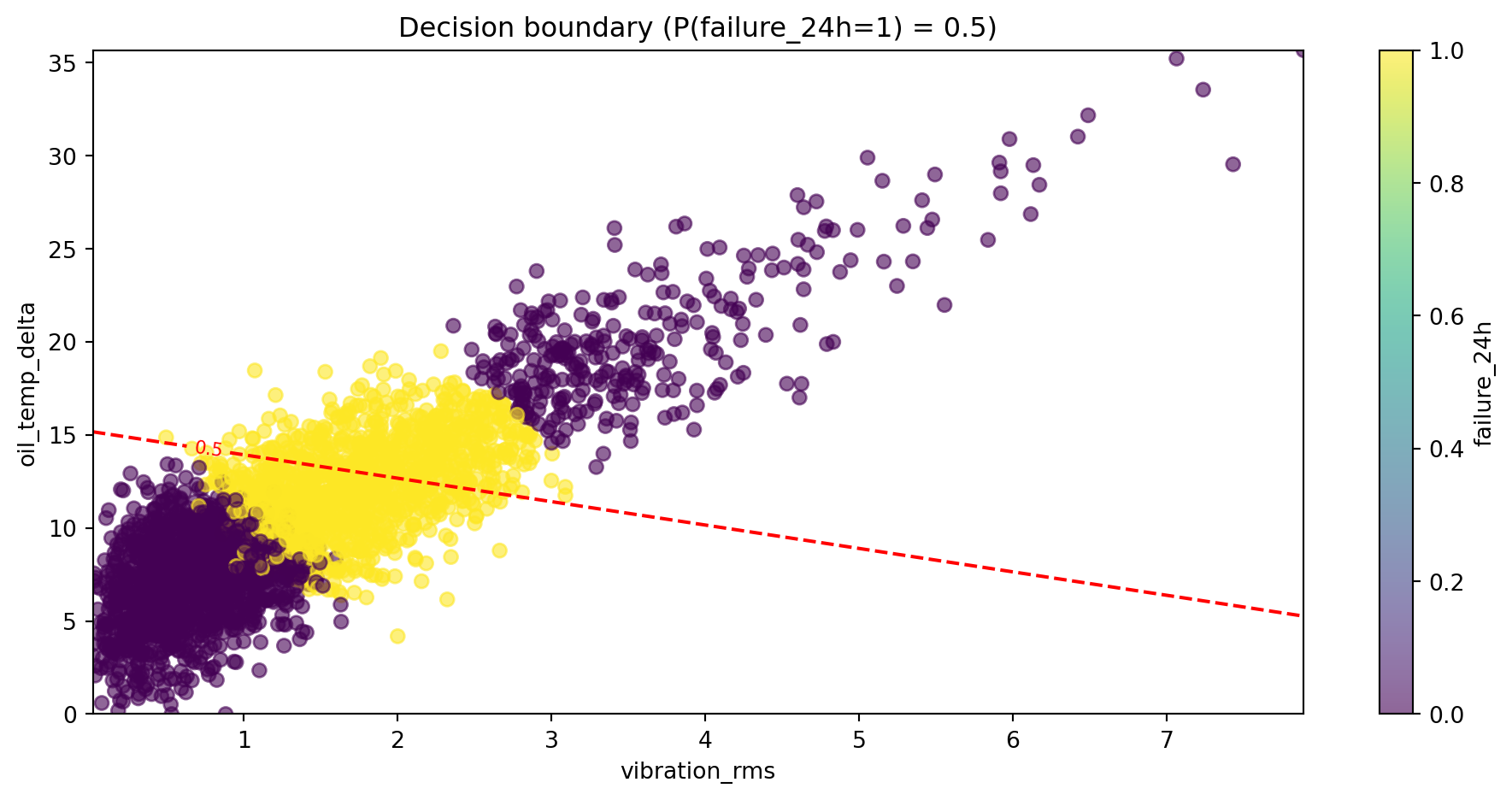
The red dashed line shows where the model is undecided (\(P=0.5\)).
Points on one side are mostly predicted active; on the other, inactive.

Stretch: 3D probability surface (interactive)

import plotly.graph_objects as go

x0 = np.linspace(df["vibration_rms"].min(), df["vibration_rms"].max(), 50)
x1 = np.linspace(df["oil_temp_delta"].min(), df["oil_temp_delta"].max(), 50)
xx, yy = np.meshgrid(x0, x1)
grid = np.c_[xx.ravel(), yy.ravel()]
grid_probs = log_reg.predict_proba(grid)[:, 1].reshape(xx.shape)

surface_fig = go.Figure(
    data=[
        go.Surface(
            x=x0,
            y=x1,
            z=grid_probs,
            colorbar_title="P(active)",
        )
    ]
)

surface_fig.update_layout(
    title="Probability surface P(failure_24h=1)",
    scene=dict(
        xaxis_title="vibration_rms",
        yaxis_title="oil_temp_delta",
        zaxis_title="P(failure_24h=1)",
    )
)

surface_fig.show()

Thresholds and metrics

from sklearn.metrics import confusion_matrix, ConfusionMatrixDisplay

def evaluate_threshold(threshold):
    y_pred = (test_probs_lr >= threshold).astype(int)
    cm = confusion_matrix(y_test_c, y_pred)
    disp = ConfusionMatrixDisplay(cm, display_labels=["inactive", "active"])
    disp.plot(values_format="d")
    plt.title(f"Confusion matrix at threshold={threshold:.2f}")
    plt.tight_layout()
    plt.show()
    acc = accuracy_score(y_test_c, y_pred)
    print(f"Accuracy at threshold={threshold:.2f}: {acc:.3f}")

evaluate_threshold(0.5)

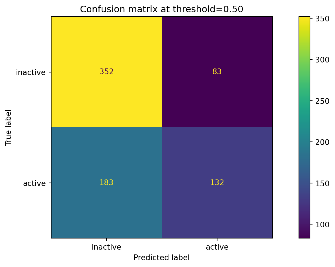
Accuracy at threshold=0.50: 0.645

Now try:

evaluate_threshold(0.3)

and observe how the confusion matrix and accuracy change.

• Lower thresholds usually increase recall for the positive class (more engines flagged).
  
• But they may decrease precision and overall accuracy.

Evaluation: which metrics matter?

In this early-warning system:

• False negative: we miss an at-risk engine (no inspection).
  
• False positive: we unnecessarily inspect a ‘healthy’ engine.

Trade-offs:

• We might accept more false positives (extra inspections) to reduce false negatives (missed at-risk engines).
• Metrics like recall for the at-risk class, along with log-loss and calibration, are more informative than raw accuracy.

Where this idea shows up in practice

Logistic regression (and its generalizations) underpins many real systems:

• Ad click prediction (probability of click on an ad).
• Email spam filters (probability of spam vs not spam).
• Risk scoring (e.g., credit default, failure, medical risk).
• As the final output layer in many neural networks: sigmoid + cross-entropy.

Open questions / research directions:

• How to keep probabilities calibrated in over-parameterized models.
• How to make logistic-type models robust to distribution shift and feedback loops.

Quick checks

1. Why is logistic regression better suited than linear regression for 0/1 labels?

   A. It’s faster to train.
   B. It outputs values in [0,1] and models probabilities directly.
   C. It can’t overfit.
   D. It doesn’t need a train/test split.

2. The logistic loss for a positive example (\(y=1\)) is:

   A. \(-\log(1-\hat{p})\)
   B. \(-\log(\hat{p})\)
   C. \(\hat{p} - y\)
   D. \((\hat{p} - y)^2\)

3. The gradient of the logistic loss w.r.t. $ heta$ for one example is proportional to:

   A. \((y - \hat{p}) x\)
   B. \((\hat{p} - y) x\)
   C. \(x\)
   D. \(y x\)

4. In our student-engagement example, which metric is most aligned with the decision to flag at-risk engines?

   A. Overall accuracy.
   B. Recall for the at-risk (inactive) class.
   C. Number of parameters in the model.
   D. Training set size.