M57: Algorithmic bias & fairness frames

CSCI 1109 — Practical Data Science

Frank Rudzicz

Table of contents

• Conceptual scaffold
• Math lens
• Worked examples
• Summary

Learning outcomes

By the end of this module, you should be able to:

• Explain three sources of algorithmic bias (data, model, feedback loops) and give a real-world example of each.
• Define and compute three fairness metrics — demographic parity, equalized odds, and predictive parity — from a confusion matrix.
• Articulate the impossibility result: why no classifier can satisfy all three metrics simultaneously when base rates differ.
• Audit a simple sklearn classifier for fairness across a protected attribute using Python.
• Evaluate which fairness frame is most appropriate for a given decision context, and justify the tradeoffs.

Conceptual scaffold

What is algorithmic bias?

Algorithmic bias is a systematic and unfair skew in a model’s outputs that disadvantages certain groups, based on race, gender, age, disability, or other characteristics.

Key word: systematic. Random errors are noise. Bias is a consistent pattern.

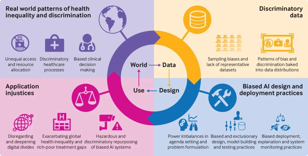
How bias amplifies

From Fusar-Poli et al. (2022).

1. Data bias — the training set reflects historical inequities.
2. Model/design bias — proxy features silently encode protected attributes; loss functions optimise globally, ignoring subgroup harm.
3. Feedback loops — biased decisions produce biased new data, amplifying the problem over time.

Not all bias is illegal or even (always) wrong — a spam filter should be biased against phishing emails, e.g..

The hard question: which systematic errors are acceptable, for whom, and who decides?

Real examples 😔

🧠 Bias type	🛠️ System	💡 What happened
🧑🏿 Racial proxy	COMPAS 🔗 ProPublica	Recidivism scores were twice as likely to false-flag Black defendants as high-risk
👩 Gender	Amazon hiring tool (Dastin 2018)	Résumé ranker penalised CVs containing the word “women’s”
👴 Age	🔗iTutorGroup AI	Auto-rejected applicants over a certain age; $365K settlement
🩺 Racial proxy	Healthcare algorithm (Obermeyer et al. 2019)	Used healthcare spending as a proxy for need — but spending correlates with race/income
📷 Gender × race	Facial recognition (Buolamwini and Gebru 2018)	Error rates up to 35% for dark-skinned women vs <1% for light-skinned men

All of these systems had high overall accuracy. Aggregate metrics hid subgroup failures.

Anti-example 🚨 “It’s fine — we removed the protected attribute”

Anti-example: fairness through unawareness

A data science team builds a loan approval model.
They reason: “We removed race from the features — the model can’t be biased.”

Why this fails:

• Proxy variables. Zip code, school name, or “years at current address” can encode race or socioeconomic status strongly enough to reconstruct it.
• Historical data. If past loans were approved at different rates for different groups, the model learns those patterns even without an explicit protected feature.
• Disparate impact. U.S. law (and common sense ethics) evaluates outcomes, not just inputs. A “race-blind” model that approves white applicants at 3× the rate of equally qualified Black applicants is still discriminatory.

Moral of the story:
Removing a sensitive column is a necessary but far-from-sufficient step.
You must measure outcomes by group.

Math lens

The setup: a binary classifier

Suppose we have:

• A protected attribute \(A \in \{0, 1\}\) (e.g., group \(A=0\) vs \(A=1\)).
• A true label \(Y \in \{0, 1\}\) (e.g., repaid loan = 1).
• A model prediction \(\hat{Y} \in \{0, 1\}\).

We can compute a confusion matrix for each group separately:

	Predicted 1	Predicted 0
True 1	TP	FN
True 0	FP	TN

From these, we derive:

• TPR (True Positive Rate / Recall) \(= \frac{TP}{TP+FN}\)
• FPR (False Positive Rate) \(= \frac{FP}{FP+TN}\)
• PPV (Positive Predictive Value / Precision) \(= \frac{TP}{TP+FP}\)

👉 Three fairness frames ask: which of these should be equal across groups?

🖼️ Frame 1: Demographic parity

Demographic parity (also: statistical parity, equal selection rate):

\[ P(\hat{Y}=1 \mid A=0) = P(\hat{Y}=1 \mid A=1) \]

Both groups (\(A\)) are approved (\(\hat{Y}\); or flagged, or hired) at the same rate, regardless of the true label.

When it makes sense:

• You believe the opportunity itself should be distributed equally (e.g., who gets shown a job ad).
• Historical base-rate differences reflect past discrimination rather than genuine capability differences.

When it’s problematic:

• If the groups genuinely differ in the relevant outcome (e.g., a medical test for a disease that affects one group more), forcing equal positive rates distorts clinical care.

Tip

✏️ Think (and write): a university that accepts students at the same rate from every school district, regardless of grades — is that fair?
(Depends entirely on why grades differ between districts.)

🖼️ Frame 2: Equalized odds

Equalized odds (Hardt, Price, and Srebro 2016):

\[ P(\hat{Y}=1 \mid Y=y, A=0) = P(\hat{Y}=1 \mid Y=y, A=1) \quad \text{for } y \in \{0,1\} \]

Equivalently: both TPR and FPR are equal across groups.

Among people who truly qualify (Y=1), both groups are approved at the same rate.
Among people who truly don’t (Y=0), both groups are falsely approved at the same rate.

Strengths:

• Respects the true label — you’re not penalizing one group for having a higher base rate.
• Directly captures the most common discrimination concern: equally qualified people should be treated equally.

In the COMPAS context:

• COMPAS failed equalized odds: it had a higher false positive rate for Black defendants (labelling truly low-risk people as high-risk).

🖼️ Frame 3: Predictive parity (calibration)

Predictive parity (also: calibration by group):

\[ P(Y=1 \mid \hat{Y}=1, A=0) = P(Y=1 \mid \hat{Y}=1, A=1) \]

Among people that the model predicts will succeed (or re-offend), the same fraction actually does — in both groups.

Strengths:

• Ensures model scores mean the same thing regardless of group — important for trust and for decision-makers who take the score at face value.
• Northpointe (COMPAS creators) argued their tool did satisfy this — and they were correct!

The catch:

• As we’re about to see, satisfying calibration while the groups have different base rates forces the false positive rates to differ.

🔬 The impossibility result

Theorem (Chouldechova 2017; Kleinberg, Mullainathan, and Raghavan 2017):

Suppose two groups have different base rates \[ P(Y=1 \mid A=0) \ne P(Y=1 \mid A=1). \]

Then no non-trivial classifier can simultaneously satisfy:

1. Demographic parity
2. Equalized odds (equal FPR and TPR)
3. Predictive parity (calibration)

Why? The three constraints form a system of equations in TP, FP, FN, TN. When base rates differ, satisfying any two forces a violation of the third (unless the model is perfect or completely random).

Visual intuition: Different base rates mean the “starting positions” on the ROC curve differ — you can’t align TPR, FPR, and PPV at the same time.

Note

This is not a software bug to fix.
It is a mathematical fact.
Choosing a fairness frame is a values decision and a technical one.

Worked examples

Example 1 — Computing fairness metrics

import numpy as np
import pandas as pd

# Synthetic confusion matrix data for two groups
# Group 0 (e.g., applicants from region A)
TP0, FN0, FP0, TN0 = 40, 10, 20, 30   # base rate = 50/100 = 50%
# Group 1 (e.g., applicants from region B)
TP1, FN1, FP1, TN1 = 15, 5, 30, 50    # base rate = 20/100 = 20%

def fairness_metrics(TP, FN, FP, TN, name):
    n = TP + FN + FP + TN
    sel_rate  = (TP + FP) / n           # demographic parity measure
    TPR       = TP / (TP + FN)          # equalized odds: TPR
    FPR       = FP / (FP + TN)          # equalized odds: FPR
    PPV       = TP / (TP + FP) if (TP + FP) > 0 else float('nan')  # predictive parity
    acc       = (TP + TN) / n
    return pd.Series({
        "Group": name, "N": n, "Accuracy": round(acc, 3),
        "Selection rate": round(sel_rate, 3),
        "TPR (recall)":   round(TPR, 3),
        "FPR":            round(FPR, 3),
        "PPV (precision)": round(PPV, 3),
    })

df_metrics = pd.DataFrame([
    fairness_metrics(TP0, FN0, FP0, TN0, "Group 0"),
    fairness_metrics(TP1, FN1, FP1, TN1, "Group 1"),
])
df_metrics.set_index("Group")

	N	Accuracy	Selection rate	TPR (recall)	FPR	PPV (precision)
Group
Group 0	100	0.70	0.60	0.80	0.400	0.667
Group 1	100	0.65	0.45	0.75	0.375	0.333

What to notice

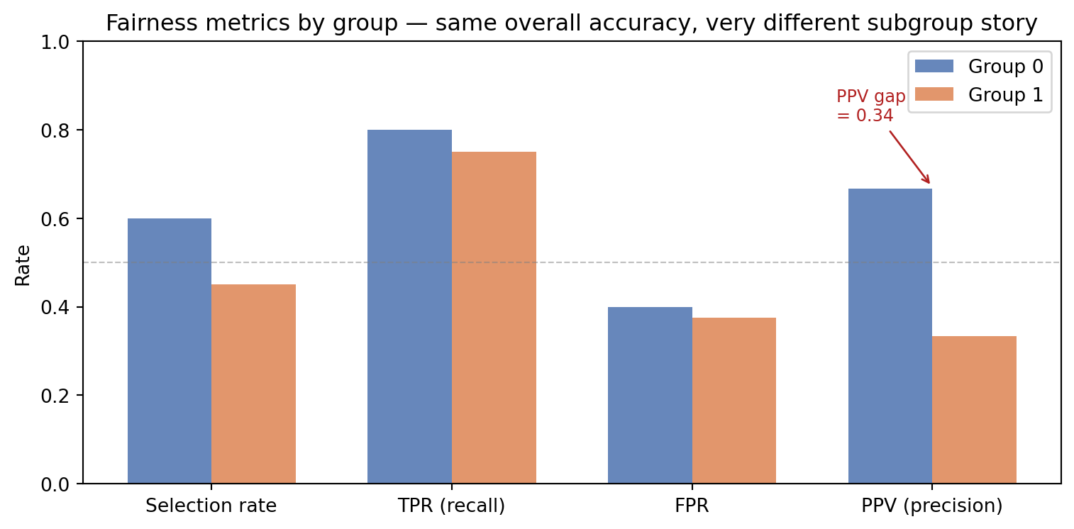
• Overall accuracy looks similar for both groups (~70%).
• Selection rate: Group 0 gets positive decisions at 60%, Group 1 at only 45% — demographic parity is not met.
• TPR: 80% for Group 0 vs 75% for Group 1 — roughly equal.
• FPR: 40% for Group 0 vs 37.5% for Group 1 — nearly equal, so FPR is close to equalized odds.
• PPV: 67% for Group 0 vs 33% for Group 1 — predictive parity is clearly violated.

A data scientist who only reported overall accuracy (~70%) would miss all of this.

Example 1 — Visualization

import matplotlib.pyplot as plt
import matplotlib.patches as mpatches

metrics_to_plot = ["Selection rate", "TPR (recall)", "FPR", "PPV (precision)"]
x = np.arange(len(metrics_to_plot))
width = 0.35

g0_vals = df_metrics.loc[df_metrics["Group"] == "Group 0", metrics_to_plot].values.flatten()
g1_vals = df_metrics.loc[df_metrics["Group"] == "Group 1", metrics_to_plot].values.flatten()

fig, ax = plt.subplots(figsize=(8, 4))
bars0 = ax.bar(x - width/2, g0_vals, width, label="Group 0", color="#4C72B0", alpha=0.85)
bars1 = ax.bar(x + width/2, g1_vals, width, label="Group 1", color="#DD8452", alpha=0.85)

# Highlight PPV disparity
ax.annotate("PPV gap\n= 0.34", xy=(3, 0.67), xytext=(2.6, 0.82),
            arrowprops=dict(arrowstyle="->", color="firebrick"), color="firebrick", fontsize=9)

ax.set_xticks(x)
ax.set_xticklabels(metrics_to_plot, fontsize=10)
ax.set_ylim(0, 1.0)
ax.set_ylabel("Rate")
ax.set_title("Fairness metrics by group — same overall accuracy, very different subgroup story")
ax.legend()
ax.axhline(0.5, color="grey", linestyle="--", linewidth=0.8, alpha=0.5)
plt.tight_layout()
plt.show()

Aggregate accuracy of ~70% hides a PPV gap of 34 percentage points.
Group 1 applicants who are approved are half as likely to actually succeed — the model’s positive label means something different for each group.

Example 2 — Auditing a logistic regression

from sklearn.linear_model import LogisticRegression
from sklearn.preprocessing import StandardScaler
from sklearn.metrics import confusion_matrix
import warnings
warnings.filterwarnings("ignore")

rng = np.random.default_rng(42)
n = 600

# Two groups with different base rates AND different feature signal strengths.
# The weaker signal for Group 1 mimics a common real problem: 
# measurements/proxies were designed/validated primarily on Group 0.
group = rng.integers(0, 2, n)
base_rate     = np.where(group == 0, 0.55, 0.30)
signal        = np.where(group == 0, 0.70, 0.25)   # key: weaker signal for Group 1
y             = rng.binomial(1, base_rate)

x1 = rng.normal(signal * y, 1.0)
x2 = rng.normal(signal * y * 0.8, 1.0)
X  = np.column_stack([x1, x2])

# Train on features ONLY (group not included — "fair by unawareness")
scaler  = StandardScaler()
X_sc    = scaler.fit_transform(X)
model   = LogisticRegression()
model.fit(X_sc, y)
y_pred  = model.predict(X_sc)

# Audit by group
rows = []
for g in [0, 1]:
    mask = group == g
    tn, fp, fn, tp = confusion_matrix(y[mask], y_pred[mask]).ravel()
    n_g = mask.sum()
    rows.append({
        "Group": f"Group {g}",
        "N": int(n_g),
        "Base rate": round(y[mask].mean(), 3),
        "Selection rate": round(y_pred[mask].mean(), 3),
        "TPR": round(tp/(tp+fn) if tp+fn>0 else 0, 3),
        "FPR": round(fp/(fp+tn) if fp+tn>0 else 0, 3),
        "PPV": round(tp/(tp+fp) if tp+fp>0 else 0, 3),
    })

df_audit = pd.DataFrame(rows).set_index("Group")
df_audit

	N	Base rate	Selection rate	TPR	FPR	PPV
Group
Group 0	304	0.530	0.391	0.584	0.175	0.790
Group 1	296	0.297	0.243	0.307	0.216	0.375

Design choice — two compounding problems

group was never given to the model, yet two fairness violations appear:

1. Unequal TPR — Group 1’s positive examples have weaker feature signal (e.g., because the measurements were designed or standardised mainly on Group 0). The model catches far fewer of Group 1’s true positives.
2. Unequal PPV — Because the base rate is lower and the signal is weaker, a positive prediction for Group 1 is less reliable than for Group 0.

Both problems arise without any explicitly “unfair” coding decision. A fairness audit is the only way to see them.

Example 2 — Visualizing the audit

fig, axes = plt.subplots(1, 2, figsize=(10, 4), sharey=False)

# Left: bar chart of rates
cols = ["Base rate", "Selection rate", "TPR", "FPR", "PPV"]
x_pos = np.arange(len(cols))
width = 0.35
g0 = df_audit.loc["Group 0", cols].values
g1 = df_audit.loc["Group 1", cols].values

axes[0].bar(x_pos - width/2, g0, width, label="Group 0", color="#4C72B0", alpha=0.85)
axes[0].bar(x_pos + width/2, g1, width, label="Group 1", color="#DD8452", alpha=0.85)
axes[0].set_xticks(x_pos)
axes[0].set_xticklabels(cols, rotation=20, ha="right", fontsize=9)
axes[0].set_ylim(0, 1)
axes[0].set_title("Fairness audit: group 0 vs group 1")
axes[0].legend(fontsize=9)

# Right: scatter of TPR vs FPR for each group
axes[1].scatter(df_audit["FPR"], df_audit["TPR"],
                c=["#4C72B0", "#DD8452"], s=150, zorder=5)
for g in df_audit.index:
    axes[1].annotate(g,
        (df_audit.loc[g, "FPR"] + 0.01, df_audit.loc[g, "TPR"] - 0.025),
        fontsize=9)
axes[1].plot([0,1],[0,1], "k--", alpha=0.3)  # random classifier line
axes[1].set_xlabel("FPR")
axes[1].set_ylabel("TPR")
axes[1].set_title("ROC positions by group")
axes[1].set_xlim(-0.05, 1.0)
axes[1].set_ylim(-0.05, 1.05)

plt.tight_layout()
plt.show()

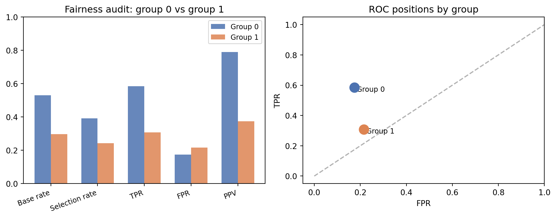
• Group 1 sits lower and to the right on the ROC plot — TPR of 0.295 vs 0.584 for Group 0, and a higher FPR (0.216 vs 0.175).
• Despite per-group accuracies of 0.639 and 0.697 that look broadly similar, the model catches barely 1 in 3 of Group 1’s true positives while catching nearly 3 in 5 of Group 0’s.
• Equalized odds is clearly violated.
• The PPV gap (0.366 vs 0.790) means a positive prediction carries very different weight depending on which group the applicant belongs to — the model’s output doesn’t mean the same thing for everyone.

Summary

Whose fairness counts?

Risk: Framing determines who is harmed

Different fairness frames protect different parties:

Frame	Protects	Penalizes
Demographic parity	Groups with lower opportunity	Groups with genuinely different outcomes
Equalized odds	People who truly qualify	Overall accuracy
Predictive parity	Trust in the score itself	Groups with lower base rates

Choosing a frame is a policy decision, not just a ML one.
It should involve affected communities, domain experts, and legal review — not just the data team.

Simple mitigations:

• Report disaggregated metrics in every model card or deployment summary.
• Require a fairness audit before deployment in high-stakes settings (credit, hiring, healthcare, criminal justice).
• Challenge the task framing: sometimes the fairest intervention is not deploying a model at all, but rather fixing the data-generating process upstream.

Feedback loops & dynamic harm

Risk: Feedback loops compound initial disparities

Many ML systems are not deployed once and frozen.
They produce decisions → those decisions generate new data → the model retrains on that data.

Predictive policing example:

1. Model trained on historical crime data predicts high-crime zones.
2. Police patrol those zones more heavily.
3. More arrests recorded there (because more policing).
4. Model retrained → same zones predicted as high-risk, but now with more training evidence.
5. Under-policed areas appear safer — not because they are, but because no one is looking.

Mitigation strategies (appropriate for this course level):

• Audit model outputs periodically, not just at launch.
• Use causal thinking: ask “would a change in group membership, all else equal, change the prediction?” (counterfactual fairness).
• Prefer human-in-the-loop designs for consequential decisions — models should inform, not fully automate.

Where this goes next: fairness toolkits

What you’ve learned here is the foundation for a growing ecosystem of real tools:

Tool	What it does
🔗 Fairlearn	Computes fairness metrics; mitigation algorithms (e.g., threshold optimization, reductions)
🔗 IBM AI Fairness 360	Broad suite of bias metrics and pre/in/post-processing mitigations
SHAP	Explains individual predictions — useful for spotting proxy variables
Model cards (Mitchell et al. 2019)	Standardized documentation format including disaggregated performance

In future courses (e.g., a Responsible AI elective or ML course), you will encounter post-processing methods like equalized odds post-processing and algorithmic techniques like adversarial debiasing that go beyond threshold tuning.

Bigger picture: data science as a social act

The models you build will likely be trained on data about people.
Deploying them will affect people.

Note

The same Python skills — groupby, .mean(), confusion matrices — that you used for exploratory analysis are the exact tools for a fairness audit.

You already know how to do this. The question is whether you choose to.

Three questions worth asking before deploying any classifier:

1. Who is in my training data — and who is missing?
2. What does my model’s error cost, and for whom?
3. Who benefits if the model is wrong in a particular direction?

These questions are cheap to ask and expensive to ignore.

Quick checks

Q1: A credit scoring model achieves 85% accuracy on both Group A and Group B.
A fairness audit reveals that the False Positive Rate for Group B is 28%, compared with 8% for Group A.

Which fairness criterion is violated?

A. Demographic parity
B. Equalized odds
C. Predictive parity
D. None — equal accuracy means the model is fair

---

Q2: A team building a hiring model removes the gender column from the feature set.
A colleague argues: “The model is now fair by design.”

Which of the following is the strongest counter-argument?

A. Removing a feature always reduces accuracy, which is itself a form of bias.
B. Other features (e.g., job title gaps, university name) may correlate with gender and act as proxies.
C. The model cannot be fair unless it achieves equal accuracy on all demographic groups.
D. Only legally protected attributes need to be removed, and gender is not always protected.

---

Q3: Group X has a loan repayment base rate of 70%. Group Y has a base rate of 30%.
A calibrated model (satisfying predictive parity) assigns the same predicted probability to all applicants.

Without any other changes, which outcome is mathematically guaranteed?

A. Demographic parity is automatically satisfied.
B. Equalized odds (equal TPR and FPR) is automatically satisfied.
C. At least one of TPR or FPR must differ between the groups.
D. The model must also satisfy demographic parity or equalized odds once it is calibrated.

---

Q4: You are building a diagnostic screening tool for a rare disease (base rate ≈ 2%).
The disease is treatable if caught early, but treatment has significant side effects.

Which fairness frame is most important to prioritize, and why?

A. Demographic parity — the same fraction of each group should test positive.
B. Equalized odds — people who truly have the disease should be detected at the same rate, and healthy people should be falsely alarmed at the same rate across groups.
C. Predictive parity — a positive test result should have the same meaning (probability of true disease) for every group.
D. Overall accuracy — minimizing total misclassifications is the dominant concern at 2% base rate.

References

Buolamwini, Joy, and Timnit Gebru. 2018. “Gender Shades: Intersectional Accuracy Disparities in Commercial Gender Classification.” In Proceedings of the 1st Conference on Fairness, Accountability and Transparency (FAccT), 81:77–91. Proceedings of Machine Learning Research. PMLR.

Chouldechova, Alexandra. 2017. “Fair Prediction with Disparate Impact: A Study of Bias in Recidivism Prediction Instruments.” Big Data 5 (2): 153–63. https://doi.org/10.1089/big.2016.0047.

Dastin, Jeffrey. 2018. “Amazon Scraps Secret AI Recruiting Tool That Showed Bias Against Women.” Reuters. https://www.reuters.com/article/us-amazon-com-jobs-automation-insight-idUSKCN1MK08G.

Fusar-Poli, Paolo, Mirko Manchia, Nikolaos Koutsouleris, David Leslie, Christiane Woopen, Monica E. Calkins, Michael Dunn, et al. 2022. “Ethical Considerations for Precision Psychiatry: A Roadmap for Research and Clinical Practice.” European Neuropsychopharmacology 63 (October): 17–34. https://doi.org/10.1016/j.euroneuro.2022.08.001.

Hardt, Moritz, Eric Price, and Nathan Srebro. 2016. “Equality of Opportunity in Supervised Learning.” In Advances in Neural Information Processing Systems (NeurIPS), 29:3315–23.

Kleinberg, Jon, Sendhil Mullainathan, and Manish Raghavan. 2017. “Inherent Trade-Offs in the Fair Determination of Risk Scores.” In Proceedings of the 8th Innovations in Theoretical Computer Science Conference (ITCS). Schloss Dagstuhl–Leibniz-Zentrum für Informatik. https://doi.org/10.4230/LIPIcs.ITCS.2017.43.

Mitchell, Margaret, Simone Wu, Andrew Zaldivar, Parker Barnes, Lucy Vasserman, Ben Hutchinson, Elena Spitzer, Inioluwa Deborah Raji, and Timnit Gebru. 2019. “Model Cards for Model Reporting.” In Proceedings of the Conference on Fairness, Accountability, and Transparency, 220–29. https://doi.org/10.1145/3287560.3287596.

Obermeyer, Ziad, Brian Powers, Christine Vogeli, and Sendhil Mullainathan. 2019. “Dissecting Racial Bias in an Algorithm Used to Manage the Health of Populations.” Science 366 (6464): 447–53. https://doi.org/10.1126/science.aax2342.