M50: Clustering with k-Means; scaling effects
CSCI 1109 — Practical Data Science
Silhouette score
how separated are the clusters?
So far we’ve looked at k-means geometry and some sanity checks.
The silhouette score is an internal metric that tries to answer:
For each point, am I closer to my own cluster than to any other cluster?
For a given point \(i\):
- Let \(a(i)\) be the average distance from \(i\) to all other points in the same cluster.
- Let \(b(i)\) be the smallest average distance from \(i\) to any other cluster.
Then we compare \(a(i)\) vs \(b(i)\):
- If \(a(i)\) is much smaller than \(b(i)\):
\(\Rightarrow\) \(i\) is tightly inside its own cluster, far from others. - If \(a(i) \approx b(i)\):
\(\Rightarrow\) \(i\) is near a boundary between clusters. - If \(a(i) > b(i)\):
\(\Rightarrow\) \(i\) is (on average) closer to another cluster than its own.
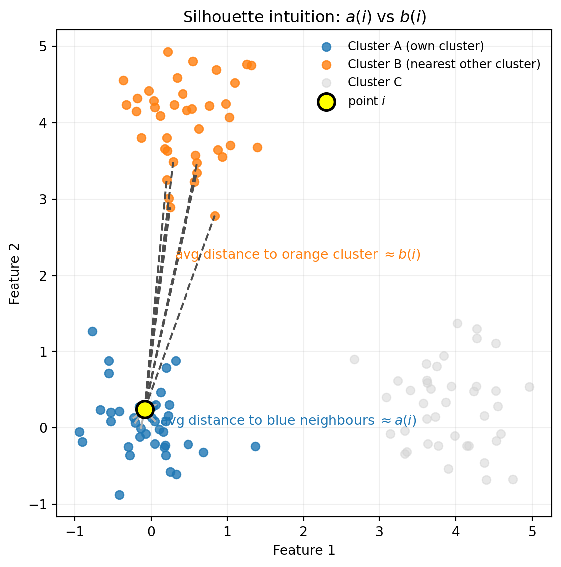
a(i) ≈ 0.55, b(i) ≈ 3.81\(k\)-means without scaling
Code
| annual_spend | visits_per_month | |
|---|---|---|
| cluster_raw | ||
| 0 | 1495.0 | 4.0 |
| 1 | 2996.6 | 5.8 |
| 2 | 500.4 | 1.9 |
Now plot:
Code
fig, ax = plt.subplots()
scatter = ax.scatter(
    customers["annual_spend"],
    customers["visits_per_month"],
    c=customers["cluster_raw"]
)
centers = kmeans_raw.cluster_centers_
ax.scatter(centers[:, 0], centers[:, 1], marker="X", s=200, edgecolor="black")
ax.set_xlabel("Annual spend ($)")
ax.set_ylabel("Visits per month")
ax.set_title("k-means on raw features")
plt.show()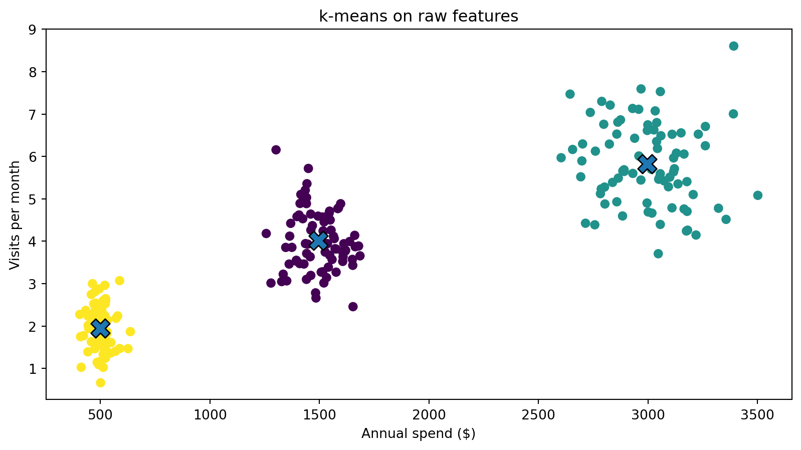
Note
This looks okay because our features were designed nicely.
k-means with distorted scaling
Suppose we accidentally record:
annual_spendin thousands of dollars;visits_per_monthunchanged.
Now annual_spend has much smaller numerical range.
Code
customers_bad = customers.copy()
customers_bad["annual_spend_k"] = customers_bad["annual_spend"] / 1000

kmeans_bad = KMeans(n_clusters=3, n_init=10, random_state=1109)
customers_bad["cluster_bad"] = kmeans_bad.fit_predict(
    customers_bad[["annual_spend_k", "visits_per_month"]]
)

customers_bad.groupby("cluster_bad")[["annual_spend_k", "visits_per_month"]].mean().round(2)| annual_spend_k | visits_per_month | |
|---|---|---|
| cluster_bad | ||
| 0 | 2.95 | 6.00 |
| 1 | 0.54 | 1.97 |
| 2 | 1.64 | 4.05 |
Code
fig, ax = plt.subplots()

scatter = ax.scatter(
    customers_bad["annual_spend_k"],
    customers_bad["visits_per_month"],
    c=customers_bad["cluster_bad"]
)
centers_bad = kmeans_bad.cluster_centers_
ax.scatter(centers_bad[:, 0], centers_bad[:, 1], marker="X", s=200, edgecolor="black")
ax.set_xlabel("Annual spend (thousands of $)")
ax.set_xlim(0,9)
ax.set_ylabel("Visits per month")
ax.set_title("k-means with distorted scaling")
plt.show()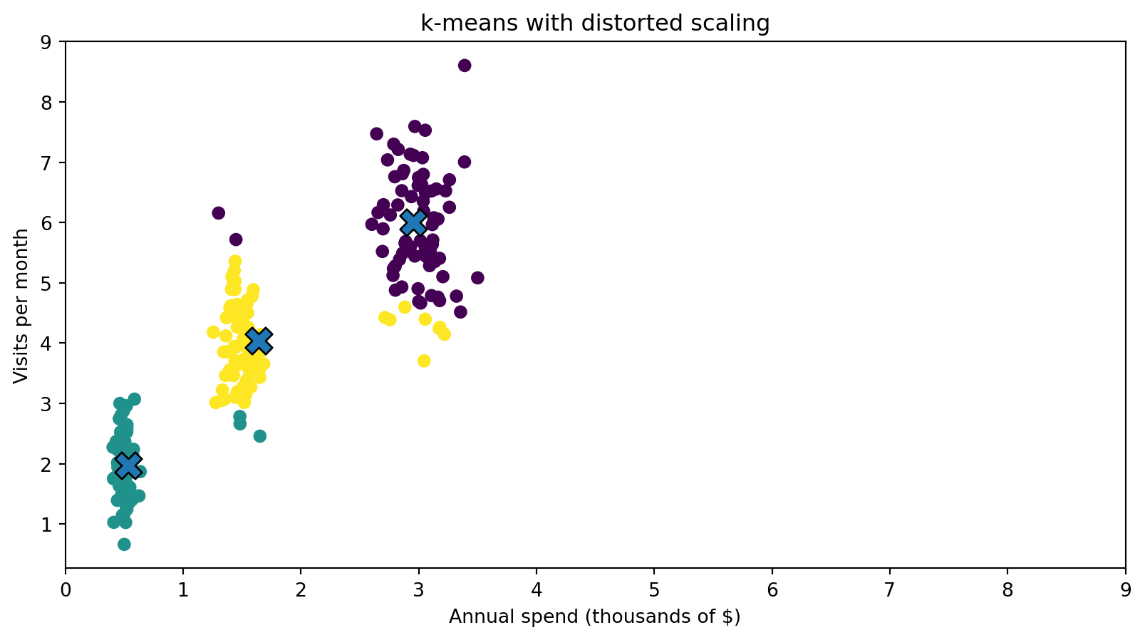
What often happens conceptually
- If one feature’s range is tiny relative to another, distances are dominated by the larger-scale feature.
- Here, distances are mostly about
visits_per_month;annual_spend_kcontributes much less. - Clusters may become horizontal bands (by visits), not meaningful spend–visit groups.
This is why we need feature scaling.
Fixing the geometry with StandardScaler
Code
pipe_scaled = Pipeline([
    ("scaler", StandardScaler()),
    ("kmeans", KMeans(n_clusters=3, n_init=10, random_state=1109))
])

customers["cluster_scaled"] = pipe_scaled.fit_predict(
    customers[["annual_spend", "visits_per_month"]]
)

customers.groupby("cluster_scaled")[["annual_spend", "visits_per_month"]].mean().round(1)| annual_spend | visits_per_month | |
|---|---|---|
| cluster_scaled | ||
| 0 | 1495.0 | 4.0 |
| 1 | 2996.6 | 5.8 |
| 2 | 500.4 | 1.9 |
Code
fig, ax = plt.subplots()
scatter = ax.scatter(
    customers["annual_spend"],
    customers["visits_per_month"],
    c=customers["cluster_scaled"]
)
centers_scaled = pipe_scaled.named_steps["kmeans"].cluster_centers_
# Need to inverse-transform centers back to original scale for plotting:
centers_scaled_orig = pipe_scaled.named_steps["scaler"].inverse_transform(centers_scaled)
ax.scatter(centers_scaled_orig[:, 0], centers_scaled_orig[:, 1],
           marker="X", s=200, edgecolor="black")
ax.set_xlabel("Annual spend ($)")
ax.set_ylabel("Visits per month")
ax.set_title("k-means with standardization")
plt.show()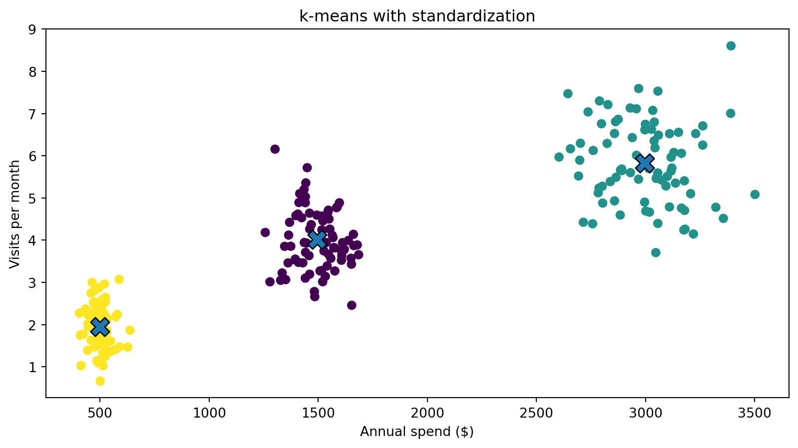
Takeaways
- \(k\)-means is sensitive to feature scales because it uses Euclidean distance.
- Scaling (e.g., standardization) can:
- restore a balanced geometry;
- produce more interpretable, stable clusters.
- In practice: use pipelines with
StandardScalerfor k-means on mixed-scale numeric features.
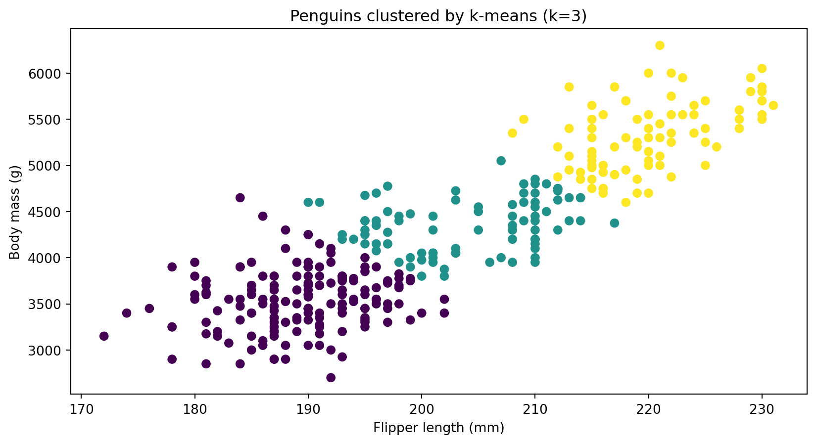
\(k\)-means on penguins (with scaling)
Choosing \(k\)
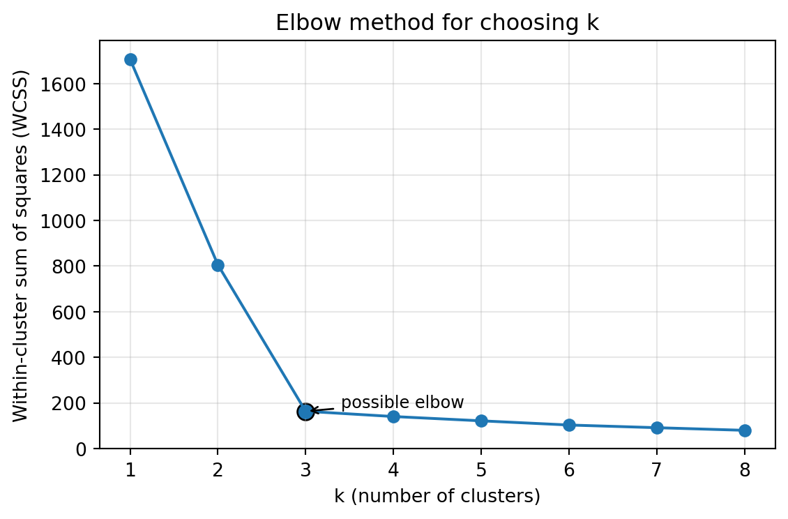
- Common heuristic: elbow method.
- Plot WCSS vs. \(k\); look for a point where improvement slows.
- But: no universally “correct” \(k\); it’s part technical, part judgement.
Code
import numpy as np
import matplotlib.pyplot as plt
from sklearn.cluster import KMeans

# -----------------------------
# Simulate a small 2D dataset
# -----------------------------
rng = np.random.default_rng(1109)

n_per_cluster = 80
centers = np.array([
    [0.0, 0.0],
    [4.0, 0.5],
    [0.5, 4.0]
])

points = []
for cx, cy in centers:
    pts = rng.normal(loc=[cx, cy], scale=[0.6, 0.6], size=(n_per_cluster, 2))
    points.append(pts)

X = np.vstack(points)

# -----------------------------
# Compute WCSS for k = 1..8
# -----------------------------
Ks = range(1, 9)
wcss = []

for k in Ks:
    model = KMeans(n_clusters=k, n_init=20, random_state=1109)
    model.fit(X)
    wcss.append(model.inertia_)  # inertia_ is the WCSS

# -----------------------------
# Plot elbow curve
# -----------------------------
fig, ax = plt.subplots(figsize=(6, 4))

ax.plot(list(Ks), wcss, marker="o")
ax.set_xlabel("k (number of clusters)")
ax.set_ylabel("Within-cluster sum of squares (WCSS)")
ax.set_title("Elbow method for choosing k")
ax.grid(alpha=0.3)

# Optional: annotate a visible elbow around k=3
elbow_k = 3
elbow_wcss = wcss[elbow_k - 1]
ax.scatter([elbow_k], [elbow_wcss], s=80, edgecolor="black")
ax.annotate(
    "possible elbow",
    xy=(elbow_k, elbow_wcss),
    xytext=(elbow_k + 0.4, elbow_wcss * 1.1),
    arrowprops=dict(arrowstyle="->", lw=1),
    fontsize=9,
)

plt.tight_layout()
plt.show()