M47: Logistic regression & error metrics

CSCI 1109 — Practical Data Science

Frank Rudzicz

Table of contents

• Conceptual scaffold
• Math lens
• Worked example 1:
  Simple logistic regression
• Worked example 2:
  Class imbalance & metrics
• Summary

Learning outcomes

By the end of this module, you should be able to:

1. Explain how logistic regression maps feature vectors to probabilities for a binary outcome.
2. Relate the logistic model to linear regression via log-odds and the sigmoid (logistic) function.
3. Implement a simple logistic regression classifier in scikit-learn and interpret its coefficients.
4. Compute and interpret core classification metrics:
   • accuracy, confusion matrix, precision, recall, and F1.
5. Diagnose when accuracy is misleading (e.g., class imbalance) and justify a better metric.
6. Connect model predictions, thresholds, and metrics back to a real decision context (e.g., fraud or health screening).

Conceptual scaffold

Classification vs regression (slight return)

• Regression
  • Target: numeric (e.g., tip percentage, blood pressure).
  • Previous tools: OLS (ordinary least squares) and variants.
  • Evaluation: MAE, RMSE, residual plots, etc.
• Binary classification
  • Target: 2 categories (e.g., sick vs healthy, fraud vs not fraud).
  • We care about:
    • Probabilities: \(\mathbb{P}(Y=1 \mid X)\).
    • Decisions: predict class 1 if probability > threshold (e.g., 0.5).
• Logistic regression is a way to:
  • Take features \(x\) (a vector),
  • Produce a probability \(\hat{p}(y=1 \mid x)\),
  • Turn that into a class prediction via a threshold.

Why not just use linear regression?

Tempting idea:

• Code class labels as \(y \in \{0, 1\}\) and fit linear regression: \[ \hat{y} = w^\top x + b \]
• Interpret \(\hat{y}\) as “probability” and threshold at 0.5.

Problems:

1. Out-of-range predictions:
   • Linear regression can produce \(\hat{y} < 0\) or \(\hat{y} > 1\).
2. Non-linear probability relationship:
   • True probability often changes non-linearly with features.
3. Heteroskedastic errors:
   • The variance of errors is not constant across feature space.
4. Asymmetry of classes and costs:
   • Predicting 0.3 vs 0.7 should not be treated symmetrically if we threshold later.

We want a model that:

• Produces outputs in [0, 1].
• Has a probabilistic interpretation built in.
• Plays nicely with likelihood / log-likelihood.

Logistic regression: high-level picture

Goal: Model the probability that \(y=1\) given features \(x\).

Two key steps:

1. Compute a linear score \(z\): \[ z = w^\top x + b. \]

2. Squash \(z\) into a probability with the sigmoid (logistic) function: \[ \sigma(z) = \frac{1}{1 + e^{-z}}. \]

Then:

• \(\hat{p}(y=1 \mid x) = \sigma(w^\top x + b)\)
• \(\hat{p}(y=0 \mid x) = 1 - \hat{p}(y=1 \mid x)\)

Geometric intuition:

• Like a soft version of a separating hyperplane.
• Close to 0 or 1 far from the decision boundary; uncertain near the boundary.

Sigmoid + decision boundary (sketch)

2D decision surface on the left, sigmoid vs linear score on the right.

❌ Anti-example: abusing probabilities

Scenario:

• Suppose you train a logistic regression model for “hospital readmission in 30 days”.
• You sort patients by predicted probability and label the top 10% as “high risk”.
• A policy-maker says: > “These probabilities are exact. If the model says 0.8, that means exactly 80% of those people will come back.”

Why this is an anti-example of correct interpretation:

• Probabilities are estimates, with uncertainty.
• Calibration matters: 0.8 should mean “in a big group like this, about 80% come back”, not an individual guarantee.
• The model might be mis-specified (missing features, non-linearities, etc).
• If training data were biased, probabilities can systematically over- or under-estimate risk for certain groups.

Takeaway

• Treat probabilities as useful signals, not crystal balls.
• Always connect them back to data quality, model assumptions, and evaluation.

Math lens

🔬 Sigmoid and log-odds

The sigmoid function:

\[ \sigma(z) = \frac{1}{1 + e^{-z}}. \]

If we define \[ \hat{p} = \sigma(w^\top x + b), \] then we can write the odds and log-odds:

• Odds of \(y=1\): \[ \text{odds} = \frac{\hat{p}}{1 - \hat{p}}. \]

• Log-odds: \[ \log \frac{\hat{p}}{1 - \hat{p}} = w^\top x + b. \]

So logistic regression makes the log-odds a linear function of features.

Interpretation

• Each feature’s coefficient \(w_j\) says:
  • How much the log-odds of \(y=1\) change when \(x_j\) increases by 1, holding other features fixed.

Logistic loss (briefly)

Training logistic regression:

• We choose \(w, b\) to make predicted probabilities close to true labels.
• Common approach: maximum likelihood \(\Rightarrow\) minimize logistic loss.

For each example with label \(y \in \{0, 1\}\) and predicted probability \(\hat{p} = \hat{p}(y=1 \mid x)\):

\[ \ell_{ \text{log}}(\hat{p}, y) = -\left( y \log \hat{p} + (1-y) \log (1-\hat{p}) \right). \]

Properties (intuition, no derivation):

• If \(y=1\):
  • Loss is small if \(\hat{p}\) is close to 1.
  • Loss grows large if \(\hat{p}\) is close to 0.
• If \(y=0\):
  • Loss is small if \(\hat{p}\) is close to 0.
  • Loss grows large if \(\hat{p}\) is close to 1.

In practice: - 🔗 sklearn.linear_model.LogisticRegression handles the optimization for us. - We focus on interpretation and evaluation, not gradient formulas.

🔬 Stretch: from linear regression to logistic

Very high-level sketch:

1. For linear regression, we often assume: \[ y = w^\top x + b + \varepsilon,\quad \varepsilon \sim \mathcal{N}(0, \sigma^2). \]
   • Leads naturally to least squares (OLS).
2. For binary \(y\), a normal error model doesn’t fit well:
   • We want \(y \in \{0,1\}\) and probabilities, not continuous noise.
3. Instead, we assume:
   • Given \(x\), \(y\) follows a Bernoulli distribution with parameter \(\hat{p}(x)\).
   • We model \(\hat{p}(x)\) using the logistic function: \[\hat{p}(x) = \sigma(w^\top x + b).\]
4. Maximizing the likelihood of the observed labels under this model:
   • Gives the logistic loss.
   • Makes logistic regression a kind of “generalized linear model” (GLM).

Tip

You don’t need to memorize the derivation – just know that the model is consistent with a familiar probability story.

Worked example 1:
Simple logistic regression

Predicting malignant vs benign tumours

We’ll use a classic dataset from scikit-learn: digitized images of breast tissue, reduced to numeric features like:

• mean radius, texture, perimeter, area,
• measures of smoothness, compactness, symmetry, etc.

Task:

• Each case is labelled as malignant (cancer) or benign.
• We’ll train a logistic regression model to predict malignant vs benign from the features.

We’ll:

1. Load the dataset with load_breast_cancer.
2. Split into training and validation sets.
3. Fit a logistic regression model (with feature scaling).
4. Look at accuracy and the confusion matrix, and talk about false positives vs false negatives.

Code – data and model

import numpy as np
import pandas as pd

from sklearn.datasets import load_breast_cancer
from sklearn.model_selection import train_test_split
from sklearn.preprocessing import StandardScaler
from sklearn.pipeline import Pipeline
from sklearn.linear_model import LogisticRegression
from sklearn.metrics import (
    accuracy_score, confusion_matrix, ConfusionMatrixDisplay
)

# Load dataset as a pandas DataFrame
cancer = load_breast_cancer(as_frame=True)
X = cancer.data          # features
y = cancer.target        # 0 = malignant, 1 = benign
target_names = cancer.target_names  # ["malignant", "benign"]

X.head()

	mean radius	mean texture	mean perimeter	mean area	mean smoothness	mean compactness	mean concavity	mean concave points	mean symmetry	mean fractal dimension	...	worst radius	worst texture	worst perimeter	worst area	worst smoothness	worst compactness	worst concavity	worst concave points	worst symmetry	worst fractal dimension
0	17.99	10.38	122.80	1001.0	0.11840	0.27760	0.3001	0.14710	0.2419	0.07871	...	25.38	17.33	184.60	2019.0	0.1622	0.6656	0.7119	0.2654	0.4601	0.11890
1	20.57	17.77	132.90	1326.0	0.08474	0.07864	0.0869	0.07017	0.1812	0.05667	...	24.99	23.41	158.80	1956.0	0.1238	0.1866	0.2416	0.1860	0.2750	0.08902
2	19.69	21.25	130.00	1203.0	0.10960	0.15990	0.1974	0.12790	0.2069	0.05999	...	23.57	25.53	152.50	1709.0	0.1444	0.4245	0.4504	0.2430	0.3613	0.08758
3	11.42	20.38	77.58	386.1	0.14250	0.28390	0.2414	0.10520	0.2597	0.09744	...	14.91	26.50	98.87	567.7	0.2098	0.8663	0.6869	0.2575	0.6638	0.17300
4	20.29	14.34	135.10	1297.0	0.10030	0.13280	0.1980	0.10430	0.1809	0.05883	...	22.54	16.67	152.20	1575.0	0.1374	0.2050	0.4000	0.1625	0.2364	0.07678

5 rows × 30 columns

Code – train/validation split

# Train/validation split
X_train, X_val, y_train, y_val = train_test_split(
    X, y,
    test_size=0.3,
    random_state=47,
    stratify=y,
)

# Pipeline: scale features, then logistic regression
log_reg = Pipeline(steps=[
    ("scale", StandardScaler()),
    ("model", LogisticRegression(max_iter=2000))
])

log_reg.fit(X_train, y_train)

# Validation predictions
y_val_pred = log_reg.predict(X_val)
acc = accuracy_score(y_val, y_val_pred)

acc

0.9707602339181286

Classification: Confusion matrix

For binary classification with positive class “malignant”:

	Predicted: malignant	Predicted: benign
Actual: malignant	True Positive (TP)	False Negative (FN)
Actual: benign	False Positive (FP)	True Negative (TN)

From these counts:

• Accuracy: \[\text{Acc} = \frac{\color{green}{TP} + \color{green}{TN}}{\color{green}{TP} + \color{green}{TN} + \color{red}{FP} + \color{red}{FN}}\]
• Precision (fraud): \[\text{Prec} = \frac{\color{green}{TP}}{\color{green}{TP} + \color{red}{FP}}\]

• Recall (fraud): \[\text{Rec} = \frac{\color{green}{TP}}{\color{green}{TP} + \color{red}{FN}}\]
• F1 score (harmonic mean): \[F_1 = 2 \cdot \frac{\text{Prec} \cdot \text{Rec}}{\text{Prec} + \text{Rec}}\]

Classification: Confusion matrix

🧠 Intuition:

• Precision: “If we flag something, how often are we right?”
• Recall: “Of all the true malignancies, how many did we catch?”

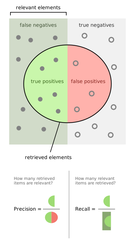
From 🔗 here

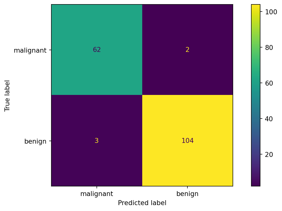
Code – confusion matrix

cm = confusion_matrix(y_val, y_val_pred)

disp = ConfusionMatrixDisplay(
    confusion_matrix=cm,
    display_labels=target_names
)
disp.plot(values_format="d");

Confusion matrix for malignant vs benign classification (threshold 0.5).

Interpreting the confusion matrix

Reading the matrix (with labels [malignant, benign]):

• True Positive (TP) for “malignant”:
  • Predicted malignant, and it really was malignant.
• True Negative (TN):
  • Predicted benign, and it really was benign.
• False Positive (FP):
  • Predicted malignant, but tumour was actually benign
  • ⚠️ unnecessary worry / extra tests.
• False Negative (FN):
  • Predicted benign, but tumour was actually malignant
  • ⚠️ potentially missing a cancer.

✏️ reflection questions:

• In this context, which error is more serious, FP or FN?
• If we wanted to reduce FN (catch more cancers), what might we change?
• Hint: later we’ll see we can adjust the decision threshold (not just stick with 0.5).

Worked example 2:
Class imbalance & metrics

Rare fraud detection (simulated)

Scenario:

• Bank transactions: small fraction are fraudulent.
• Most transactions are legitimate.

Goal:

• Use logistic regression to predict is_fraud (1 = fraud, 0 = not fraud).
• Show why accuracy can be misleading when fraud is rare.
• Introduce precision, recall, and F1.

We’ll simulate a small dataset with:

• Imbalanced classes (~5–10% fraud).
• A few simple, interpretable features.

Code – simulate data

rng = np.random.default_rng(1109)
n = 2000

amount = rng.lognormal(mean=3.0, sigma=1.0, size=n)
is_international = rng.binomial(1, 0.15, size=n)
is_high_risk_country = is_international * rng.binomial(1, 0.3, size=n)
hour = rng.integers(0, 24, size=n)
device_trust = rng.uniform(0, 1, size=n)

# True (hidden) fraud probability model
logit_true = (
    -3.0
    + 0.003 * amount
    + 1.5 * is_international
    + 2.0 * is_high_risk_country
    + 0.02 * (hour - 12)
    - 3.0 * device_trust
)
p_fraud = 1 / (1 + np.exp(-logit_true))
y = rng.binomial(1, p_fraud)

data = pd.DataFrame({
    "amount": amount,
    "is_international": is_international,
    "is_high_risk_country": is_high_risk_country,
    "hour": hour,
    "device_trust": device_trust,
    "is_fraud": y,
})

data["is_fraud"].mean()

0.0415

Code – train logistic regression

from sklearn.metrics import precision_score, recall_score, f1_score

X = data[["amount", "is_international", "is_high_risk_country", "hour", "device_trust"]]
y = data["is_fraud"]

X_train, X_val, y_train, y_val = train_test_split(
    X, y, test_size=0.3, random_state=47, stratify=y
)

log_reg_fraud = LogisticRegression(max_iter=1000)
log_reg_fraud.fit(X_train, y_train)

y_val_pred = log_reg_fraud.predict(X_val)
y_val_proba = log_reg_fraud.predict_proba(X_val)[:, 1]

acc = accuracy_score(y_val, y_val_pred)
prec = precision_score(y_val, y_val_pred, zero_division=0)
rec = recall_score(y_val, y_val_pred, zero_division=0)
f1 = f1_score(y_val, y_val_pred, zero_division=0)

acc, prec, rec, f1

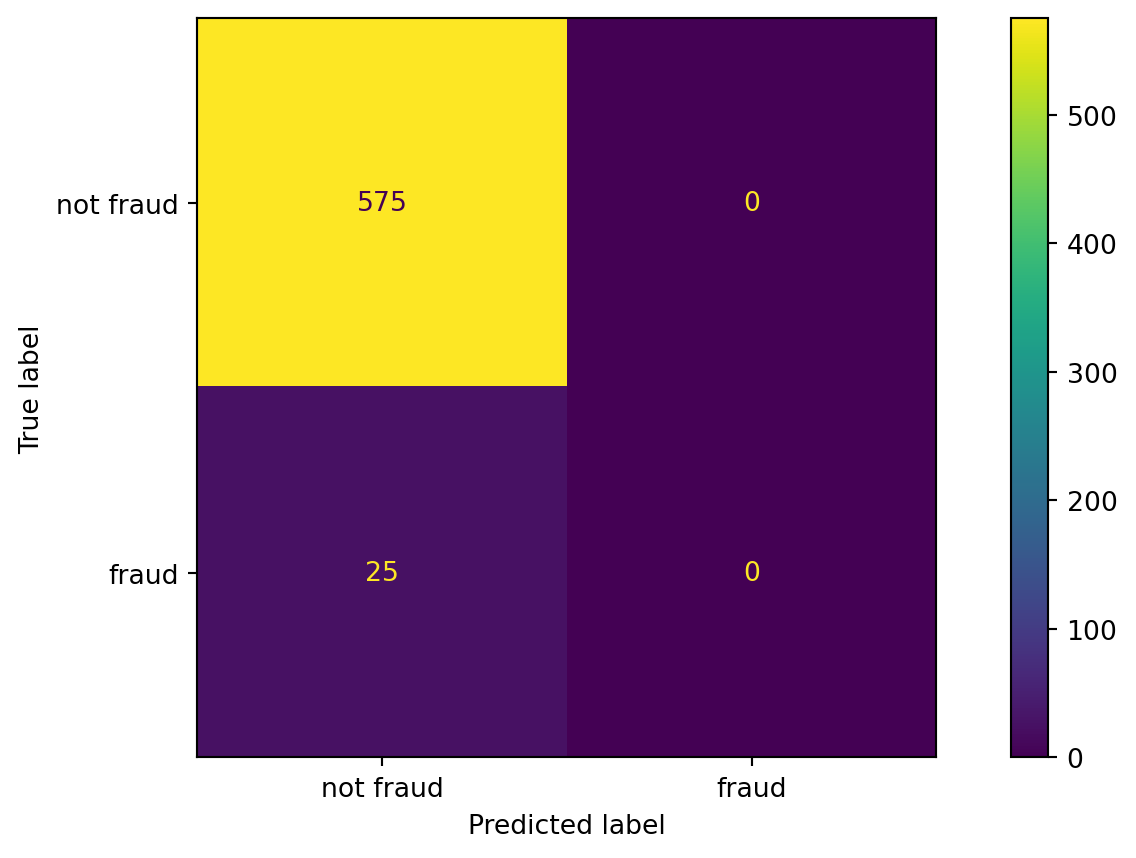
(0.9583333333333334, 0.0, 0.0, 0.0)

Accuracy vs precision / recall

Remember:

• Accuracy: \[ \text{accuracy} = \frac{ \text{TP} + \text{TN}}{ \text{all examples}} \]
  • Can look great when the negative class dominates (e.g., 95% of transactions are legit).
• Precision: \[ \text{precision} = \frac{ \text{TP}}{ \text{TP} + \text{FP}} \]
  • “Of everything we flagged as fraud, how many were actually fraud?”
• Recall: \[ \text{recall} = \frac{ \text{TP}}{ \text{TP} + \text{FN}} \]
  • “Of all the frauds that existed, how many did we catch?”
• F1 score: \[ \text{F1} = 2 \cdot \frac{ \text{precision} \cdot \text{recall}}{ \text{precision} + \text{recall}} \]
  • Harmonic mean; high only if both precision and recall are high.

Code – confusion matrix

cm = confusion_matrix(y_val, y_val_pred)

disp = ConfusionMatrixDisplay(
    confusion_matrix=cm,
    display_labels=["not fraud", "fraud"]
)
disp.plot(values_format="d");

Confusion matrix for malignant vs benign classification (threshold 0.5).

Code – threshold effects

import matplotlib.pyplot as plt

thresholds = np.linspace(0.05, 0.95, 19)
precisions = []
recalls = []

for t in thresholds:
    y_pred_t = (y_val_proba >= t).astype(int)
    precisions.append(precision_score(y_val, y_pred_t, zero_division=0))
    recalls.append(recall_score(y_val, y_pred_t, zero_division=0))

fig, ax = plt.subplots()
ax.plot(thresholds, precisions, marker="o", label="precision")
ax.plot(thresholds, recalls, marker="s", label="recall")
ax.set_xlabel("Decision threshold")
ax.set_ylabel("Metric value")
ax.legend()
ax.set_title("Precision/recall trade-off vs threshold");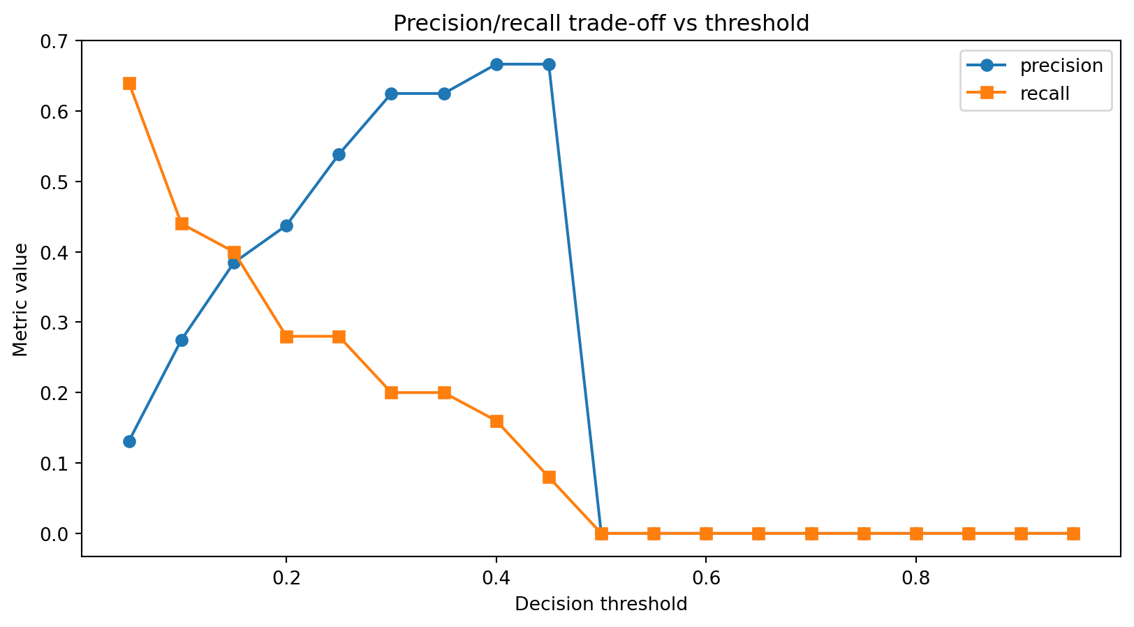

Precision and recall as we vary the decision threshold.

Interpreting the threshold plot

As we increase the threshold:

• We become stricter about calling something “fraud” (need higher probability).
  • Precision tends to go up:
    • Fewer false positives.
  • Recall tends to go down:
    • We miss more true frauds.

As we decrease the threshold:

• We flag more transactions as fraud.
  • Recall usually goes up:
    • We catch more actual fraud.
  • Precision usually goes down:
    • We also annoy more legitimate customers.

Choosing a threshold is a business / policy decision:

• Depends on costs of FP vs FN:
  • FP: blocking legit customers.
  • FN: letting fraud through.

Summary

Loss vs evaluation metric (revisited)

In logistic regression:

• Training objective:
  • Minimize logistic loss (a kind of cross-entropy).
  • Seen by the optimizer during training.
• Evaluation metrics:
  • Accuracy, precision, recall, F1, ROC–AUC, etc.
  • Seen by humans to judge usefulness.

Important

• Loss and metric are related but not identical.
• You might:
  • Train with one loss (e.g., log-loss),
  • Tune threshold or model choices using a different metric (e.g., F1).
• Good practice:
  • Pick metrics that match the decision context and stakeholders.

Connecting back to the pipeline

For a binary classification project in this course, a sensible checklist:

1. Define the decision:
   • Who acts on predictions? What are FP/FN costs?
2. Split the data:
   • Train / validation / (test).
3. Choose baselines:
   • Constant predictor; maybe simple rules.
4. Train a model:
   • Logistic regression, k-NN, etc.
5. Evaluate honestly:
   • Confusion matrix, accuracy, precision, recall, F1.
   • Check class balance and thresholds.
6. Stress-test assumptions:
   • Class imbalance, data leakage, shifts in deployment.
7. Communicate clearly:
   • Explain metrics in words and connect them to real-world trade-offs.

Ethical and practical risks

Using logistic regression + metrics in the real world can go wrong when:

• Class imbalance is extreme:
  • Models look good on paper but rarely catch positive cases (e.g., rare diseases).
• Groups are affected differently:
  • Precision/recall may be much worse for some demographic groups than others.
• Thresholds are chosen carelessly:
  • E.g., “just use 0.5” without thinking about domain costs.
• Data is biased or incomplete:
  • Past decisions baked into the data can mislead the model.

Simple mitigations at our level:

• Always inspect class balance and report it.
• Compute metrics for subgroups where appropriate (e.g., age, region).
• Explore how metrics change across thresholds and explain the trade-offs.
• Document the intended use and limitations of the model in plain language.

Logistic regression in the wild

Where logistic regression shows up:

• Medical risk prediction:
  • Probability of readmission, heart disease, etc.
• Credit scoring:
  • Probability of default.
• Education:
  • Probability of course completion or dropout.
• Social science:
  • Modeling binary outcomes like “vote vs not vote”.

Even in large ML systems:

• Logistic-style layers appear inside modern deep learning models.
• Probabilistic outputs + thresholds are still central to decision-making.

Quick-check questions

1. Conceptual (MCQ)
   You fit a logistic regression model and get \(\hat{p}(y=1 \mid x) = 0.8\) for a patient. Which interpretation is best?

   A. The model is 80% sure this specific patient will definitely get the disease.
   B. If we saw many similar patients, about 80% of them would get the disease.
   C. There is an 80% chance the model is correct.
   D. The patient has exactly 80% of the symptoms.

2. Metrics (short answer)
   A classifier for a rare disease achieves 99% accuracy but 20% recall on the positive class.

   • Explain in one sentence why this might be a bad model for screening.

3. Confusion matrix (numeric)
   Suppose on a small test set you have:

   • TP = 30, FP = 10, FN = 20, TN = 40.

   Compute accuracy, precision, and recall for the positive class.

4. Threshold reasoning (conceptual)
   In a fraud detection system, when might you deliberately choose a lower decision threshold than 0.5?