OLS as orthogonal projection: projecting y onto the column space of X.
CSCI 1109 — Practical Data Science
By the end of this module, you should be able to:
We want a model that predicts a numeric outcome \(y\):
Linear regression says:
“Predict \(y\) as a linear combination of features \(x_1, x_2, \dots, x_p\).”
\[ \hat y = \beta_0 + \beta_1 x_1 + \dots + \beta_p x_p \]
We choose coefficients \(\beta\) to make predictions “close” to the observed \(y\) on the training data.
What does “close” mean? → Least squares: minimize the sum of squared errors.
For \(n\) data points, with \(p\) features:
\[ X = \begin{bmatrix} 1 & x_{11} & x_{12} & \dots & x_{1p} \\ 1 & x_{21} & x_{22} & \dots & x_{2p} \\ \vdots & \vdots & \vdots & \ddots & \vdots \\ 1 & x_{n1} & x_{n2} & \dots & x_{np} \end{bmatrix} \]
Model of reality:
\[ y = X\beta + \varepsilon \]
where:
Ordinary least squares chooses \(\hat\beta\) to minimize squared residuals:
\[ \hat\beta = \arg\min_{\beta} \, \|y - X\beta\|^2 \]
OLS gives one best-fitting vector of predictions \(X\hat\beta\) among all linear combinations of the columns of \(X\).
Key idea: the columns of \(X\) span a subspace of \(\mathbb{R}^n\).
OLS finds the closest point in that subspace to the actual data vector \(y\).
Think of \(\mathbb{R}^n\) as one big space of length-\(n\) vectors (for \(n\) data points):
Now look at all the vectors you can get by taking linear combinations of the columns of \(X\) (things of the form \(X\beta\)).
Those all live together in a flat “sheet” inside \(\mathbb{R}^n\) called the column space of \(X\):
OLS says: “Among all those \(X\beta\) on that sheet, pick the one closest to \(y\) in straight-line distance.”
Note
We have lots of possible straight-line prediction vectors (the plane), and one true outcome vector \(y\). OLS just picks the prediction vector on that plane that’s closest to \(y\), like dropping \(y\) straight down onto the plane and using its shadow.
OLS as orthogonal projection: projecting y onto the column space of X.
We want to choose \(\beta\) to minimize:
\[ L(\beta) = \|y - X\beta\|^2 = (y - X\beta)^\top (y - X\beta) \]
import numpy as np
import matplotlib.pyplot as plt
beta_vals = np.linspace(-3, 3, 200)
# toy 1D quadratic loss: L(β) = (β - 1)^2 + 2
loss = (beta_vals - 1)**2 + 2
plt.plot(beta_vals, loss)
plt.axvline(1, linestyle="--") # true minimizer β* = 1
plt.scatter([1], [2], zorder=3) # point at the bottom
plt.xlabel("β")
plt.ylabel("L(β)")
plt.title("Quadratic 'bowl': minimum where gradient = 0")
plt.tight_layout()
plt.show()
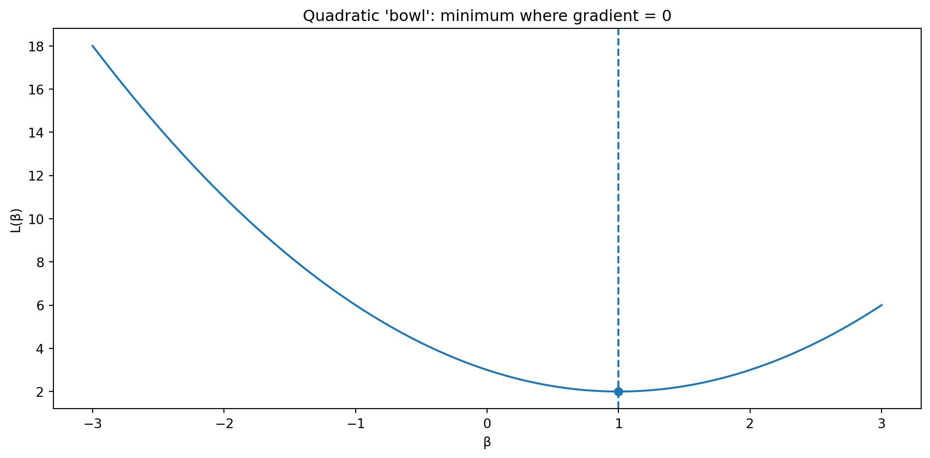
Because \(L(\beta)\) is a smooth quadratic bowl (a convex function of \(\beta\)), its unique minimum is exactly where the gradient is zero, so solving \(\nabla_\beta L(\beta) = 0\) gives us the best \(\hat\beta\).
\[ \nabla_\beta L = -2X^\top(y - X\beta) \]
\[ X^\top y - X^\top X \beta = 0 \]
\[ X^\top X \hat\beta = X^\top y \quad \text{(normal equations)} \]
If \(X^\top X\) is invertible:
\[ \boxed{\hat\beta = (X^\top X)^{-1} X^\top y} \]
From the normal equations:
\[ X^\top (y - X\hat\beta) = 0 \]
Let \(r = y - X\hat\beta\) (residual vector). Then:
\[ X^\top r = 0 \]
Meaning:
Each column of \(X\) is orthogonal to the residual vector.
In other words:
Once you’ve chosen the OLS line/plane, there’s no remaining linear pattern between residuals and any feature in \(X\).
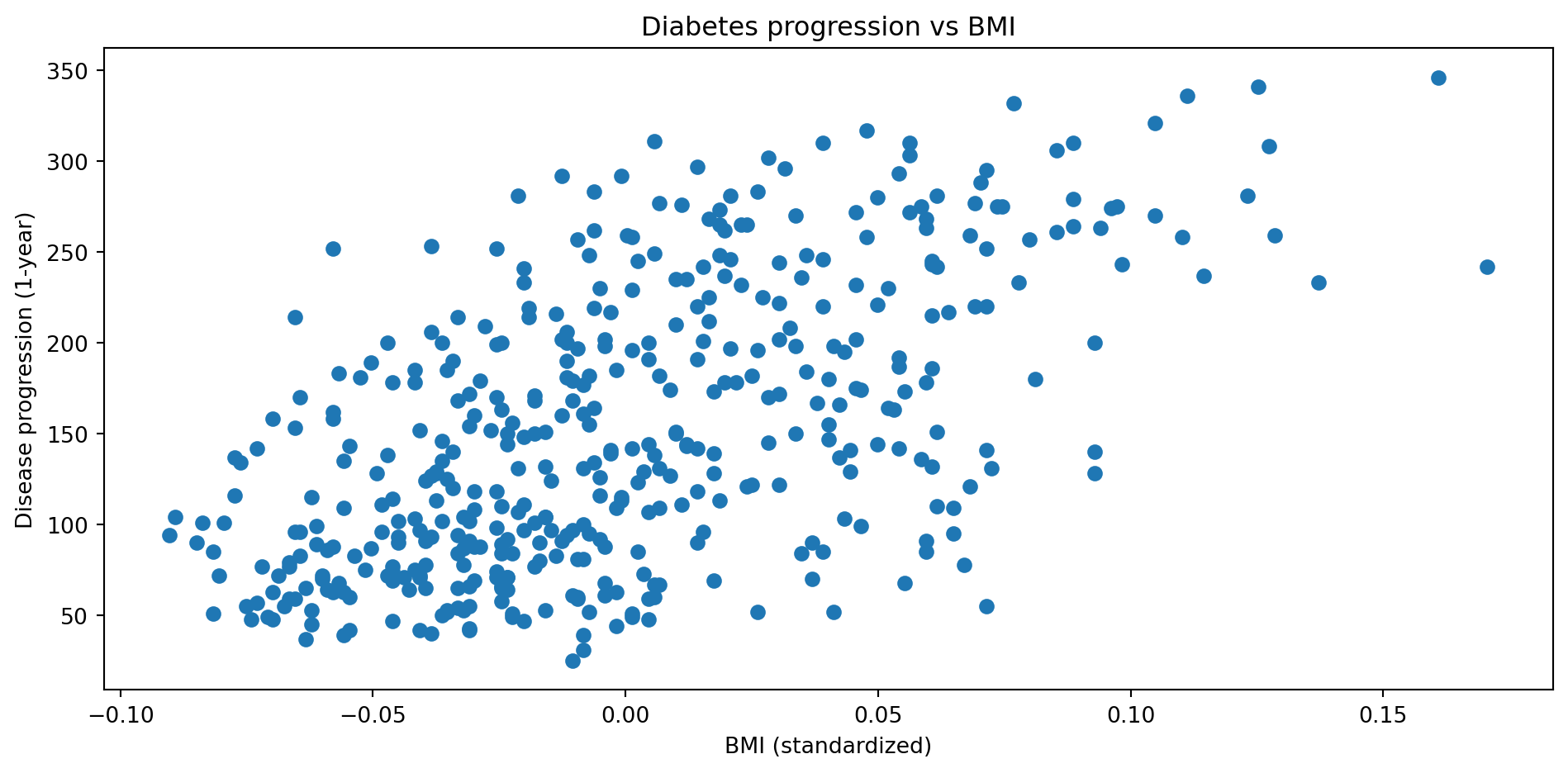
Dataset: classic clinical dataset on diabetes progression.
We’ll start with a simple 1D regression:
Predict disease progression from BMI alone.
import numpy as np
import pandas as pd
import matplotlib.pyplot as plt
from sklearn.datasets import load_diabetes
from sklearn.linear_model import LinearRegression
diab = load_diabetes(as_frame=True)
df_d = diab.frame.copy()
df_d = df_d.rename(columns={"target": "progression"})
df_d[["bmi", "progression"]].head()| bmi | progression | |
|---|---|---|
| 0 | 0.061696 | 151.0 |
| 1 | -0.051474 | 75.0 |
| 2 | 0.044451 | 141.0 |
| 3 | -0.011595 | 206.0 |
| 4 | -0.036385 | 135.0 |
Intercept (beta_0): 152.13348416289617
Slope (beta_1): 949.4352603840372
| age | sex | bmi | bp | s1 | s2 | s3 | s4 | s5 | s6 | progression | pred | |
|---|---|---|---|---|---|---|---|---|---|---|---|---|
| 0 | 0.038076 | 0.050680 | 0.061696 | 0.021872 | -0.044223 | -0.034821 | -0.043401 | -0.002592 | 0.019907 | -0.017646 | 151.0 | 210.710038 |
| 1 | -0.001882 | -0.044642 | -0.051474 | -0.026328 | -0.008449 | -0.019163 | 0.074412 | -0.039493 | -0.068332 | -0.092204 | 75.0 | 103.262195 |
| 2 | 0.085299 | 0.050680 | 0.044451 | -0.005670 | -0.045599 | -0.034194 | -0.032356 | -0.002592 | 0.002861 | -0.025930 | 141.0 | 194.337033 |
| 3 | -0.089063 | -0.044642 | -0.011595 | -0.036656 | 0.012191 | 0.024991 | -0.036038 | 0.034309 | 0.022688 | -0.009362 | 206.0 | 141.124769 |
| 4 | 0.005383 | -0.044642 | -0.036385 | 0.021872 | 0.003935 | 0.015596 | 0.008142 | -0.002592 | -0.031988 | -0.046641 | 135.0 | 117.588574 |
plt.scatter(df_d["bmi"], df_d["progression"], label="Observed")
# Sort for a clean line
order = np.argsort(df_d["bmi"].values)
plt.plot(df_d["bmi"].values[order], df_d["pred"].values[order], label="OLS fit")
plt.xlabel("BMI (standardized)")
plt.ylabel("Disease progression (1-year)")
plt.title("Diabetes progression vs BMI (OLS fit)")
plt.legend()
plt.tight_layout()
plt.show()
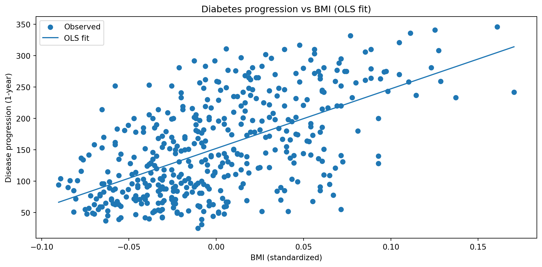
Interpretation

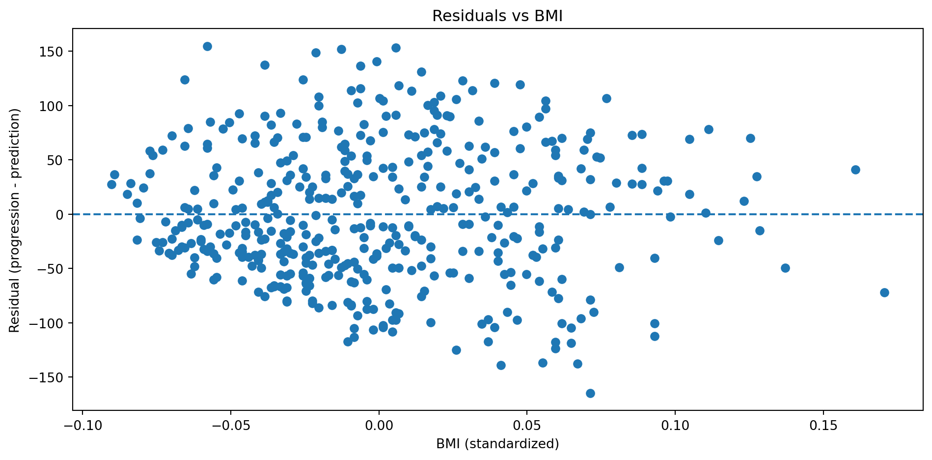
👀 Visual check:

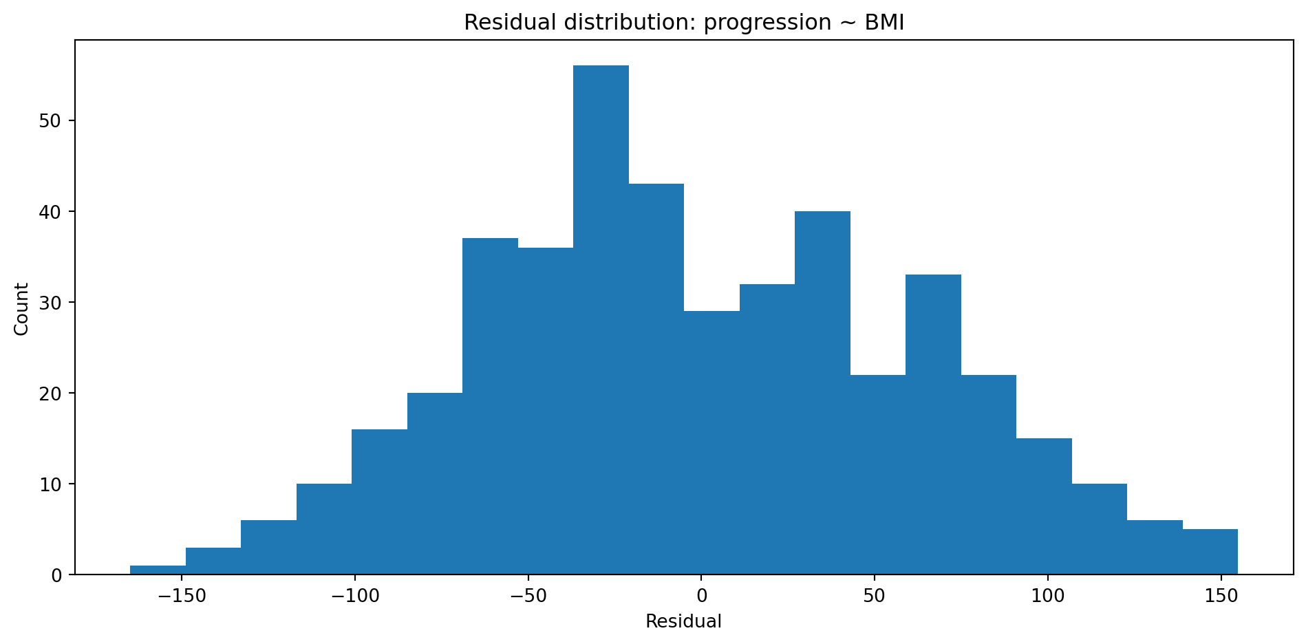
We’re looking for:
This matters more when we want confidence intervals / p-values, less for pure prediction.
In practice, OLS is used when these are at least roughly true:
Plus earlier good practice:
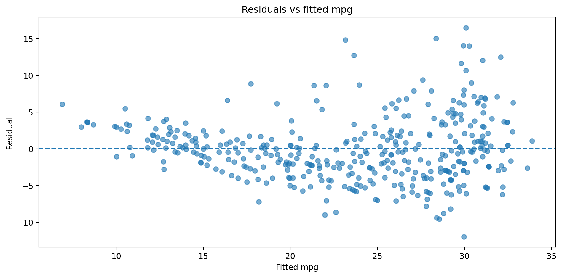
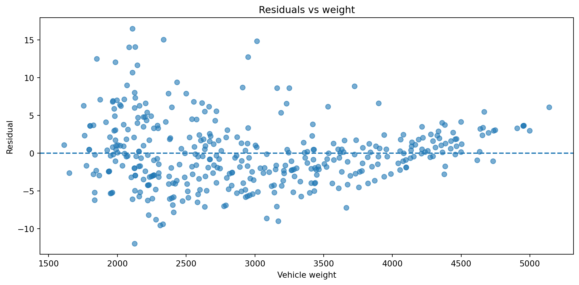
Simple visual diagnostics:
We saw a mostly okay example (progression ~ BMI).
Next: a higher-impact anti-example from energy & climate.
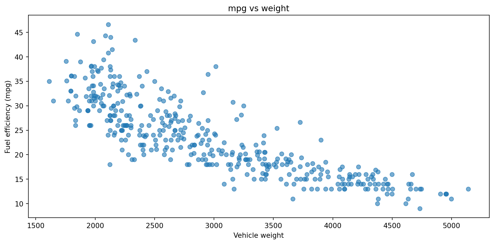
Dataset: car fuel efficiency dataset (mpg).
Better mpg → lower fuel consumption → lower emissions.
Intercept: 46.216524549017564
Slope : -0.007647342535779576
plt.scatter(mpg["weight"], mpg["mpg"], alpha=0.6, label="Observed")
order = np.argsort(mpg["weight"].values)
plt.plot(mpg["weight"].values[order], mpg["pred_mpg"].values[order], label="OLS fit")
plt.xlabel("Vehicle weight")
plt.ylabel("Fuel efficiency (mpg)")
plt.title("mpg vs weight (OLS fit)")
plt.legend()
plt.tight_layout()
plt.show()
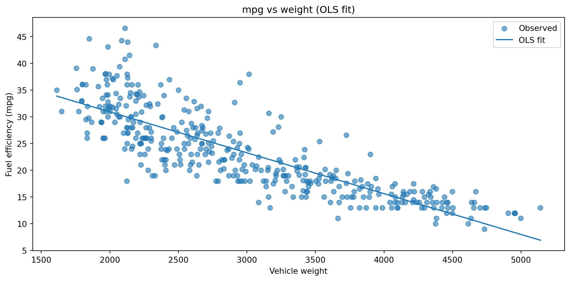
This looks somewhat reasonable… but is it good enough?

Watch for:

Warning
If we see:
then a simple straight line may be too naïve for some ranges.

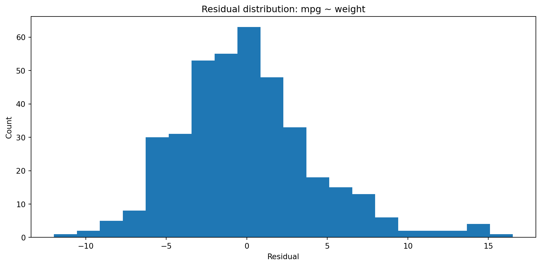
Warning
Again: we’re looking for rough symmetry and no wild tails.
But remember:
Even a nice residual histogram doesn’t fix a systematically wrong relationship.
Two common misuses in high-impact settings:
Non-linear relationship forced into a line
Wrong data type / units in serious decisions
When this happens:
From earlier ML modules (M38), for regression we often use:
Example (mpg):
MAE : 3.2787024115118464
RMSE: 4.321645126270701
R^2 : 0.6926304331206254
Warning
But remember:
Good metrics do not fix broken assumptions or bad causal reasoning.
fig, axes = plt.subplots(2, 2, figsize=(10, 8))
# 1. Data + fit
axes[0, 0].scatter(mpg["weight"], mpg["mpg"], alpha=0.6)
order = np.argsort(mpg["weight"].values)
axes[0, 0].plot(mpg["weight"].values[order], mpg["pred_mpg"].values[order])
axes[0, 0].set_xlabel("Weight")
axes[0, 0].set_ylabel("mpg")
axes[0, 0].set_title("mpg vs weight (fit)")
# 2. Residuals vs fitted
axes[0, 1].scatter(mpg["pred_mpg"], mpg["resid_mpg"], alpha=0.6)
axes[0, 1].axhline(0, linestyle="--")
axes[0, 1].set_xlabel("Fitted mpg")
axes[0, 1].set_ylabel("Residual")
axes[0, 1].set_title("Residuals vs fitted")
# 3. Residuals vs weight
axes[1, 0].scatter(mpg["weight"], mpg["resid_mpg"], alpha=0.6)
axes[1, 0].axhline(0, linestyle="--")
axes[1, 0].set_xlabel("Weight")
axes[1, 0].set_ylabel("Residual")
axes[1, 0].set_title("Residuals vs weight")
# 4. Histogram
axes[1, 1].hist(mpg["resid_mpg"], bins=15)
axes[1, 1].set_xlabel("Residual")
axes[1, 1].set_ylabel("Count")
axes[1, 1].setTitle = ("Residual histogram")
plt.tight_layout()
plt.show()
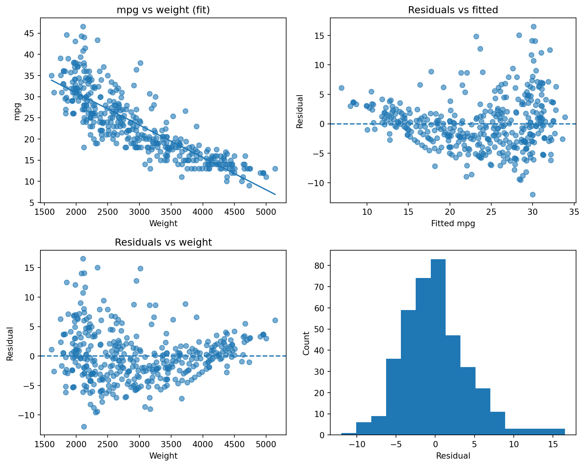
These four views give a compact visual check of OLS assumptions.

Before you brag about an \(R^2\) value (in any high-impact domain), ask:
These are lightweight but powerful habits.
OLS feels simple, but in high-impact domains:
Mitigations at this level:
Q1: Which statement best captures the geometric view of OLS?
A. OLS chooses coefficients so that the predictions equal the observed values exactly.
B. OLS finds the projection of \(y\) onto the column space of \(X\).
C. OLS chooses coefficients that minimize the absolute residuals.
D. OLS finds the largest possible R² on the test set.
Q: You fit a linear model for fuel efficiency and plot residuals vs fitted values. You see a clear U-shaped pattern.
1–2 sentences: what does this suggest, and what might you do?
Q3: Fill in the blanks: The OLS estimate \(\hat\beta\) satisfies the normal equations \[ \_\_\_\_\_\_\_\_ X\hat\beta = X^\top y. \]
Q4: You have two regression models for disease progression:
Which model is more appropriate, and why?