M38: What is Machine Learning?

CSCI 1109 — Practical Data Science

Frank Rudzicz

Machine learning

  • What do we actually mean by a machine learning model in this course?
  • How do ML tasks (classification, regression, etc.) fit into the broader data science pipeline you’ve already seen?
  • Why do we keep talking about train / validation / test splits, and what can go wrong if we ignore them?
  • How do simple ML workflows look in Python code (at the CSCI 1109 level)?

Learning outcomes

By the end of this module, you should be able to:

  1. Explain what machine learning is and how it differs from “just writing rules.”
  2. Classify common ML tasks as regression, classification, or other types (e.g., clustering).
  3. Describe and justify a basic train / validation / test split for supervised learning.
  4. Implement a simple ML workflow in Python that:
    • splits data;
    • trains a model;
    • evaluates it on held-out data.
  5. Diagnose basic evaluation mistakes, including overfitting and data leakage.

Conceptual scaffold

From rules to models: what is ML?

Traditional programming

  • You write explicit rules:
    if balance < 0 and days_overdue > 30: flag = "risky"
  • Data are inputs; program is fixed and brittle.

Machine learning (ML)

  • We provide examples of inputs and outputs.
    • Inputs: features (e.g., GPA, previous quizzes, activity logs).
    • Outputs: labels/targets (e.g., “completed quiz next week: yes/no”).
  • A learning algorithm searches for rules that work well on the examples.
  • After training, the model can make predictions on new cases.

Shortcut definition for this course

Machine learning is about learning patterns from data so we can make predictions or decisions about new cases, without hand-coding all the rules.

ML inside the data science lifecycle

You’ve already seen:

  • Question framing: what decision are we supporting?
  • Data cleaning & prep: missingness, duplicates, scaling, encoding.
  • Exploration & visualization: distributions, relationships, suspicious patterns.
  • Causal thinking: correlation vs causation; experiments vs observational designs.

Now we add:

  • Supervised ML: learn a mapping from features → target.
  • Evaluation: check how well the model generalizes to unseen data.

ML is not the whole story; it’s one tool in a bigger, messy data science pipeline.

Core ML task types (at our level)

Supervised learning

We have input features \(X\) and a target \(y\) for each example.

  • Classification
    • Target: discrete categories (e.g., “at risk” vs “not at risk”).
    • Examples: fraud detection, email spam, disease prediction.
  • Regression
    • Target: numeric value (e.g., hours studied next week).
    • Examples: predicting tip percentage, house price, wait time.

Unsupervised learning

  • No explicit labels; we only have features \(X\).
    • Example: clustering customers into “engagement profiles”

In and out: \(\color{blue}{X}\) and \(\color{red}{y}\)

We’ll use this notation a lot:

  • \(\color{blue}{X}\) (capital): all your input data — a matrix of shape \((n, d)\)
    • \(n\) = number of examples (rows: students, patients, transactions, …)
    • \(d\) = number of features per example
  • \(\color{red}{y}\) (lowercase vector): the target(s) we care about — shape \((n,)\)

Think of one row of \(\color{blue}{X}\) as one data point.

Code
import pandas as pd

df = pd.DataFrame({
    "time_on_platform_hours": [1.2, 3.4, 5.1],
    "avg_quiz_score": [55, 78, 88],
    "will_subscribe": [0, 1, 1],
})

def color_xy_cols(col):
    if col.name in ["time_on_platform_hours", "avg_quiz_score"]:
        # X columns → light blue
        return ['background-color: #e6f2ff'] * len(col)
    elif col.name == "will_subscribe":
        # y column → light red
        return ['background-color: #ffe6e6'] * len(col)
    else:
        return [''] * len(col)

df.style.apply(color_xy_cols)
  time_on_platform_hours avg_quiz_score will_subscribe
0 1.200000 55 0
1 3.400000 78 1
2 5.100000 88 1
Code
X = df[["time_on_platform_hours", "avg_quiz_score"]].values
y = df["will_subscribe"].values

print("X shape:", X.shape)  # (n, d)
print("y shape:", y.shape)  # (n,)
X shape: (3, 2)
y shape: (3,)

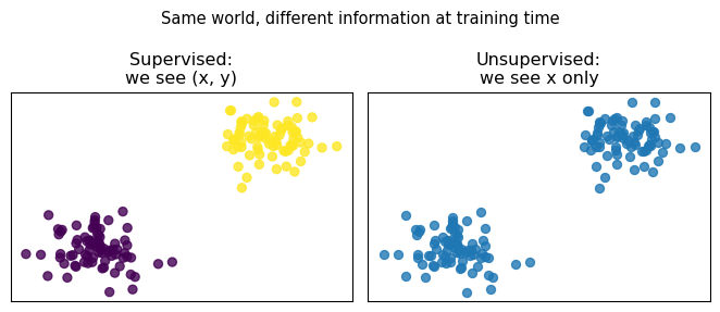
Supervised vs unsupervised

Code
import numpy as np
import matplotlib.pyplot as plt

rng = np.random.default_rng(3151)

n_per = 80
X1 = rng.normal([2, 2], 0.6, size=(n_per, 2))
X0 = rng.normal([-2, -2], 0.6, size=(n_per, 2))

X = np.vstack([X1, X0])
y = np.concatenate([np.ones(n_per), np.zeros(n_per)])

fig, axes = plt.subplots(1, 2, figsize=(7, 3))

axes[0].scatter(X[:, 0], X[:, 1], c=y, alpha=0.8)
axes[0].set_title("Supervised:\nwe see (x, y)")
axes[0].set_xticks([]); axes[0].set_yticks([])

axes[1].scatter(X[:, 0], X[:, 1], alpha=0.8)
axes[1].set_title("Unsupervised:\nwe see x only")
axes[1].set_xticks([]); axes[1].set_yticks([])

fig.suptitle("Same world, different information at training time", fontsize=11)
fig.tight_layout()
plt.show()

  • Supervised: the learner is told which points are, e.g., “positive” vs “negative”.
  • Unsupervised: the learner only sees the cloud of \(x\)’s and must discover structure without labels.

Unifying idea: learning from data

We’ll use a simple notation:

  • Input features: \(\color{blue}{x \in \mathcal{X}}\) (e.g., images, tabular records, text).
  • Targets / labels: \(\color{red}{y \in \mathcal{Y}}\) (e.g., classes, real numbers, next token).
  • Data come from an unknown distribution \((\color{blue}{X},\color{red}{Y}) \sim p(\color{blue}{x},\color{red}{y})\).

🚨 Machine learning (for this course):

Learn a function \(f_\theta : \mathcal{X} \to \mathcal{Y}\) that performs well on new samples from the same (or similar) distribution.

A probability surface over \(\color{blue}{(x_1, x_2)}\)

Code
import numpy as np
import pandas as pd
from sklearn.linear_model import LogisticRegression
import plotly.graph_objects as go

# Synthetic 2D data, similar to our earlier example
rng = np.random.default_rng(3151)
n_pos, n_neg = 80, 80

time_pos = rng.normal(5.0, 1.0, size=n_pos)
quiz_pos = rng.normal(80.0, 5.0, size=n_pos)

time_neg = rng.normal(1.5, 0.7, size=n_neg)
quiz_neg = rng.normal(55.0, 7.0, size=n_neg)

X = np.vstack([
    np.column_stack([time_pos, quiz_pos]),
    np.column_stack([time_neg, quiz_neg]),
])
y = np.concatenate([
    np.ones(n_pos, dtype=int),
    np.zeros(n_neg, dtype=int),
])

df = pd.DataFrame({
    "time_on_platform_hours": X[:, 0],
    "avg_quiz_score": X[:, 1],
    "will_subscribe": y,
})

# Fit logistic regression
log_reg = LogisticRegression()
log_reg.fit(X, y)

# Grid over feature space
x1_grid = np.linspace(df["time_on_platform_hours"].min()-1,
                      df["time_on_platform_hours"].max()+1, 60)
x2_grid = np.linspace(df["avg_quiz_score"].min()-5,
                      df["avg_quiz_score"].max()+5, 60)
xx, yy = np.meshgrid(x1_grid, x2_grid)
grid = np.c_[xx.ravel(), yy.ravel()]

probs = log_reg.predict_proba(grid)[:, 1].reshape(xx.shape)

# Build interactive 3D surface + points
surface = go.Surface(
    x=xx,
    y=yy,
    z=probs,
    colorscale="Viridis",
    showscale=False,
    opacity=0.8,
)

points = go.Scatter3d(
    x=df["time_on_platform_hours"],
    y=df["avg_quiz_score"],
    z=df["will_subscribe"],
    mode="markers",
    marker=dict(
        size=4,
        color=df["will_subscribe"],
        colorscale="Viridis",
        opacity=0.9,
    ),
    name="data",
)

fig = go.Figure(data=[surface, points])
fig.update_layout(
    scene=dict(
        xaxis_title="time_on_platform_hours",
        yaxis_title="avg_quiz_score",
        zaxis_title="P(will_subscribe=1)",
    ),
    margin=dict(l=0, r=0, b=0, t=30),
    title="Probability surface over $(x_1, x_2)$",
)

fig
  • The horizontal axes are features (here, two dimensions of \(\color{blue}{x}\)).
  • The height is the model’s estimate of \(P(\color{red}{y=1} \mid \color{blue}{x})\).
  • Supervised learning in this course is mostly about learning functions like this that generalize to new \(\color{blue}{(x_1, x_2)}\).

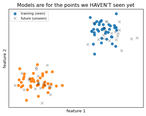
Why we care about models

In every learning setting, the game is:

Use data we do have (training) to build a model that performs well on data we haven’t seen yet (future samples from the same process).

Code
import numpy as np
import matplotlib.pyplot as plt

rng = np.random.default_rng(3151)

# Training data (what we see)
n_train = 80
X_train_pos = rng.normal([2, 2], 0.6, size=(n_train // 2, 2))
X_train_neg = rng.normal([-2, -2], 0.6, size=(n_train // 2, 2))

# "Future" data (what the model will actually face)
n_future = 40
X_future = np.vstack([
    rng.normal([2, 2], 0.6, size=(n_future // 2, 2)),
    rng.normal([-2, -2], 0.6, size=(n_future // 2, 2)),
])

fig, ax = plt.subplots(figsize=(5, 4))

# Training points
ax.scatter(X_train_pos[:, 0], X_train_pos[:, 1],
           label="training (seen)", alpha=0.9)
ax.scatter(X_train_neg[:, 0], X_train_neg[:, 1],
           alpha=0.9)

# Future points
ax.scatter(X_future[:, 0], X_future[:, 1],
           label="future (unseen)", alpha=0.3,
           marker="x", linewidths=1.5, color="black")

ax.set_xticks([]); ax.set_yticks([])
ax.set_xlabel("feature 1")
ax.set_ylabel("feature 2")
ax.set_title("Models are for the points we HAVEN'T seen yet")
ax.legend(loc="upper left", fontsize=8)

plt.tight_layout()
plt.show()

Tip

Every metric we compute on a test set is trying to estimate:

“How will this model behave on future data from this process?”

If we’re only winning on the points we’ve already seen, we’re not doing machine learning — we’re doing memorization.

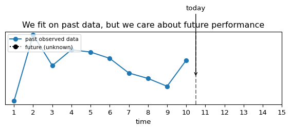
Today’s data, tomorrow’s decisions

Think of every ML project as a small time-travel experiment:

  • Today: we have a dataset \(\{(\color{blue}{x_i}, \color{red}{y_i})\}_{i=1}^n\) from the past.
  • Tomorrow: we’ll see new \(\color{blue}{X^*}\) and have to make decisions before we know \(\color{red}{Y^*}\).

We often (not always) want a model \(f_\theta\) to help with tomorrow’s decisions, not just to explain yesterday.

Train / validation / test: definitions

  • Train set
    • Used to fit the model parameters.
    • The model is allowed to see this many times.
  • Validation (val) set
    • Used to choose design decisions:
      • Hyperparameters (e.g., value of \(k\) in k-NN).
      • Which features to include/exclude.
      • Which model family to pick.
    • We compare alternatives on the val set, not the test set.
  • Test set
    • Used once at the end for final performance.
    • We do not touch it during model design.
    • We report test performance in our write-up.

Doing the splits

-Think of the workflow as a conveyor belt:

  • Split into three partitions. By convention”
    1. ~60–70%: Train.
    2. ~15–20%: Validation.
    3. ~15–20%: Test.
  • Feedback loop:
    • Train → Validate → tweak → Train …
    • Only when satisfied: Train+Val → Test.
Code
%%{init: {
  "theme": "neutral",
  "fontsize": "12px",
  "flowchart": { "curve": "basis" }
}}%%
flowchart TD

classDef bigNode   fill:#ffffff,stroke:#333,stroke-width:1.5px,font-size:18px,padding:18px;
classDef smallNode fill:#ffffff,stroke:#333,stroke-width:1.5px,font-size:12px,padding:8px;
classDef noteNode  fill:#ffffff,stroke-dasharray:3 3,stroke:#555,font-size:12px;

subgraph Splits[ ]
  direction TB
  T["TRAIN (~60–70%<br>of data)"]:::bigNode
  V["VALIDATION<br>(~15–20%)"]:::smallNode
  Te["TEST<br>(~15–20%)"]:::smallNode
end

T  -->|train models| V
V  -->|tune &<br>try again| T
V  -->|final chosen<br> model| Te

Note["[Note] Never tune on TEST"]:::noteNode
Te -.-> Note

%%{init: {
  "theme": "neutral",
  "fontsize": "12px",
  "flowchart": { "curve": "basis" }
}}%%
flowchart TD

classDef bigNode   fill:#ffffff,stroke:#333,stroke-width:1.5px,font-size:18px,padding:18px;
classDef smallNode fill:#ffffff,stroke:#333,stroke-width:1.5px,font-size:12px,padding:8px;
classDef noteNode  fill:#ffffff,stroke-dasharray:3 3,stroke:#555,font-size:12px;

subgraph Splits[ ]
  direction TB
  T["TRAIN (~60–70%<br>of data)"]:::bigNode
  V["VALIDATION<br>(~15–20%)"]:::smallNode
  Te["TEST<br>(~15–20%)"]:::smallNode
end

T  -->|train models| V
V  -->|tune &<br>try again| T
V  -->|final chosen<br> model| Te

Note["[Note] Never tune on TEST"]:::noteNode
Te -.-> Note

🔑 Key ideas:

  • Splits are about honest performance on data the model has never seen.
  • We want to avoid “peeking” at the test set while we design the model.

❌ Anti-example: Train == test

A common (and bad) pattern:

  1. Load entire dataset.
  2. Train model on all rows.
  3. Report accuracy evaluated on the same data.

Why this is wrong:

  • The model can memorize weird quirks of the specific sample (overfitting).
  • Reported performance is “too good to be true.”
  • When deployed to new data, performance often crashes.

If your model has never been checked on truly unseen data, you have no idea how it will behave in the real world.

Error & generalization

  • Data: examples \((x_i, y_i)\) for \(i = 1, \dots, n\).
  • Model: \(f_\theta(x)\) with parameters \(\theta\) learned from data.
  • Loss function \(\ell(f_\theta(x), y)\):
    • Classification example: 0/1 loss (1 if wrong, 0 if correct).
    • Regression example: squared error \((f_\theta(x) - y)^2\).

Empirical training loss (average error on train set):

\[ \hat{R}_{\text{train}}(\theta) = \frac{1}{n_{\text{train}}} \sum_{i \in \text{train}} \ell(f_\theta(x_i), y_i). \]

Validation loss is computed similarly, but over the validation set:

\[ \hat{R}_{\text{val}}(\theta) = \frac{1}{n_{\text{val}}} \sum_{i \in \text{val}} \ell(f_\theta(x_i), y_i). \]

  • We choose \(\theta\) (or hyperparameters) that keep validation error small.
  • The test error is our best guess at how the model will perform on new, real-world data.

Worked example 1

Classification with a simple split

🥅 Goal: predict whether a household’s daily water use will exceed a local conservation target (e.g., 150 liters per person per day).

Why this might matter:

  • City planners want to identify high-usage days so they can plan infrastructure and conservation campaigns.
  • Households might opt in to receive reminders or tips when they are likely to exceed the target.
  • The focus is on supporting sustainable resource use, not blaming individual households.

Assume we have a small synthetic dataset with:

  • temp_c – average outdoor temperature that day (°C),
  • household_size – number of people in the household,
  • has_garden – 1 if the household has a garden/lawn, 0 otherwise,
  • is_weekend – 1 if the day is Saturday/Sunday, 0 otherwise,
  • above_target – 1 if daily water use exceeded the conservation threshold, 0 otherwise.
Code
import numpy as np
import pandas as pd

rng = np.random.default_rng(1109)
n = 128

temp_c = rng.integers(10, 35, size=n)          # cooler to very warm days
household_size = rng.integers(1, 6, size=n)    # 1–5 people
has_garden = rng.integers(0, 2, size=n)        # 0 or 1
is_weekend = rng.integers(0, 2, size=n)        # 0 or 1

# A simple rule-of-thumb model for daily water (liters), plus noise
daily_liters = (
    (80 + 20 * household_size) +
    3 * (temp_c - 20) +          # hotter days → more use
    25 * has_garden +
    15 * is_weekend +
    rng.normal(0, 15, size=n)    # random noise (float)
)

target_liters = 150
above_target = (daily_liters > target_liters).astype(int)

df = pd.DataFrame({
    "temp_c": temp_c,
    "household_size": household_size,
    "has_garden": has_garden,
    "is_weekend": is_weekend,
    "above_target": above_target,
})

df.head()
temp_c household_size has_garden is_weekend above_target
0 24 4 1 0 1
1 20 4 0 1 1
2 30 1 0 1 0
3 15 4 1 0 1
4 27 1 0 0 0

Train/validation/test split in code

We’ll create an ~60% / 20% / 20% split and keep class balance using stratified splits (our dataset is large enough for that here).

Code
from sklearn.model_selection import train_test_split

features = ["temp_c", "household_size", "has_garden", "is_weekend"]
target = "above_target"

X = df[features]
y = df[target]

# First: train_temp vs test (stratify to preserve 0/1 proportions)
X_train, X_temp, y_train, y_temp = train_test_split(
    X,
    y,
    test_size=0.2,
    random_state=1109,
    stratify=y,
)

# Second: val vs test from the temporary set (also stratified)
X_val, X_test, y_val, y_test = train_test_split(
    X_temp,
    y_temp,
    test_size=0.5,
    random_state=1109,
    stratify=y_temp,
)

len(X_train), len(X_val), len(X_test)
(102, 13, 13)
  • We use stratify=y to keep class proportions balanced in each split.
    • With 128 rows and reasonably balanced classes, each split still has at least a few examples of both 0 and 1, so stratification is safe.
  • On very tiny datasets, stratifying multiple times can fail; on realistic tabular data, this pattern is common.

Fit & evaluate k-NN

Code
from sklearn.neighbors import KNeighborsClassifier
from sklearn.metrics import accuracy_score

knn = KNeighborsClassifier(n_neighbors=3)

# Train the model
knn.fit(X_train, y_train)

# Evaluate on train, val, and test
y_train_pred = knn.predict(X_train)
y_val_pred   = knn.predict(X_val)
y_test_pred  = knn.predict(X_test)

acc_train = accuracy_score(y_train, y_train_pred)
acc_val   = accuracy_score(y_val, y_val_pred)
acc_test  = accuracy_score(y_test, y_test_pred)

print("Train accuracy:", acc_train)
print("Val accuracy:  ", acc_val)
print("Test accuracy: ", acc_test)
Train accuracy: 0.9019607843137255
Val accuracy:   0.9230769230769231
Test accuracy:  0.8461538461538461

✏️ Think

  • If train accuracy ≫ val/test accuracy, what might that suggest about overfitting to this particular sample of households?
  • If val accuracy is higher for k=5 than k=3, which should we prefer (and why)?
  • What other features might improve this model (e.g., building type, recent rainfall), and how might we accidentally introduce data leakage if we’re not careful about which information is available at prediction time?

Design choices & subtle pitfalls

Key design decisions even in this tiny example:

  • Random state & reproducibility
    • Setting random_state helps you and your future self reproduce results.
  • Stratified splits
    • For classification, use stratify=y so each split has similar class balances.
  • Feature scaling
    • For distance-based models (like k-NN), differing feature scales matter.
    • In practice, we’d use a Pipeline with StandardScaler before k-NN.
  • Data leakage
    • Don’t compute features using future information.
    • Don’t fit scalers or imputers on the whole dataset; fit them inside a pipeline using only the training data.

Worked example 2

Regression on a familiar dataset

Let’s predict tip percentage from the tips dataset (you used it earlier).

Goal: model tip_pct = tip / total_bill from features like:

  • total_bill
  • size (party size)
  • smoker (encoded)
  • time (lunch/dinner, encoded)
Code
import seaborn as sns
from sklearn.model_selection import train_test_split
from sklearn.linear_model import LinearRegression
from sklearn.metrics import mean_absolute_error

tips = sns.load_dataset("tips").dropna().copy()
tips["tip_pct"] = tips["tip"] / tips["total_bill"]

tips.head()
total_bill tip sex smoker day time size tip_pct
0 16.99 1.01 Female No Sun Dinner 2 0.059447
1 10.34 1.66 Male No Sun Dinner 3 0.160542
2 21.01 3.50 Male No Sun Dinner 3 0.166587
3 23.68 3.31 Male No Sun Dinner 2 0.139780
4 24.59 3.61 Female No Sun Dinner 4 0.146808

Encoding + split + regression

Code
# Simple feature set: numeric + one-hot-encoded categorical
df = tips[["total_bill", "size", "sex", "smoker", "time", "tip_pct"]]

df_enc = pd.get_dummies(
    df,
    columns=["sex", "smoker", "time"],
    drop_first=True
)

X = df_enc.drop(columns=["tip_pct"])
y = df_enc["tip_pct"]

X_train, X_test, y_train, y_test = train_test_split(
    X, y, test_size=0.2, random_state=1109
)

linreg = LinearRegression()
linreg.fit(X_train, y_train)

y_train_pred = linreg.predict(X_train)
y_test_pred = linreg.predict(X_test)

mae_train = mean_absolute_error(y_train, y_train_pred)
mae_test = mean_absolute_error(y_test, y_test_pred)

print("Train MAE:", mae_train)
print("Test MAE: ", mae_test)
Train MAE: 0.03772670011766519
Test MAE:  0.044119962713874486
  • We use MAE (mean absolute error) since it’s in the same units as tip_pct.
  • Discussion: is this error “big” in context?

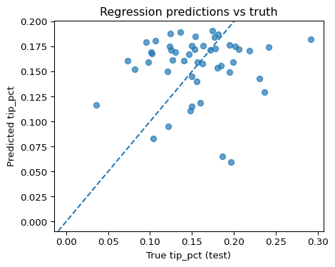
Visualizing predictions vs reality

Even simple plotting helps diagnose problems:

Code
import matplotlib.pyplot as plt

plt.figure(figsize=(5, 4))
plt.scatter(y_test, y_test_pred, alpha=0.7)
plt.xlabel("True tip_pct (test)")
plt.ylabel("Predicted tip_pct")
plt.title("Regression predictions vs truth")
plt.axline((0, 0), slope=1, linestyle="--")  # ideal line
plt.tight_layout()
plt.show()

✏️ Think

  • Are points roughly clustered around the diagonal, or is there systematic bias?
  • Are errors larger for certain ranges (e.g., very high tip_pct)?
  • How might missing features (e.g., service quality) limit performance?

Summary

Evaluation metrics & decision context

Even in these tiny examples, metrics must match decisions:

  • Classification
    • Accuracy is OK when classes are balanced and mistakes are equally costly.
    • In imbalanced or high-stakes settings, we’ll care about other metrics
  • Regression
    • MAE vs RMSE:
      • MAE: robust, interpretable in original units.
      • RMSE: \[ \text{RMSE} = \sqrt{ \frac{1}{n_{\text{test}}} \sum_{i=1}^{n_{\text{test}}} \bigl(y_i - \hat{y}_i\bigr)^2 } \]
      punishes large errors more; can be useful when big mistakes are very bad.
  • In practice
    • Always ask: “What is this model for? Which mistakes hurt most?”
    • Tie your metric choices to the stakeholder scenario.

❌ Anti-example: data leakage in splitting

Imagine we’re predicting whether a student passes the final exam:

  • Features include:
    • midterm_mark
    • assignment_average
    • final_mark 👈 (this is the label itself!)

🤪 Suppose we accidentally:

  1. Use final_mark to compute a feature like overall_course_average, then
  2. Predict “pass_final” using that feature.

🤷 What went wrong?

  • The model has direct access to the thing we want to predict (or something computed with it).
  • Train and test performance will look amazing.
  • In reality, the model is useless before the final exam happens.

Rule of thumb: your features should use only information available at prediction time.

Ethics & risks in ML evaluation

Even in “toy” educational examples, evaluation choices matter:

  • Biased splits
    • If the train set under-represents certain groups (e.g., part-time students), the model may perform poorly for them.
    • Time-based splits matter: training on old cohorts may not generalize to newer ones.
  • Hiding uncertainty
    • Reporting a single accuracy number without context hides variance.
    • Use confidence intervals, replicate splits, and clear caveats where possible.
  • Misuse of models
    • Using a soft educational risk model to make hard decisions (e.g., remove students from a program) without human oversight can be harmful.
    • Share limitations and failure modes in your write-ups (this is part of responsible data science).

Mitigations (at 1109 level):

  • Stratified splits; fairness checks by subgroup.
  • Clear documentation of data sources, time windows, and what the model can/cannot do.
  • In assignments, explicit prompts to reflect on limitations.

Quick checks

  1. Which of the following is a classification problem?

    A. Predicting tomorrow’s temperature in °C.
    B. Predicting whether a transaction is fraudulent (yes/no).
    C. Predicting the number of minutes a student will study.
    D. Predicting the total number of visitors next week.

  2. Why do we keep a separate test set?

    A. To have more data to train on.
    B. To tune hyperparameters like k in k-NN.
    C. To get an unbiased estimate of performance on new data.
    D. To debug code more easily.

  3. You train a model and see:

    • Train accuracy: 0.99
    • Validation accuracy: 0.78
    • Test accuracy: 0.77

    Which is the most likely explanation?

    A. The model is underfitting.
    B. The model is overfitting the training data.
    C. The dataset is too large.
    D. The train/val/test split is impossible.

  4. Which situation is an example of data leakage?

    A. Using only 80% of the data for training.
    B. Fitting a scaler (mean/variance) on the full dataset before splitting.
    C. Using a random seed in train_test_split.
    D. Stratifying the split by class label.