M23 - Sampling & bootstrapping in Python

CSCI 1109 — Practical Data Science

Frank Rudzicz

Why sampling & bootstrapping?

Motivating story (hospital wait times)

A hospital reports:

“Average emergency wait time last week was 42 minutes.”
Real questions decision-makers care about:
- How much could that number have changed if different patients showed up?
- Is this week clearly worse than last week?
- Are policy changes helping or just noise?

Goal of this module

Build simulation and resampling tools in Python to:
- Reason about sampling variation
- Construct interval estimates (e.g., “42 minutes, plus/minus a bit”)
- Prepare for later modules on p-values & hypothesis tests

Code

import numpy as np
import pandas as pd
import matplotlib.pyplot as plt

# For reproducibility
rng = np.random.default_rng(1109)

# Make plots a bit larger by default
plt.rcParams["figure.figsize"] = (6, 4)
plt.rcParams["axes.grid"] = True

Learning outcomes

After this module, you should be able to…

Explain the difference between a population, a sample, and a sampling distribution.
Simulate sampling variation for simple statistics (means, proportions) using Python.
Implement a basic bootstrap procedure (for a mean and a difference in proportions).
Construct and interpret a bootstrap confidence interval in a decision context.
Diagnose when bootstrap-style methods are reasonable, and when sampling bias breaks everything.

Conceptual scaffold

Populations, samples, and statistics

Key concepts

Population: the full set of units you care about
e.g., all ER visits this year.
Sample: the subset you actually observe
e.g., 120 visits from last week.
Statistic: a number computed from the sample
e.g., sample mean wait time, sample proportion of patients seen within 30 minutes.

Note

The sampling distribution of a statistic is the distribution you’d see if you could repeat your entire sampling process many times.

Why do we care about sampling distributions?

They let us answer questions like:

“If the true average wait time were 40 minutes, how extreme is our observed 48 minutes?”
“Is a difference of 3 percentage points in click-through rate actually meaningful, or just noise?”
“How wide should our ‘plus/minus’ interval be around a point estimate?”

Without some model of sampling variation, statements like

“The average is 42 minutes”

are incomplete. We need something like:

“Average is 42 minutes, and typical sampling variation is around ±5 minutes.”

Bootstrap: idea in one picture

Instead of:

Repeatedly sampling new data from the population (impossible in practice),

we:

Repeatedly resample with replacement from our existing sample.

This is our simulation-based stand-in for the true sampling distribution.

❌ Anti-example: treating one sample as “truth”

A manager says:
“We measured 50 patients. The average wait was 37.6 minutes.
Therefore, from now on, we’ll just say the true average is 37.6.”

Issues:

Ignores randomness in who showed up that day.
Ignores small sample size (50).
Ignores selection bias: maybe that day had a staffing issue, or a snowstorm.

🙅🏽 Takeaway anti-pattern

Using a single sample statistic as a precise truth claim instead of as an estimate with uncertainty.

Bootstrap & sampling simulations help us visualize and quantify that uncertainty.

Math lens

Notation: sample mean & its variability

Let

\(X_1, \dots, X_n\) = wait times for \(n\) patients.
Sample mean:

\[ \bar{X} = \frac{1}{n}\sum_{i=1}^n X_i \]

In theory (under some assumptions):

The sampling distribution of \(\bar{X}\) is centered at the true mean \(\mu\).
Its spread (standard error) shrinks like \(1/\sqrt{n}\).

But:

We often don’t know the population distribution.
Deriving formulas for every new statistic is unrealistic

Bootstrap idea: approximate the sampling distribution of \(\bar{X}\) by resampling our data.

For a more formal treatment of the probability and statistics ideas behind this, see Deisenroth, Faisal, and Ong (2020).

Algorithm: bootstrap for a mean

Given a sample \(x_1, \dots, x_n\):

Compute the original statistic:

\[ \hat{\theta} = \bar{x} = \frac{1}{n}\sum_{i=1}^n x_i. \]
For \(b = 1, \dots, B\) (e.g., \(B = 2000\)):
1. Draw a bootstrap sample of size \(n\) with replacement from \(\{x_1,\dots,x_n\}\).
2. Compute the statistic on this sample: \(\hat{\theta}^{(b)}\).
Use the collection \(\{\hat{\theta}^{(1)}, \dots, \hat{\theta}^{(B)}\}\) to:
- Estimate the standard error: sample std of \(\hat{\theta}^{(b)}\).
- Build confidence intervals using percentiles (e.g., 2.5th and 97.5th).

This same pattern works for lots of statistics: medians, proportions, differences, etc.

🔬 Deeper technical detail (optional)

The bootstrap works best when:

Observations are independent and identically distributed (i.i.d.).
The statistic is a “smooth” function of the distribution.

If these conditions hold (roughly):

The bootstrap distribution converges to the true sampling distribution as:
- Sample size \(n\) grows
- Number of bootstrap resamples \(B\) grows

In more advanced courses, you’ll see:

Rate-of-convergence results (e.g., \(n \to \infty\))
Variants like the parametric bootstrap and block bootstrap (for dependent data)

For this course, we treat the bootstrap as a practical simulation tool
and focus on when it’s appropriate and how to interpret it.

For a deeper, classic treatment of bootstrap theory and practice, see Efron and Tibshirani (1994).

Worked example 1

Example 1: synthetic ER wait-time data

We’ll simulate data for 120 ER visits. Two triage levels:

"urgent": typically shorter waits
"non-urgent": typically longer waits

Code

n = 120

triage = rng.choice(["urgent", "non-urgent"], size=n, p=[0.4, 0.6])

wait_times = np.where(
    triage == "urgent",
    rng.normal(loc=30, scale=8, size=n),   # urgent: shorter waits
    rng.normal(loc=50, scale=10, size=n)   # non-urgent: longer waits
)

# Ensure no negative or crazy-small times
wait_times = np.clip(wait_times, 5, None)

er = pd.DataFrame({"triage": triage, "wait_min": wait_times})
er.head()

	triage	wait_min
0	urgent	28.277796
1	urgent	37.777020
2	urgent	41.910784
3	urgent	20.331177
4	non-urgent	35.585020

Inspecting the sample

Code

er.describe(include="all")

	triage	wait_min
count	120	120.000000
unique	2	NaN
top	non-urgent	NaN
freq	67	NaN
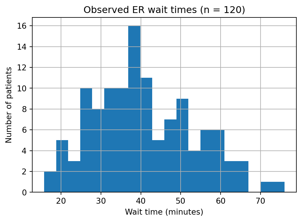
mean	NaN	40.769709
std	NaN	12.752208
min	NaN	15.771329
25%	NaN	31.257241
50%	NaN	39.099323
75%	NaN	49.376112
max	NaN	76.009549

✏️ What do you notice about:
- Typical wait times (mean, median)?
- The spread (std, min/max)?
- Count of observations?

Quick visualization:

Code

ax = er["wait_min"].hist(bins=20)
ax.set_xlabel("Wait time (minutes)")
ax.set_ylabel("Number of patients")
ax.set_title("Observed ER wait times (n = 120)");

Bootstrap: mean wait time

We want a 95% bootstrap confidence interval for the mean wait time.

Code

n_boot = 2000
boot_means = []

for _ in range(n_boot):
    sample = er["wait_min"].sample(
        frac=1.0,
        replace=True,
        random_state=rng.integers(0, 1_000_000)
    )
    boot_means.append(sample.mean())

boot_means = np.array(boot_means)

orig_mean = er["wait_min"].mean()
ci_low, ci_high = np.percentile(boot_means, [2.5, 97.5])

orig_mean, (ci_low, ci_high)

(40.76970860065877, (38.508473145919304, 43.01662206678892))

First number = sample mean (point estimate)
Interval = bootstrap percentile 95% CI

Visualizing the bootstrap distribution

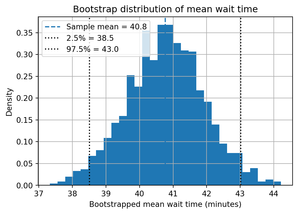
Interpretation:

Our best guess for the average wait time is ≈ orig_mean minutes.
A plausible range, given sampling variation, is about [ci_low, ci_high] minutes.
If the hospital claims “we keep average waits under 35 minutes,” does this look defensible?

Decision: is performance acceptable?

Suppose:

Policy target: average wait time ≤ 40 minutes.
Our bootstrap CI is \([L, U]\).

Cases:

If \(U < 40\): strong evidence we’re meeting the target.
If \(L > 40\): strong evidence we’re not meeting the target.
If CI overlaps 40: ambiguous → we need:
- More data (larger sample), or
- Different targets / metrics (e.g., 90th percentile wait, not mean).

The bootstrap doesn’t magically “prove” anything;
it quantifies uncertainty so we can make better decisions.

Worked example 2

Example 2: website signup experiment

Scenario:

We work at a company on the website team
Old landing page vs. new landing page.
Outcome = converted (1 if user signed up; 0 otherwise).

Simulated data:

Code

n_old, n_new = 200, 200

conv_old = rng.binomial(1, 0.08, size=n_old)  # 8% conversion
conv_new = rng.binomial(1, 0.11, size=n_new)  # 11% conversion

ab = pd.DataFrame({
    "variant": ["old"] * n_old + ["new"] * n_new,
    "converted": np.concatenate([conv_old, conv_new])
})

ab.head()

	variant	converted
0	old	0
1	old	0
2	old	0
3	old	0
4	old	0

Observed conversion rates

Code

ab_grouped = ab.groupby("variant")["converted"].agg(["mean", "sum", "count"])
ab_grouped

	mean	sum	count
variant
new	0.13	26	200
old	0.09	18	200

Let:

\(\hat{p}_\text{old}\) = conversion rate for old page
\(\hat{p}_\text{new}\) = conversion rate for new page
\(\hat{\delta} = \hat{p}_\text{new} - \hat{p}_\text{old}\) = observed difference

Code

p_old = ab_grouped.loc["old", "mean"]
p_new = ab_grouped.loc["new", "mean"]
delta_obs = p_new - p_old
delta_obs

0.04000000000000001

Question: Is this difference plausibly just noise, or real?

Bootstrap for difference in proportions

We’ll treat each bootstrap sample as:

Resample rows within the combined dataset with replacement.
Recompute conversion rates and their difference.

Code

n_boot = 4000
boot_diffs = []

for _ in range(n_boot):
    sample = ab.sample(
        frac=1.0,
        replace=True,
        random_state=rng.integers(0, 1_000_000)
    )
    mean_old = sample.loc[sample["variant"] == "old", "converted"].mean()
    mean_new = sample.loc[sample["variant"] == "new", "converted"].mean()
    boot_diffs.append(mean_new - mean_old)

boot_diffs = np.array(boot_diffs)

ci_low, ci_high = np.percentile(boot_diffs, [2.5, 97.5])
delta_obs, (ci_low, ci_high)

(0.04000000000000001, (-0.023277309956720487, 0.10006241450669022))

Visualizing the bootstrap difference

Code

ax = plt.hist(boot_diffs, bins=40, density=True)
plt.axvline(delta_obs, linestyle="--", label=f"Observed diff = {delta_obs:.3f}")
plt.axvline(ci_low, color="black", linestyle=":", label=f"2.5% = {ci_low:.3f}")
plt.axvline(ci_high, color="black", linestyle=":", label=f"97.5% = {ci_high:.3f}")
plt.axvline(0.0, color="red", linestyle="-.", label="No difference")

plt.xlabel("Bootstrapped difference in conversion (new - old)")
plt.ylabel("Density")
plt.title("Bootstrap distribution of conversion difference")
plt.legend();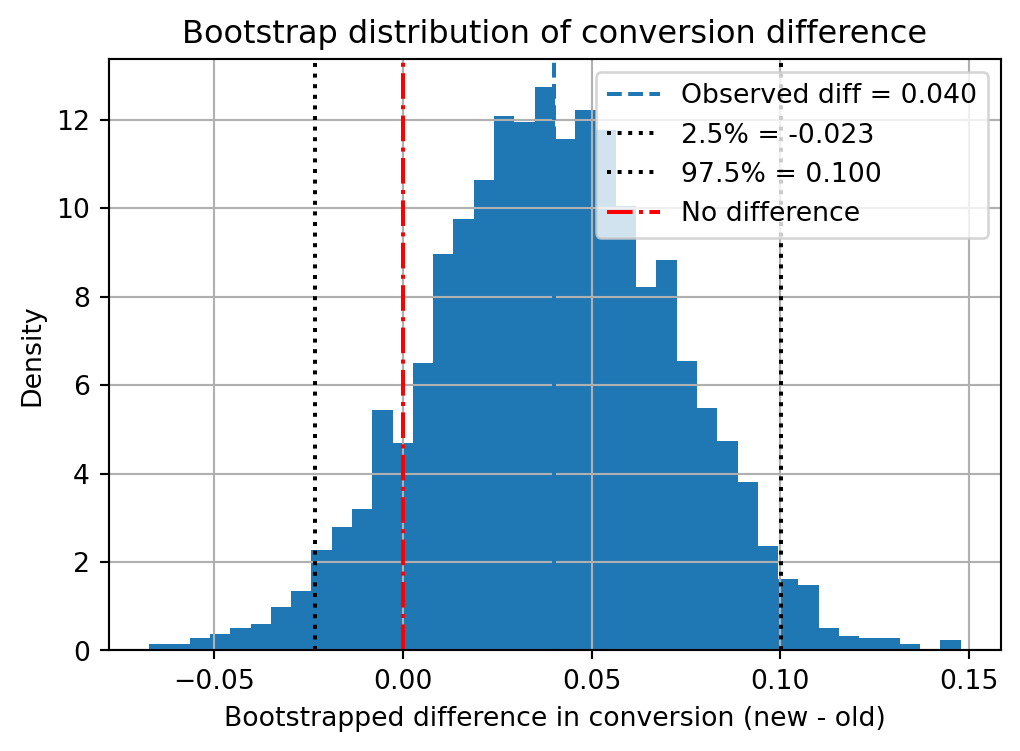

Interpretation:

If the CI barely crosses 0 → weak evidence of improvement.
If almost all bootstrap differences are > 0 → stronger evidence that new page is better.
BUT: this doesn’t address:
- Practical significance (is +2% worth the cost?)
- External validity (will this hold next month, on mobile, in other regions?)

Evaluation and quality checks

Before trusting a bootstrap-based conclusion, ask:

Sampling frame:
- Are users in the A/B test representative of future traffic?
Randomization:
- Were users truly randomly assigned to old vs new page?
Independence:
- Are observations approximately independent? (One user ≈ one row)
Stability:
- Does the effect persist if:
  - We change the bootstrap seed?
  - We slightly change the time window?

Diagnostics you can run:

Compare bootstrap CIs from different time slices.
Check if certain subgroups (e.g., mobile vs desktop) behave differently.
Use multiple metrics (e.g., click-through, downstream retention).

Wrapup

Bootstrapping in real Python libraries

SciPy
- 🔗 scipy.stats.bootstrap implements the generic bootstrap pattern you coded by hand.
- You pass in your data and a statistic function (e.g., np.mean), and it returns a bootstrap confidence interval.

from scipy.stats import bootstrap
import numpy as np

rng = np.random.default_rng(1109)
x = rng.normal(loc=75, scale=8, size=50)

# SciPy expects a tuple of arrays
res = bootstrap(
    (x,),
    np.mean,
    confidence_level=0.95,
    n_resamples=2000,
    method="percentile",
    random_state=rng,
)

res.confidence_interval.low, res.confidence_interval.high

scikit-learn
- Uses bootstrap-style resampling inside ensemble methods like:
  - BaggingClassifier, BaggingRegressor
  - RandomForestClassifier, RandomForestRegressor
- Also provides sklearn.utils.resample for general-purpose resampling:

from sklearn.utils import resample

# X, y could be any dataset (features, labels)
X_boot, y_boot = resample(X, y, replace=True, random_state=1109)

🔗 **Statsmodels (for later courses)**
- Some models can compute bootstrapped standard errors or CIs.
- Shows up more in advanced statistics and econometrics, but built on the same idea: resample, recompute, look at the distribution of the statistic.

Where could things go wrong?

Sampling bias:
- If your data over-represent certain groups (e.g., night-shift patients, high-income users), bootstrapping will faithfully reproduce that bias.
Data quality & privacy:
- Bootstrapping doesn’t “hide” individuals; repeated resampling may reveal rare cases.
- Be careful when sharing bootstrap samples or detailed logs.
Fairness & equity:
- “Average improvement” might mask harms to subgroups (e.g., longer waits for a particular demographic).
Overconfidence:
- Narrow CIs from non-representative or tiny samples are misleading.

Simple mitigations:

Inspect and compare key subgroups before and after changes.
Document how the sample was collected and who might be missing.
Combine bootstrap uncertainty with domain knowledge.

🔮 Bootstrapping and later topics

This module is an on-ramp to:

M32: Distributions, CLT intuition, p-values 😱
- Bootstrap gives a simulation-based view of sampling distributions.
- CLT provides an analytic view for some statistics.
Simulation-based hypothesis tests (later in the course)
- Randomization tests, permutation tests.
Machine learning
- Bagging and random forests resample data for model stability.
- Cross-validation uses repeated splits to estimate performance.

Real systems using resampling ideas

In practice, resampling-style ideas show up in:

Model validation:
- Repeated train/test splits, bootstrap aggregating.
Uncertainty estimation:
- Bootstrap CIs for complex models where formulas are messy.
Robustness checks:
- “What if we drop this subgroup?” or “What if we reweight these observations?”

Key mindset:

Rather than memorizing formulas, think:
“Can I simulate what would happen if I repeated this process many times?”

Quick check

Conceptual
You have a random sample of 200 patients’ blood pressures.
Which of the following is closest to the idea of a bootstrap distribution of the mean?

A. The distribution of the 200 observed blood pressures.
B. The distribution of means from many resamples with replacement of those 200 values.
C. The distribution of means from 200 new patients in the future.
D. The distribution of differences between two unrelated datasets.
Numeric (thought only)
You bootstrap the mean wait time and find a 95% CI of [38, 46] minutes.
Which statement is most reasonable?

A. There is a 95% chance the true mean is exactly 42 minutes.
B. With this sampling process, intervals built this way will cover the true mean about 95% of the time.
C. The true mean must be between 38 and 46 minutes, guaranteed.
D. At least 95% of future wait times will be between 38 and 46 minutes.
Design
Which situation breaks the basic bootstrap assumptions the most?

A. 500 independent product ratings from different customers.
B. 500 daily closing prices of one stock (strong time dependence).
C. 500 independent survey responses from randomly sampled voters.
D. 500 machine sensor readings, each from a different machine.
Interpreting a CI for a difference
In an A/B test, the bootstrap 95% CI for (new − old) conversion rate is [−0.01, 0.05].
Which is the best conclusion?

A. New page is definitely worse.
B. New page is definitely better.
C. Data are consistent with small harm, no change, or modest benefit; we need more data or other evidence.
D. New and old pages are identical in every way.

References

Deisenroth, Marc Peter, A. Aldo Faisal, and Cheng Soon Ong. 2020. Mathematics for Machine Learning. Cambridge: Cambridge University Press. https://mml-book.github.io/.

Efron, Bradley, and Robert J. Tibshirani. 1994. An Introduction to the Bootstrap. Monographs on Statistics and Applied Probability. New York: Chapman; Hall/CRC. https://cds.cern.ch/record/526679.