M19 - Vectors, matrices, broadcasting; linear ops

CSCI 1109 — Practical Data Science

Frank Rudzicz

Assumptions

  • By M19 you:
    • Have used Jupyter + Python for basic data analysis
    • Can load/inspect data with pandas and use .to_numpy()
    • Have seen simple train/test splits and baselines (e.g., predict the mean)
  • We won’t:
    • lean into formal linear algebra
    • Work with eigenvalues or matrix calculus
  • We will:
    • Treat NumPy arrays as vectors/matrices with shape

Outcomes

By the end of this module, you can:

  1. Represent a real situation as a vector with units.
  2. Use dot products to compute a score and explain it as a projection.
  3. Use a matrix to score many examples at once (vectorization).
  4. Predict and prevent broadcasting bugs by reasoning about shape.
  5. Communicate a claim with a baseline, a metric, and a severe test (train/test split).

Example: “Admissions as geometry”

The decision

A University committee wants a transparent first-pass scoring rule for applicants.

  • Who decides? Admissions committee.
  • What do they decide? Who to prioritize for review (not automated admission).
  • Why data science? To apply a rule consistently and check it against evidence.
  • Costs of errors:
    • False negative: miss a strong student (lost opportunity).
    • False positive: over-admit (resources stretched).

The data-generating process

Each applicant has measurements:

  • gpa (0–4 scale)
  • test_score (0–100)
  • extracurriculars (count)

We’ll generate a small dataset and keep the units explicit.

Intuition

  • A linear score is a weighted sum:

    • GPA matters a lot
    • test score matters some
    • extracurriculars matter a little
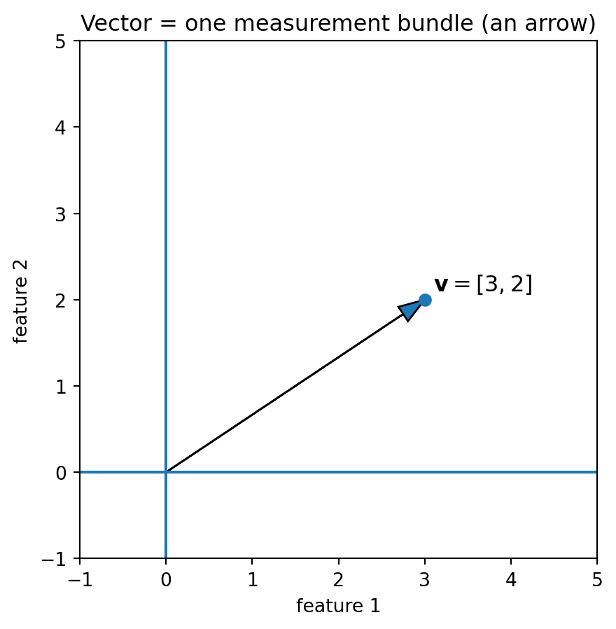
  • Vector: an ordered list of numbers that represent one thing with multiple measurements.
    Example: \(x = [\text{gpa},\text{test},\text{extra}]\).

  • Dot product: a way to combine two vectors to get a single number that tells how much the vectors point in the same direction. Intuition: “How aligned is \(x\) with direction \(w\)?”

1. Conceptual scaffold

Vectors and Matrices

  • All of modern data science is about structured combinations of numbers.
    • ↗ Vectors = single measurements
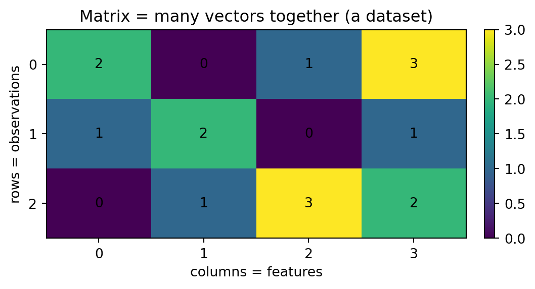
    • 🧮 Matrices = collections of measurements
    • ⚙️ Linear ops = controlled ways of mixing them
Code
import numpy as np
import matplotlib.pyplot as plt

v = np.array([3, 2])

fig, ax = plt.subplots(figsize=(5, 5))
ax.set_aspect("equal", adjustable="box")
ax.set_xlim(-1, 5)
ax.set_ylim(-1, 5)

# axes
ax.axhline(0)
ax.axvline(0)

# vector arrow
ax.arrow(0, 0, v[0], v[1], length_includes_head=True, head_width=0.2)
ax.scatter([v[0]], [v[1]])

ax.text(v[0] + 0.1, v[1] + 0.1, r"$\mathbf{v}=[3,2]$", fontsize=12)

ax.set_title("Vector = one measurement bundle (an arrow)")
ax.set_xlabel("feature 1")
ax.set_ylabel("feature 2")

plt.show()
Code
import numpy as np
import matplotlib.pyplot as plt

X = np.array([
    [2, 0, 1, 3],
    [1, 2, 0, 1],
    [0, 1, 3, 2],
])

fig, ax = plt.subplots(figsize=(6, 2.8))
im = ax.imshow(X, aspect="auto")

# annotate numbers
for i in range(X.shape[0]):
    for j in range(X.shape[1]):
        ax.text(j, i, str(X[i, j]), ha="center", va="center")

ax.set_title("Matrix = many vectors together (a dataset)")
ax.set_xlabel("columns = features")
ax.set_ylabel("rows = observations")

ax.set_xticks(range(X.shape[1]))
ax.set_yticks(range(X.shape[0]))

plt.colorbar(im, ax=ax, fraction=0.03, pad=0.04)
plt.show()

Note

Almost every dataset you will ever analyze — images, text embeddings, survey responses — lives in one object: a matrix

Norms!

  • A norm is a way to measure how “large” or “long” a vector is.

    • It takes a vector \(x\) and returns a non-negative number \(\lVert x\rVert\).
  • For \(x \in \mathbb{R}^d\), the \(p\)-norm is \[ \lVert x\rVert_p = \left( \sum_{i=1}^d |x_i|^p \right)^{1/p}. \]

  • Common special cases:

    • Euclidean norm (length): \[ \|x\|_2 = \sqrt{x_1^2 + x_2^2 + \dots + x_d^2}. \]
    • Manhattan norm: \[ \|x\|_1 = \sum_{i=1}^d |x_i|. \]
    • Max norm: \[ \|x\|_\infty = \max_{1 \le i \le d} |x_i|. \]
  • In this course, when we write \(\|x\|\) with no subscript, we mean the Euclidean norm \(\|x\|_2\).

Agreement and weighted scores

We want to turn “how good a fit is this applicant?” into a single number we can use for decisions.

  • Each applicant is a feature vector \[ \mathbf{x} = [\text{gpa},\ \text{test},\ \text{extra}]. \]
  • The committee’s priorities are a weight vector \[ \mathbf{w} = [w_{\text{gpa}},\ w_{\text{test}},\ w_{\text{extra}}]. \]
  • We seek a measure that we’ll define like this: \[ \boxed{\text{score}(\mathbf{x}) = \mathbf{x}\cdot\mathbf{w} + b}. \]

Here, the dot product, \(\boxed{x\cdot y}\) will do two jobs at once:

  1. It will combine features with weights into one score.
  2. It will measure how much \(\mathbf{x}\) points in the same direction as \(\mathbf{w}\).

Unit vectors: seeing \(\theta\) and \(\cos\theta\)

To build intuition, start with unit vectors in 2D:

  • Fix \(\mathbf{x}\) along the horizontal axis with length \(\lVert x \rVert = 1\).
  • Rotate another unit vector \(\mathbf{y}\) through different angles \(\theta\).
  • Watch how the projection of \(\mathbf{y}\) on \(\mathbf{x}\) and \(\cos\theta\) move together.
  • Why this makes sense with our picture:
    • θ ≈ 0° → vectors point the same way → cos θ ≈ 1 → full length
    • θ ≈ 90° → vectors are perpendicular → cos θ ≈ 0 → no projection
    • θ ≈ 180° → vectors point opposite ways → cos θ ≈ −1 → full length, flipped

Important

So far, \(x \cdot y = \cos \theta\) is our dot product for two vectors of unit length.

For unit vectors, \(x \cdot y \in [-1,1]\), which measures agreement in direction.

2. Math lens

Projection

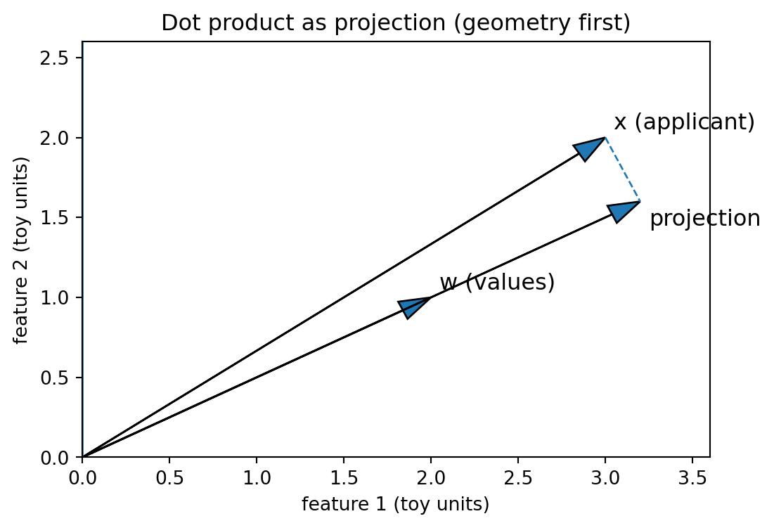
  • The projection of \(\mathbf{y}\) onto \(\mathbf{x}\) is the “shadow” of \(\mathbf{y}\) along the direction of \(\mathbf{x}\).

  • When \(\lVert\mathbf{x}\rVert = \lVert\mathbf{y}\rVert = 1\), the length of the shadow is \(\cos\theta\).

  • What if \(\lVert y \rVert \neq 1\)?

    • Use the sliders to change the length of \(\mathbf{y}\) and the angle \(\theta\).
  • Remember that for right-angle triangles: \[ \cos \theta = \frac{\text{adjacent}}{\text{hypotenuse}} \]
    • Here, the adjacent side is the shadow of \(\mathbf{y}\) along \(\mathbf{x}\).
    • The hypotenuse is the length of \(\mathbf{y}\), \(\lVert y \rVert\).
  • So the projection length, i.e., the amount of agreement, when \(\lVert x \rVert=1\) is: \[ x \cdot y = \lVert y \rVert \cos \theta \]
  • But \(\lVert x \lVert\) can also vary. This just scales our amount of ‘agreement’, and we’ve reached our goal, the general form of the ‘dot product’:

\[ \boxed{ \mathbf{x} \cdot \mathbf{y} = \lVert\mathbf{x}\rVert\,(\underbrace{\lVert\mathbf{y}\rVert\cos\theta}_{\text{shadow of } \mathbf{y} \text{ along } \mathbf{x}})} \]

Same picture in 3D

In 3D, nothing conceptually changes:

  • Vectors are arrows in 3D space.
  • There is still a single angle \(\theta\) between them.
  • The same rule holds: \[ \mathbf{x}\cdot\mathbf{y} = \lVert\mathbf{x}\rVert\,\lVert\mathbf{y}\rVert \cos\theta. \]

The plot below keeps \(\mathbf{x}\) fixed and rotates \(\mathbf{y}\) in a plane that contains \(\mathbf{x}\), so we can still see the angle and projection clearly.

🔬 From geometry to the coordinate rule

Our geometric rule

\[ \mathbf{x}\cdot\mathbf{y} = \lVert\mathbf{x}\rVert\,\lVert\mathbf{y}\rVert \cos\theta \]

explains angle and length. Now we want a simple coordinate formula that matches this picture.

Take 2D vectors

\[ \mathbf{x} = [x_1, x_2], \qquad \mathbf{y} = [y_1, y_2]. \]

  1. Their lengths come from Pythagoras: \[ \lVert\mathbf{x}\rVert^2 = \sqrt{x_1^2 + x_2^2}, \quad \lVert\mathbf{y}\rVert^2 = \sqrt{y_1^2 + y_2^2}. \]
  2. The distance between them is \[ \lVert\mathbf{x}-\mathbf{y}\rVert^2 = \sqrt{(x_1 - y_1)^2 + (x_2 - y_2)^2}. \]
  3. But that same distance is also related to the angle at the origin: \[ \lVert\mathbf{x}-\mathbf{y}\rVert^2 = \lVert\mathbf{x}\rVert^2 + \lVert\mathbf{y}\rVert^2 - 2\,\lVert\mathbf{x}\rVert\,\lVert\mathbf{y}\rVert\cos\theta. \] (This is just the cosine rule for triangles.)

If we now expand both sides in coordinates and match terms, the “mystery quantity”

\[ \lVert\mathbf{x}\rVert\,\lVert\mathbf{y}\rVert\cos\theta \]

has to be

\[ x_1y_1 + x_2y_2. \]

That motivates the coordinate definition of the dot product:

\[ \mathbf{x}\cdot\mathbf{y} = x_1y_1 + x_2y_2 \]

and in \(d\) dimensions,

\[ \boxed{\mathbf{x}\cdot\mathbf{y} = \sum_{i=1}^d x_i y_i}. \]

Dot product: the rule

For two \(d\)-dimensional vectors

\[ x = [x_1, x_2, \ldots, x_d], \quad w = [w_1, w_2, \ldots, w_d] \]

their dot product is

\[ \begin{align} w \cdot x &= \sum_{i=1}^d w_i x_i\\ &= w_1 x_1 + w_2 x_2 + \ldots + w_d x_d\\ &= x \cdot w \end{align} \]

From geometry to data science

We derived two ways to view the same score, \(x\cdot y\), but we stopped short of defining a full projection – the actual vector object produced by projecting one vector on another.

Why do we care so much about projections?

  • Similarity of data points
    • Cosine similarity between feature vectors is based on the dot product.
  • Linear regression
    • The best-fit line is literally a projection of the target onto the space spanned by the features.
  • Dimensionality reduction (e.g., PCA)
    • We project high-dimensional data onto a smaller number of important directions.

One-sentence wrap-up

Important

The dot product measures how much one vector acts in the direction of another;

It is a symmetric measure of similarity between two vectors, scaled by their lengths, with \(\cos\theta\) telling us the directional fraction.

3. Example: “Admissions as geometry”

Tiny numeric example

Suppose

  • gpa = 3.2, test_score = 80, extracurriculars = 2
  • w = [18, 0.6, 2.5], b = -20

Then

\[ \begin{aligned} w \cdot x &= 18(3.2) + 0.6(80) + 2.5(2) \\ &= 57.6 + 48 + 5 = 110.6 \\ \text{score} &= w \cdot x + b= 110.6 -20 = 90.6 \end{aligned} \]

So this applicant gets a score of about 90.6 under this rule.

Later we’ll:

  • use this score to compare applicants
  • compare this rule to a baseline (e.g., always predict the mean).

Geometry view

❌ anti-example: naïve ordinal “encoding”

  • Suppose we code extracurricular intensity as:
    • none=0, some=1, lots=2
  • This implies distances (2 is twice 1) that may not be real.
  • Vectors force you to ask: what does arithmetic mean here?

Generate the admissions dataset

Code
import numpy as np
import pandas as pd

rng = np.random.default_rng(1109)
n = 800

gpa = np.clip(rng.normal(3.0, 0.5, n), 0, 4)
test_score = np.clip(rng.normal(70, 12, n), 0, 100)
extracurriculars = np.clip(rng.poisson(2.0, n), 0, 10)

w_true = np.array([18.0, 0.6, 2.5])  # weights for [gpa, test_score, extracurriculars]
b_true = -20.0
noise = rng.normal(0, 6.0, n)

X = np.column_stack([gpa, test_score, extracurriculars])
admit_score = np.clip(b_true + X @ w_true + noise, 0, 100)

df = pd.DataFrame({
    "gpa": gpa,
    "test_score": test_score,
    "extracurriculars": extracurriculars,
    "admit_score": admit_score
})

df.head()
gpa test_score extracurriculars admit_score
0 2.914914 74.102432 0 84.763735
1 3.241503 75.086704 1 73.784401
2 3.104488 82.824867 1 77.304985
3 2.985164 74.637932 1 83.841901
4 2.095639 67.495786 4 71.320334

🐍

This code implements the dot product by multiplying vecotrs X and w_true using 🔗 @

Score one applicant + show contributions

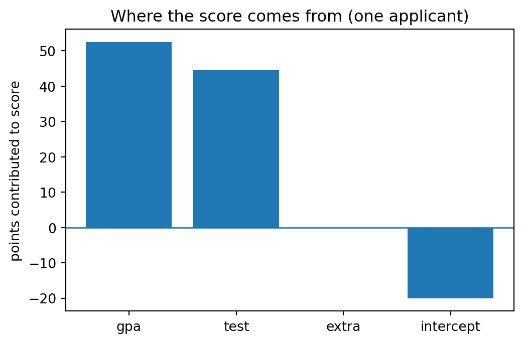
Consider the first applicant, represented by the first row of that table.

Code
idx = 0
x = df.loc[idx, ["gpa","test_score","extracurriculars"]].to_numpy()
score = b_true + np.dot(w_true, x)

contrib = pd.DataFrame({
    "feature": ["gpa","test_score","extracurriculars"],
    "x": x,
    "w": w_true,
    "w * x": w_true * x
})
contrib.loc["intercept", :] = ["(intercept)", np.nan, np.nan, b_true]
contrib
feature x w w * x
0 gpa 2.914914 18.0 52.468452
1 test_score 74.102432 0.6 44.461459
2 extracurriculars 0.000000 2.5 0.000000
intercept (intercept) NaN NaN -20.000000

Predicted score (no noise): 76.9
Observed admit_score (with noise): 84.8

Matrix form beats loops

Rather than compute each score row-by-row in a for loop, just use our matrix multiplier once, over the entire matrix.

This is elegant and simple.

Code
X = df[["gpa","test_score","extracurriculars"]].to_numpy()  # shape (n, d)
w = w_true                                                   # shape (d,)
b = b_true

y_hat_vec = b + X @ w                # (n,)  ✅
y_hat_vec[:5]
array([76.92991124, 85.89907162, 88.07570349, 81.01570466, 68.21897329])

A loop baseline

Code
y_hat_loop = []
for i in range(X.shape[0]):
    y_hat_loop.append(b + np.dot(X[i], w))
y_hat_loop = np.array(y_hat_loop)

np.max(np.abs(y_hat_vec - y_hat_loop))
0.0

Note

Baseline approach works (there’s no numerical difference with the ‘matrix form’), but its relative complexity might induce bugs, and it hides the algebra.

Severe test mindset: a train/test split

We’re not fitting yet – our ‘baseline’ is just the average on the ‘train’ data and our ‘rule’ is just the dot-product from before.

We’re just practicing the habit of not “testing” on the same data we tuned on.

Code
from sklearn.model_selection import train_test_split

train_idx, test_idx = train_test_split(np.arange(len(df)), test_size=0.25, random_state=1109)

y = df["admit_score"].to_numpy()
y_hat = y_hat_vec

def mse(a, b):
    return float(np.mean((a-b)**2))

baseline = np.mean(y[train_idx])                # mean predictor baseline (trained on train only)
y_base = np.full_like(y[test_idx], baseline)

mse_base = mse(y[test_idx], y_base)
mse_rule = mse(y[test_idx], y_hat[test_idx])

pd.DataFrame({
    "model": ["Baseline: predict mean(train)", "Linear rule (known weights)"],
    "MSE on test": [mse_base, mse_rule]
})
model MSE on test
0 Baseline: predict mean(train) 138.225821
1 Linear rule (known weights) 37.367713

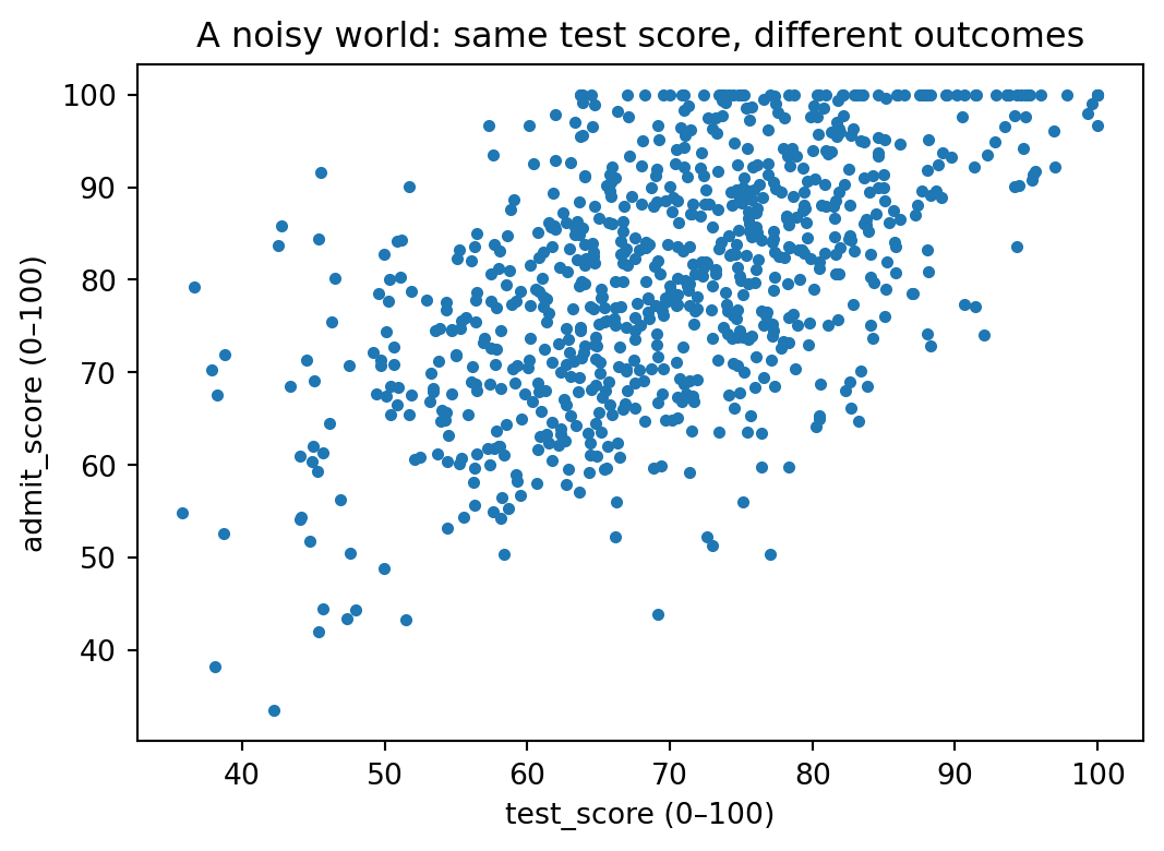
Visual: what does the rule “look like”?

Note

No single variable fully determines real-world outcomes.

Even with the same test_score, outcomes differ due to other factors and randomness.

Broadcasting an intercept to every prediction

Broadcasting is NumPy’s rule for applying element-wise operations to arrays of different shapes by implicitly expanding dimensions to make them compatible.

If y_hat has shape (n,), then b is a scalar and broadcasting is safe: NumPy repeats b n times implicitly.

  • The trap: subtracting a mean along the wrong axis.
    • Here we “center” the data two different ways: correctly by subtracting each column’s mean, and incorrectly (but valid via broadcasting) by subtracting each row’s mean—changing the meaning of the data.
Code
X = df[["gpa","test_score","extracurriculars"]].to_numpy()

mu_features = X.mean(axis=0)   # shape (d,)
X_centered = X - mu_features   # ✅ subtract per-column means

mu_rows = X.mean(axis=1)       # shape (n,)
# X - mu_rows would ERROR (shapes don't align) unless reshaped
mu_rows_col = mu_rows.reshape(-1, 1)  # shape (n,1)
X_centered_wrong = X - mu_rows_col    # ⚠️ subtract per-row mean (different meaning!)

pd.DataFrame({
    "gpa_centered_ok": X_centered[:5,0],
    "gpa_centered_wrong": X_centered_wrong[:5,0]
})
gpa_centered_ok gpa_centered_wrong
0 -0.074894 -22.757535
1 0.251694 -23.201233
2 0.114680 -25.871964
3 -0.004645 -23.222535
4 -0.894169 -22.434836

Metric choice revisited

If this score is used to rank applicants for review, we care about ranking quality and error size.

For now, we use MSE as a simple severity-of-error metric (large mistakes are worse than small ones).

Later, if we threshold into admit/reject, we’ll use precision/recall because false negatives and false positives have different costs.

Ethics nudge

  • As always, these simple examples can hide ethical gaps.
    • Opportunity bias: extracurricular count can proxy access to resources; treat it as measurement with context, not “merit”.
    • Transparency isn’t neutrality: a linear rule is easy to explain, but it still encodes values without exception.
  • Mitigation mindset:
    • document the intended use (“prioritize review”), and run subgroup checks once you have subgroup labels ethically collected.

Quick check

Q1

If X has shape (800, 3) and w has shape (3,), what shape is X @ w?

  1. (800, 3)
  2. (800,)
  3. (3,)
  4. scalar

Q2

Which is a good reason to use a baseline?

  1. To make your model look better
  2. To check if your effort beats something trivial
  3. Because it’s required by NumPy
  4. To avoid train/test splits

Q3

You subtract X.mean(axis=1).reshape(-1,1) from X. What did you center?

  1. Each feature (column) around 0
  2. Each applicant (row) around 0
  3. Nothing (broadcasting fails)
  4. The intercept only

Q4

Why is “extracurriculars=2 is twice extracurriculars=1” potentially dangerous?

  1. Because dot products can’t handle integers
  2. Because counts always violate fairness
  3. Because it assumes a numeric distance meaning that may not match reality
  4. Because matrices must be square