“Clone” rows from systems that sync badly (duplicates)
Extreme points that might be mistakes… or the most important cases (outliers)
If you ignore these, your model will happily learn patterns in:
typos,
broken sensors,
and half-recorded events.
This module is about learning to notice and question those problems before they quietly wreck your conclusions.
High-level data quality
Some useful lenses:
Accuracy – does the value reflect reality?
Precision – how finely is it measured?
Completeness – which values are simply not there?
Consistency – are formats / units / states aligned?
Timeliness – is the data current enough?
Believability – do we trust who and how it was recorded?
Interpretability – can humans understand it?
Five flavours of dirty data
You will see these constantly:
Inconsistent types
Inconsistent values
Missing data
Outliers
Noise and recording errors (including wrong labels)
We’ll anchor everything on a small, fictional dataset.
Campus Wellness Check-ins
Students can do quick wellness check-ins at kiosks (residences, gym). Clinic staff enter some records later. Two different systems get merged weekly.
Each row = one check-in event.
Variables:
checkin_id (string; sometimes missing from one system)
student_hash (pseudonymous ID, stable per student)
timestamp (when the check-in happened)
location ∈ {ResidenceA, ResidenceB, Gym, Clinic}
sleep_hours_last_night (float)
stress_1to10 (int; 1=low, 10=high)
temp_c (float; should be Celsius)
resting_hr (int; beats per minute)
notes (free text, often messy)
Tiny sample of the data
Code
import pandas as pdimport numpy as nprows = [ {"checkin_id":"A-0001","student_hash":"S_19f","timestamp":"2025-01-11 09:02","location":"ResidenceA","sleep_hours_last_night":7.5,"stress_1to10":3,"temp_c":36.8,"resting_hr":62,"notes":""}, {"checkin_id":"A-0002","student_hash":"S_19f","timestamp":"2025-01-12 09:01","location":"ResidenceA","sleep_hours_last_night":np.nan,"stress_1to10":-1,"temp_c":36.7,"resting_hr":61,"notes":"skipped sleep/stress"}, {"checkin_id":"B-1148","student_hash":"S_9aa","timestamp":"2025-01-12 17:40","location":"Gym","sleep_hours_last_night":6.0,"stress_1to10":6,"temp_c":98.2,"resting_hr":72,"notes":"temp entered in F?"}, {"checkin_id":"C-0104","student_hash":"S_0c2","timestamp":"2025-01-13 12:15","location":"Clinic","sleep_hours_last_night":5.0,"stress_1to10":9,"temp_c":37.9,"resting_hr":240,"notes":"device glitch?"}, {"checkin_id":None,"student_hash":"S_0c2","timestamp":"2025-01-13 12:16","location":"Clinic","sleep_hours_last_night":5.0,"stress_1to10":9,"temp_c":37.9,"resting_hr":120,"notes":"manual entry (no id)"}, {"checkin_id":"B-1150","student_hash":"S_7d1","timestamp":"2025-01-14 08:58","location":"ResidenceB","sleep_hours_last_night":26.0,"stress_1to10":2,"temp_c":36.5,"resting_hr":58,"notes":"impossible sleep"}, {"checkin_id":"A-0008","student_hash":"S_5b8","timestamp":"2025-01-14 09:05","location":"ResidenceA","sleep_hours_last_night":8.0,"stress_1to10":0,"temp_c":36.6,"resting_hr":0,"notes":"sensor dropout"}, {"checkin_id":"B-1151","student_hash":"S_9aa","timestamp":"2025-01-12 17:40","location":"Gym","sleep_hours_last_night":6.0,"stress_1to10":6,"temp_c":98.2,"resting_hr":72,"notes":"duplicate from merge"}]df_tiny = pd.DataFrame(rows)df_tiny
checkin_id
student_hash
timestamp
location
sleep_hours_last_night
stress_1to10
temp_c
resting_hr
notes
0
A-0001
S_19f
2025-01-11 09:02
ResidenceA
7.5
3
36.8
62
1
A-0002
S_19f
2025-01-12 09:01
ResidenceA
NaN
-1
36.7
61
skipped sleep/stress
2
B-1148
S_9aa
2025-01-12 17:40
Gym
6.0
6
98.2
72
temp entered in F?
3
C-0104
S_0c2
2025-01-13 12:15
Clinic
5.0
9
37.9
240
device glitch?
4
None
S_0c2
2025-01-13 12:16
Clinic
5.0
9
37.9
120
manual entry (no id)
5
B-1150
S_7d1
2025-01-14 08:58
ResidenceB
26.0
2
36.5
58
impossible sleep
6
A-0008
S_5b8
2025-01-14 09:05
ResidenceA
8.0
0
36.6
0
sensor dropout
7
B-1151
S_9aa
2025-01-12 17:40
Gym
6.0
6
98.2
72
duplicate from merge
Spot the problems
From that tiny table we already see:
Missing fields
sleep_hours_last_night = NaN
checkin_id = None
Off-script “fake” values
stress_1to10 = -1, stress_1to10 = 0 used as “missing”
Unit mistakes
temp_c = 98.2 is probably Fahrenheit (an archaic form of measurement)
Sensor glitches
resting_hr = 0, 240
Duplicates
Same student & timestamp from the weekly merge
Examples like these are common.
Missingness
Missing data: the easy cases
“Easy” missingness is visible in the table:
Explicit nulls (NaN, None, empty strings)
Impossible placeholders used for missing:
age = -1, age = 999
stress_1to10 = -1 in our dataset
"unknown", "N/A" etc
These are perfect targets for easy automations we’ll see shortly.
Missing data: harder to see
Sometimes missingness is not obvious:
A person is dropped from the database entirely
(how would you even know?)
One system always leaves checkin_id blank, another always fills it
Staff sometimes skip certain questions under pressure
Different hospitals / apps log different subsets of fields
Visible values can encode invisible decisions about what was or was not recorded.
Three ways missingness happens
Classic categories:
MCAR – Missing Completely At Random
e.g., kiosk offline randomly; some rows lost independent of values.
MAR – Missing At Random (given other observed variables)
e.g., clinic staff always fill all fields; gym kiosks skip temp_c.
MNAR – Missing Not At Random
e.g., people with highest stress skip the stress_1to10 field.
In practice, you often guess which regime you are closest to, based on domain knowledge.
When missingness is actually information
Sometimes “no value recorded” is the value. 😮
In EHRs, whether a lab was ever ordered can be more predictive than the lab value itself
Example: patients with no cholesterol test often have lower cardiovascular risk, because the clinician never felt worried enough to order it. (Groenwold 2020)
Patterns where labs stop being ordered after a normal result can encode disease severity and clinical reassurance. These “informatively missing” labs have been used to stratify COVID-19 inpatients across multiple hospital systems. (Tan et al. 2023)
For many common labs, missingness is tied to disease burden: sicker patients get more labs (less missingness), while healthier patients often have more gaps in their records. (Li et al. 2021)
In prediction models built from EHRs, one strategy is to keep missingness as a feature:
add binary “missing indicator” variables that mark when a predictor is absent. Simulation work shows that, when missingness is informative, indicators can sometimes improve or at least not harm model performance. (Ehrig et al. 2025; Wells et al. 2013)
Take-home
Don’t always rush to “fill in the blanks.” For some variables, “not measured” is itself a signal about clinical judgment, workflow, and patient state — but that signal can change once we start using it in deployed models.
The missing entry in x3 is replaced with the average of the two closest rows (in the space of x1, x2, x4).
Outliers
Outliers: what are they?
Intuitively:
An outlier is a datapoint that differs strongly from most others.
Common causes:
Measurement error (e.g., HR = 0, 240)
Unit errors (98.2°F in a “Celsius” column)
Rare but real events (post-workout HR of 160)
New phenomena (a truly unusual case)
There is no single perfect definition.
For “nice” distributions, a common rule of thumb is: more than 3 standard deviations from the mean.
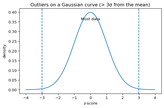
Outliers on a Gaussian curve
For a Normal distribution:
~68% of data lies within 1σ of the mean
~95% within 2σ
~99.7% within 3σ
Anything beyond ±3σ is very rare (~0.3% total):
Code
import numpy as npimport matplotlib.pyplot as pltfrom math import exp, pi, sqrtx = np.linspace(-4,4,400)y = (1/np.sqrt(2*pi)) * np.exp(-0.5* x**2)plt.figure(figsize=(6,4))plt.plot(x,y)plt.axvline(-3, linestyle="--")plt.axvline(3, linestyle="--")plt.text(0, max(y)*0.9, "Most data", ha="center")plt.xlabel("z-score")plt.ylabel("density")plt.title("Outliers on a Gaussian curve (> 3σ from the mean)")plt.tight_layout()
Points out in the thin tails are candidates for outliers — but context still matters.
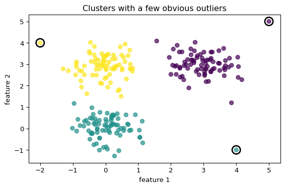
Outliers via clustering (preview)
We can also spot outliers with clustering (later module):
Imagine grouping points into clusters.
Points that are:
far from every cluster centre, or
stuck in very tiny clusters
are candidates for outliers.
This works even when the data are not nicely Normal, but depends on the clustering algorithm and distance measures.
Code
import numpy as npimport matplotlib.pyplot as pltfrom sklearn.cluster import KMeansnp.random.seed(1109)# Three compact clusterscluster1 = np.random.normal(loc=[0, 0], scale=0.5, size=(80, 2))cluster2 = np.random.normal(loc=[3, 3], scale=0.5, size=(80, 2))cluster3 = np.random.normal(loc=[0, 3], scale=0.5, size=(80, 2))X = np.vstack([cluster1, cluster2, cluster3])# A few obvious outliersoutliers = np.array([[5, 5], [4, -1], [-2, 4]])X_all = np.vstack([X, outliers])# Fit k-means with 3 clusterskmeans = KMeans(n_clusters=3, n_init="auto", random_state=1109)labels = kmeans.fit_predict(X_all)plt.figure(figsize=(6, 4))# Plot all points coloured by clusterplt.scatter(X_all[:, 0], X_all[:, 1], c=labels, alpha=0.7)# Highlight the injected outliers with big hollow markersplt.scatter(outliers[:, 0], outliers[:, 1], s=150, facecolors="none", edgecolors="black", linewidths=2)plt.xlabel("feature 1")plt.ylabel("feature 2")plt.title("Clusters with a few obvious outliers")plt.tight_layout()
🕵️♀️ Handling outliers: choices
Common strategies:
Investigate & fix actual errors
(e.g., convert Fahrenheit to Celsius)
Treat as missing when clearly wrong
(e.g., HR = 0 → missing HR)
Clip extreme values to a reasonable range
Transform (e.g., log transform for heavy-tailed data)
Use robust models that downweight outliers
Model them separately
(e.g., anomaly-detection task)
Deleting outliers blindly can erase exactly the events you want to discover.
Interactive demo: HR outliers over time
We’ll use a slightly larger synthetic sample of resting heart rate from our campus dataset and see how changing the “outlier rule” changes which points are flagged.
Noisy labels → multiple annotators and agreement measures.
Outliers can be wrong, rare, or the most interesting part.
Flag, inspect, and decide — don’t just delete.
Duplicates require a definition of “same entity, same event”.
Before modeling, always ask:
What’s missing, and why might it be missing?
Where could there be duplicates?
Which values look impossible or suspicious?
What cleaning choices might change my conclusions?
Later modules will build on this: scaling, encoding, binning, and more advanced feature engineering.
References
Ehrig, Molly, Garrett S. Bullock, Xiaoyan Iris Leng, Nicholas M. Pajewski, and Jaime Lynn Speiser. 2025. “Imputation and Missing Indicators for Handling Missing Longitudinal Data: Data Simulation Analysis Based on Electronic Health Record Data.”JMIR Medical Informatics 13: e64354. https://doi.org/10.2196/64354.
Groenwold, Rolf H. H. 2020. “Informative Missingness in Electronic Health Record Systems: The Curse of Knowing.”Diagnostic and Prognostic Research 4 (8): 8. https://doi.org/10.1186/s41512-020-00077-0.
Li, Jiang, Xiaowei S. Yan, Durgesh Chaudhary, Venkatesh Avula, Satish Mudiganti, Hannah Husby, et al. 2021. “Imputation of Missing Values for Electronic Health Record Laboratory Data.”Npj Digital Medicine 4: 147. https://doi.org/10.1038/s41746-021-00518-0.
Tan, Amelia L. M., Emily J. Getzen, Meghan R. Hutch, Zachary H. Strasser, et al. 2023. “Informative Missingness: What Can We Learn from Patterns in Missing Laboratory Data in the Electronic Health Record?”Journal of Biomedical Informatics 139: 104306. https://doi.org/10.1016/j.jbi.2023.104306.
Wells, Brian J., Kevin M. Chagin, Amy S. Nowacki, and Michael W. Kattan. 2013. “Strategies for Handling Missing Data in Electronic Health Record Derived Data.”EGEMS (Washington, DC) 1 (3): 1035. https://doi.org/10.13063/2327-9214.1035.