M02 - Python setup: notebooks, virtual env, conda

CSCI 1109 — Practical Data Science

Frank Rudzicz

Outcomes

  • Explain and compare virtual environments (venv, virtualenv, conda envs).
  • Configure Jupyter so the right kernel/interpreter is used.
  • Create a project env, run a notebook, and produce a plot and a table.
  • Export your environment for reproducibility and justify your choice.

⏱️ Setup now = analysis time later

  • If your environment breaks mid-assignment, you lose momentum and time
  • Today: 10 minutes of setup to save hours later

Tip

Rule of thumb: if something feels “annoying but small” in setup, it will become “huge and painful” at 1am before a deadline 😴.

Note

Goal for this module: you can reliably run notebooks, import packages, and know which Python is running your code.

🐍 Why Python for data science?

  • General-purpose language with rich scientific stack:
    • NumPy, pandas, Matplotlib, scikit-learn libraries.
  • Strong ecosystem (data wrangling, ML, visualization), great community and docs.
  • Pairs well with Jupyter notebooks and VS Code workflows.
    • We’ll discuss these soon
  • Caveats to respect: dynamic typing (add tests), slower tight loops (prefer 🔗 vectorization), version drift (pin envs).

Python and virtual environments

🤔 Do I already have Python?

Specifically, do you have v3?

  • 🚮 Windows (PowerShell or cmd)
    py -V OR python -V OR where python
  • 🍎 macOS / 🐧 Linux (Terminal)
    python3 --version OR which python3
  • Programmatic (paste into any Python):
import sys, platform
print(platform.python_version(), sys.executable)

If you see a version like 3.x and an interpreter path inside your project env (not system), you’re ready.

Install Python

Method Steps (summary) Best for Notes / Link
Python.org installer Download the Windows installer; run with “Add Python to PATH”; then py -V. Most users; simple local install. python.org → Windows
WinGet winget install -e --id Python.Python.3 (or latest id shown by winget search Python); restart shell; py -V. Admin-friendly, scriptable installs. WinGet docs
Miniforge (conda‑forge) Download Miniforge exe; install; conda create -n 1109 python=3.11 -y; conda activate 1109. Reproducible envs; class projects. Miniforge (conda‑forge)
Anaconda Distribution Download & install Anaconda; use Anaconda Prompt; manage envs with conda. GUI tools + many prebuilt pkgs. Anaconda Download
Method Steps (summary) Best for Notes / Link
Python.org pkg Download macOS installer; run; python3 --version. Simple, standalone install. python.org downloads
Homebrew brew install pythonpython3 --version. Devs already on Homebrew. Homebrew & Python
Miniforge (conda‑forge) Download .pkg or .sh; install; conda create -n 1109 python=3.11 -y; conda activate 1109. Repro envs; consistent with Windows/Linux. Miniforge
Anaconda Distribution Install Anaconda; manage envs with conda. All‑in‑one data science stack. Anaconda Download
Method Steps (summary) Best for Notes / Link
Ubuntu/Debian packages sudo apt update && sudo apt install -y python3 python3-venv python3-pip System-managed installs. Ubuntu dev guide (Python setup)
Fedora/RHEL packages sudo dnf install -y python3 python3-pip System-managed installs. Fedora docs on dnf
Arch btw sudo pacman -Syusudo pacman -S python python-pip → verify with python --version (use python -m venv .venv for project envs) Arch/Manjaro users comfortable with pacman Arch Wiki — Python
Miniforge (conda‑forge) Download installer; run bash Miniforge3-...sh; conda create -n 1109 python=3.11 -y; conda activate 1109. Isolated, reproducible envs across distros. Miniforge
Anaconda Distribution Download installer; bash Anaconda3-...sh; conda to manage envs. All‑in‑one stack & course parity. Anaconda Download

Package and isolate before we ship

  • Concrete pains you’ll hit without packaging
    • “Works on my machine”: graders/teammates/customers install slightly different builds → ❌ behaviour changes or breaks.
      • 👉 Packaging creates installable artifacts (e.g., 🔗 wheels) so others get the same code and compiled bits quickly and consistently.
    • Cross-project collisions: Project A needs pandas X; Project B needs pandas Y → ❌ one global install cannot satisfy both.
      • 👉 Per-project environments keep dependency trees separate.
    • Native libraries: Many data-science tools rely on BLAS/GDAL/CUDA, not just Python. We’ll soon see how to bundle these non-Python deps alongside Python packages (spoiler: Conda)

Package and isolate before we ship

  • Two jobs, two tools
    • Packaging answers: “How does someone else install what we built?”
      → Ship a distribution (prefer wheels) so installation is fast, reliable, and compatible across OS/architectures; publishing flows exist for this.
    • Environments answer: “Where does it run without breaking other projects?”
      → Isolate runtimes per project to prevent version conflicts and to reproduce results later.

Tip

Freeze what you run (package), isolate where you run it (env), and your work becomes reproducible, reviewable, and shippable.

Virtual environments (venv)

  • Why: isolate deps per project; avoid global installs.
  • Create & activate:
python -m venv .venv
# Windows: .\.venv\Scripts\activate
# macOS/Linux: source .venv/bin/activate
python -m pip install -U pip

Conda environments & channels

  • Conda manages packages + 🔗 environments (any language) and supports binary builds.
  • Create env, add pkgs, export:
conda create -n 1109-m02 python=3.11 pandas matplotlib -y
conda activate 1109-m02
conda env export --no-builds > environment.yml
  • 🔗 Channels determine package sources;
    • Many projects prefer 🔗 conda-forge for breadth + consistency.
  • Pip inside conda: install with conda first; then pip inside the activated env if needed; avoid mixing back-and-forth.

Conda gotcha

  • After conda init, Conda can auto-activate base whenever a shell opens. If you never deactivate it, your python/pip and Jupyter kernel default to base.
  • Why that’s a problem
    • Accidental installs into base: you think you’re installing for Project A, but pip/conda write into base. Later Project B breaks, or your notebook runs with the wrong packages.
    • Version collisions: base becomes a dumping ground; installing pandas vX for one project overwrites vY needed by another.
    • Repro headaches: “export the env” becomes messy—base now contains unrelated packages, channels, and versions.
# Stop auto-activating base on every new shell
conda config --set auto_activate_base false

# Create per-project envs (example)
conda create -n myproj python=3.11 -y
conda activate myproj

# Quick self-check
conda info --envs # active env has a * next to it (and shouldn’t be base for project work).
python -c "import sys; print(sys.executable)" #path should live in your project env.
pip --version # the path printed should also point into that same env.

venv vs conda

venv conda
What it is Per-project Python environment Environment + package manager
Package manager pip conda (you can add pip inside)
Non-Python deps No (uses system/toolchain) Yes (BLAS, HDF5, CUDA, …)
Binaries PyPI wheels; success varies by OS/toolchain Prebuilt, cross-platform binaries (e.g., conda-forge)
Repro artifact requirements.txt environment.yml
Ideal for Pure-Python stacks; lightweight apps; simple CI/CD Data-science stacks; geospatial/ML/GPU
Strengths Minimal, ubiquitous, standard Fewer compile headaches; consistent installs across OSs
Watch-outs Native builds can fail; system-pkg collisions Channel mixing; larger footprint; avoid always-on base

Note

Rule of thumb: If your project is pure-Python, prefer venv (+pip). If it’s binary-heavy or you need smooth cross-OS installs, prefer conda (ideally conda-forge). In both cases, export an env file so others can reproduce your results.

Post-install: create a project env

Two common routes — pick one per project.

A) venv (standard library)

python3 -m venv .venv
# macOS/Linux
source .venv/bin/activate
# Windows (PowerShell)
.\.venv\Scripts\Activate.ps1
python -m pip install -U pip # upgrades Pip in your env

→ Export later with python -m pip freeze > requirements.txt (PyPA guide).

B) conda (🔗 Miniforge / 🔗 Anaconda )

conda create -n 1109-m02 python=3.11 pandas matplotlib -y
conda activate 1109-m02
conda env export --no-builds > environment.yml

Development environments

Source files v Notebooks

  • Data science rarely happens in a straight line:

flowchart LR
    A("explore") -->|run|B("test")
    B -->|fix|A
    B --> C("explain")
    C --> |refactor|A    

  • A notebook keeps code, output, and reasoning side-by-side so analysis is transparent and replayable.
  • It replaces the “three-window problem”: script editor, terminal, and notes. In one interface you can run, inspect, and narrate.
  • A notebook is both a:
    • lab bench — you experiment interactively; variables persist while you explore.
    • lab notebook — you document what you did, why, and what you observed.
  • When shared, a notebook is an executable paper: others can re-run your steps and see the same evidence. It is not a shippable product

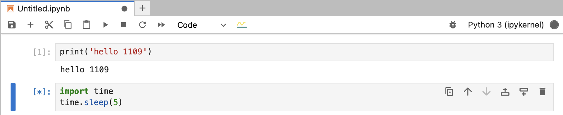
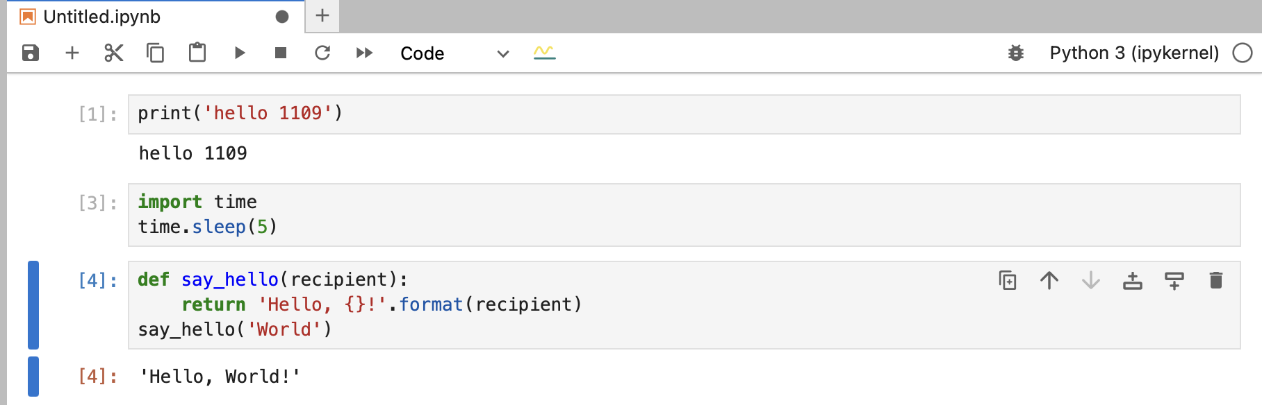
What is a .ipynb? + modes & shortcuts

  • A .ipynb is a JSON doc: ordered cells (markdown \(\oplus\) code) + outputs + metadata.
  • Two modes:
    • Edit (edit content)
    • Command (cell-level actions: render markdown \(\oplus\) execute code)

See 🔗 here

Shortcut crib (command mode)

Keys Action
A / B Insert cell Above / Below
M / Y Set cell to Markdown / Code
DD Delete cell
Shift-Enter Run & move down
Ctrl/Cmd-Enter Run in place

🧠 What is a Jupyter “kernel”?

---
config:
  look: handDrawn
  theme: neutral
  handDrawnSeed: 42      # optional, for reproducible scribbles
  fontSize: 36em
---
flowchart LR
  A["Notebook (.ipynb)"] -->|"sends code"| B["Kernel (specific Python env)"]
  B --> C["Packages (pandas, numpy, …)"]
  B --> D["Files + Data (csv, images,...)"]
  B --> E["Outputs (tables, plots, text)"]

  • If you pick the wrong kernel, your code may fail even if it “works on your friend’s laptop”
  • Most common symptom: ModuleNotFoundError (package isn’t installed in that kernel)

Tip

Always verify the kernel with sys.executable (it tells you which Python is running).

Code
import sys
print("Python executable:", sys.executable)
print("Python version:", sys.version.split()[0])
Python executable: /opt/homebrew/anaconda3/bin//python
Python version: 3.9.13
Code
# Optional: confirm key packages are coming from the same environment
import pandas as pd
import matplotlib
print("pandas:", pd.__version__)
print("matplotlib:", matplotlib.__version__)
pandas: 1.4.4
matplotlib: 3.5.2

Development environments

  • As in any free society, you have a choice of what development environment to use. E.g.:
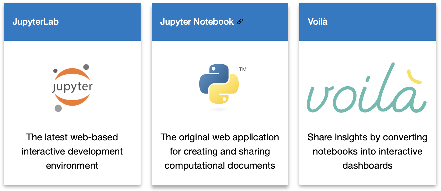
    1. Jupyter-lab
    2. VS Code
    3. Google Colab
    4. ⚠️ Emacs

1. Installing Jupyter

From 🔗 here

pip install jupyterlab # use the conda-forge channel
#or
brew install jupyterlab

# run it
jupyter-lab

1. Jupyter in practice — what runs where?

  • Launching Jupyter starts a local server on your machine (often http://localhost:8888) and opens a browser UI (dashboard → notebook).
  • The browser is the interface; the kernel (a local process) runs your code.
  • Closing the server shuts down its kernels; closing a notebook can also stop its kernel.

flowchart LR
  A["Browser UI"] -->|"HTTP/WebSocket"|B["Jupyter server (localhost)"]
  B --> |"kernel protocol"|C["Python kernel (your env)"]
  B --> D["File system: .ipynb, data, artifacts"]

2. VS Code

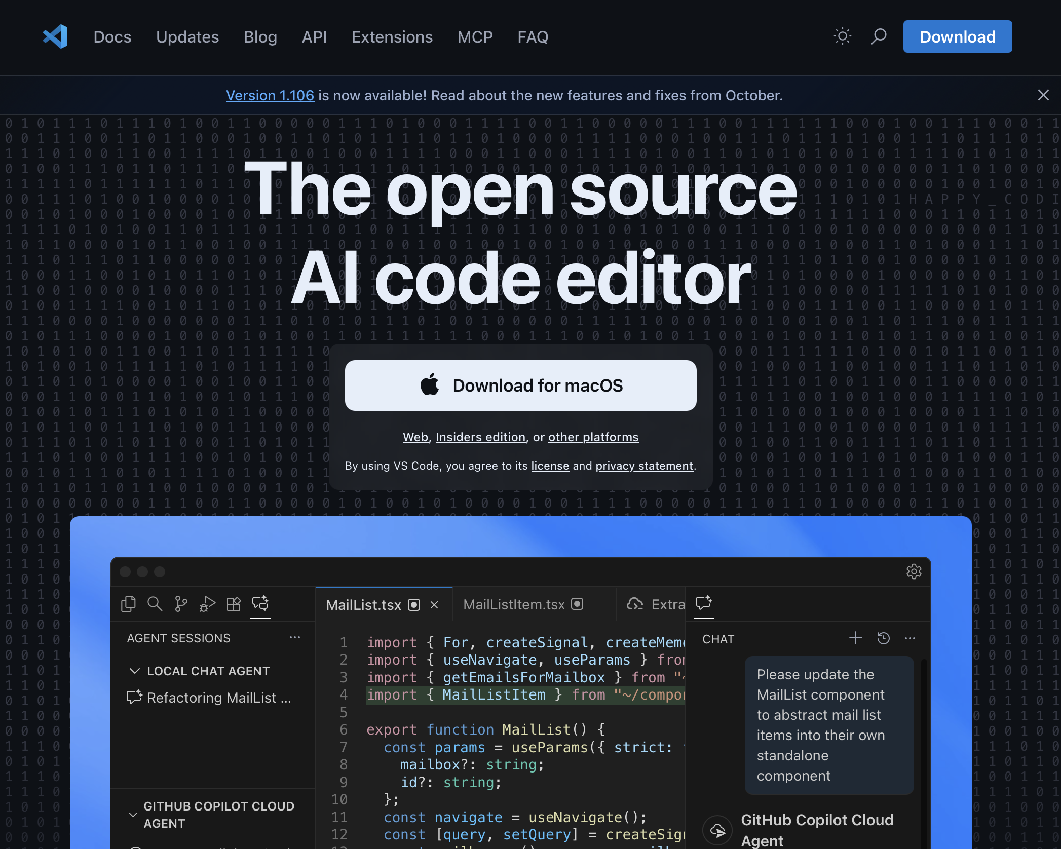
  • 🔗 VS Code is a popular free, open, multi-platform code editor
  • Interpreter selection drives kernel selection in VS Code. Use Python: Select Interpreter and read more 🔗 here
  • Jupyter architecture: front end ↔︎ server ↔︎ language kernels. 🔗 more on the back end
2. Verify your editor & kernel

  • In VS Code: Python: Select Interpreter should point to your project env.
  • In Jupyter: the notebook kernel should match that interpreter.
  • Quick sanity cell to run:
import sys, pandas as pd
print('python:', sys.version.split()[0], '\nexecutable:', sys.executable)
print('pandas:', pd.__version__)

3. Google Colab - Notebooks in the cloud

  • What it is: a hosted Jupyter environment from Google that runs through your browser.
  • Why it’s handy: fast setup, access to free GPUs/TPUs; computation happens in Google’s VM.
  • Best for: short-lived demos, workshops, assignments or when your local setup is broken.
  • Limits: sessions time out, storage is ephemeral (use Google Drive for persistence), and internet access may be restricted.
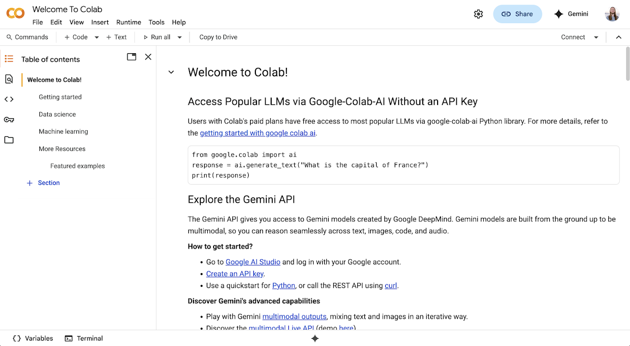
  • Reproducibility note: good for trying code, not ideal for shipping projects — always export notebooks + environment specs back to local version control.
  • 🔗 colab.research.google.com

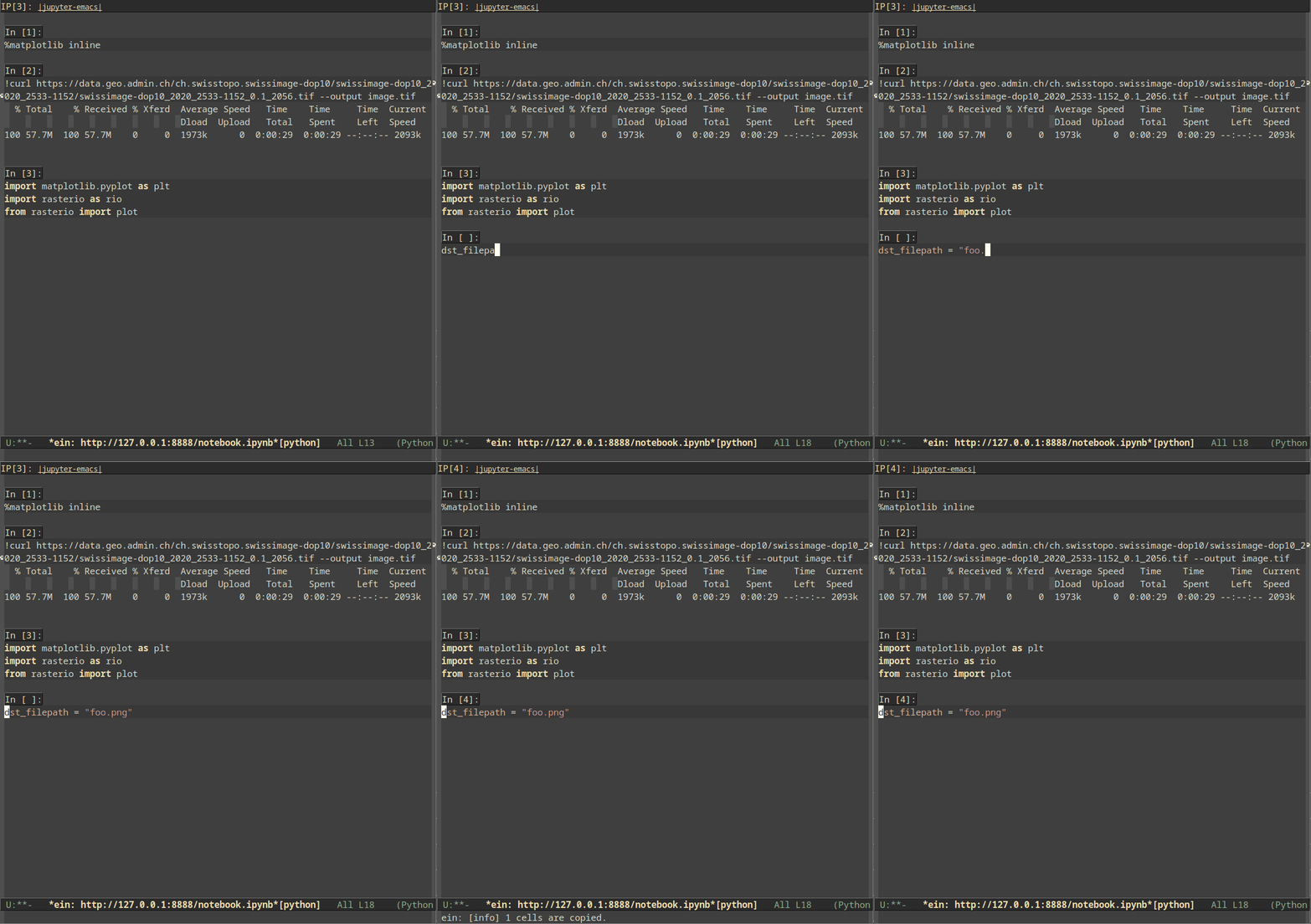
4. Emacs!

I love Emacs, the one true text editor.

As with all things, Jupyter notebooks run in Emacs too, but try this only if you’re playing life on 👷 Hard Mode.

See 🔗 Jupyter Emacs Universe and the 🔗 MELPA package
Toolchain & data flow

flowchart LR
  A["Project folder"] --> B["env.yml / requirements.txt"]
  B --> C{"Environment (venv or conda)"}
  C -->|"kernel spec"|D["Jupyter Kernel"]
  D --> E["Notebook (.ipynb)"]
  C --> F["Python Script (.py)"]
  E --> G["Artifacts: figures, tables"]
  F --> G
  C --> H["pip / conda"]
  H --> C 

  • Project folder is the home base: code, notebooks, and files.
  • env.yml (conda) \(\oplus\) requirements.txt (pip) describes what to install.
  • Environment (venv/conda) is the isolated Python you actually run. Install packages here with pip or conda—not globally.
  • Kernel spec (“kernel spec”) ties Jupyter to that environment.
  • Notebook (.ipynb) and script (.py) are just two front ends to the same environment—interactive vs. batch/CLI.
  • Artifacts (figures, tables) are outputs your code writes back into the project.
  • Feedback loop: if code errors about a missing package, install it in the env, then update env.yml/requirements.txt so others (and future you) can reproduce.

Examples

From data to decision

flowchart LR
  A["Raw data<br>(CSV/DB/URL)"] --> B["Clean & structure<br>(tidy units)"]
  B --> C["Compute<br>(features, summaries)"]
  C --> D["Visualize"]
  D --> E["Claim<br>(metric + uncertainty)"]
  E --> F["Decision<br> (cost-aligned)"]

1. Coffee demand vs temperature

Question: How does outside temperature relate to hot-drink orders (per day)?
Units: temp = °C; orders = count/day.

Code
import pandas as pd, numpy as np
import matplotlib.pyplot as plt
from io import StringIO

coffee = StringIO("""day,temp_C,orders
Mon, 3, 210
Tue, 5, 220
Wed, 7, 265
Thu, 9, 300
Fri,10, 340
Sat, 8, 310
Sun, 4, 250
""")

df = pd.read_csv(coffee)
df['orders_norm'] = df['orders'] / df['orders'].max()

print(df)

plt.figure(figsize=(6,4))
plt.scatter(df['temp_C'], df['orders'], s=80)
plt.title('Coffee orders vs temperature (°C)')
plt.xlabel('Temperature (°C)'); plt.ylabel('Orders / day')
plt.tight_layout(); plt.show()
   day  temp_C  orders  orders_norm
0  Mon       3     210     0.617647
1  Tue       5     220     0.647059
2  Wed       7     265     0.779412
3  Thu       9     300     0.882353
4  Fri      10     340     1.000000
5  Sat       8     310     0.911765
6  Sun       4     250     0.735294
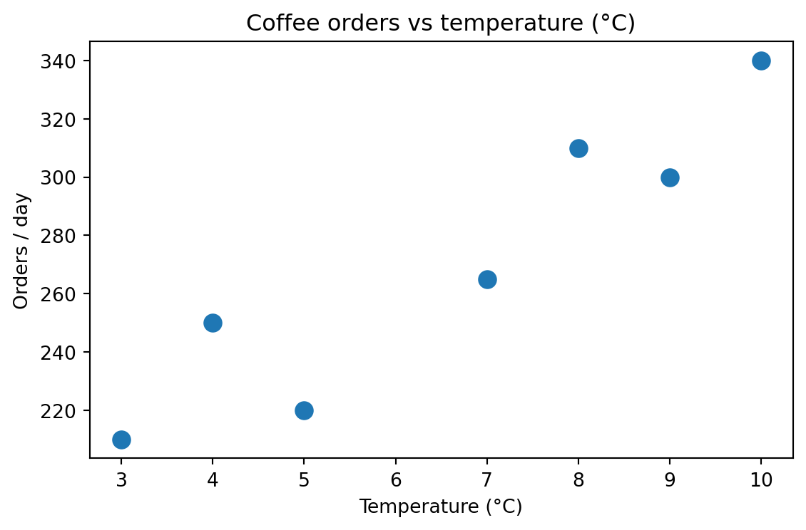
Interpretation prompt: Is the trend linear? What other variables might confound (weekday, rain, promotions)?
Decision hook: Stock & staffing decisions for chilly vs warm days.

2. Engagement over time

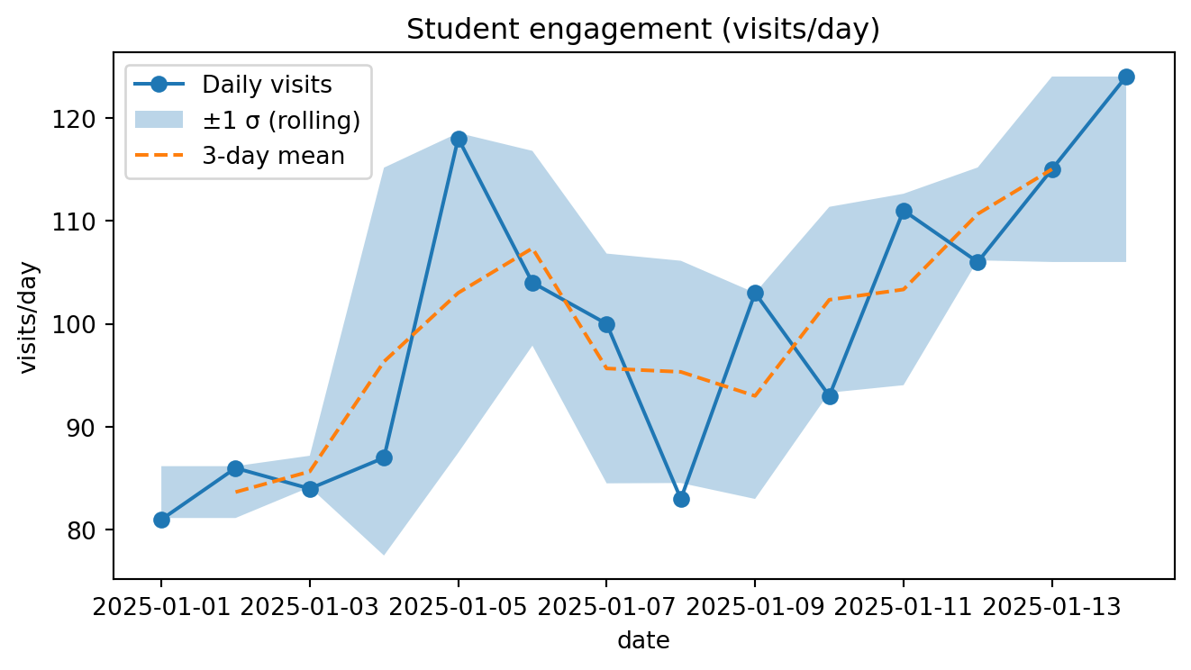
  • Let’s measure just visits / day
  • Noise (fluctuations) in these measurements can mask the signal (🤩the truth🤩)
  • We simulate 2 weeks of daily site visits and use a centered 3-day window.
    Units: visits = count/day.
Code
import pandas as pd, numpy as np, matplotlib.pyplot as plt
np.random.seed(0)

days = pd.date_range('2025-01-01', periods=14)
visits = np.random.poisson(lam=np.linspace(80,120,14))
df = pd.DataFrame({'date':days,'visits':visits})
df['roll3'] = df['visits'].rolling(3, center=True).mean()
df['band']  = df['visits'].rolling(3, center=True).std()

print(df.head())

plt.figure(figsize=(7,4))
plt.plot(df['date'], df['visits'], 'o-', label='Daily visits')
plt.fill_between(df['date'],
                 (df['roll3']-df['band']).fillna(method='bfill').fillna(method='ffill'),
                 (df['roll3']+df['band']).fillna(method='bfill').fillna(method='ffill'),
                 alpha=0.3, label='±1 σ (rolling)')
plt.plot(df['date'], df['roll3'], '--', label='3-day mean')
plt.legend(); plt.title('Student engagement (visits/day)')
plt.xlabel('date'); plt.ylabel('visits/day'); plt.tight_layout(); plt.show()
        date  visits       roll3       band
0 2025-01-01      81         NaN        NaN
1 2025-01-02      86   83.666667   2.516611
2 2025-01-03      84   85.666667   1.527525
3 2025-01-04      87   96.333333  18.823744
4 2025-01-05     118  103.000000  15.524175
Note

Takeaway: Smoothed trend ≠ ground truth; bands show local variability.
Decision hook: When to escalate an intervention vs wait another day.

Reproducibility & state leakage

Same code behaves differently if run out of order. That’s why Restart & Run All matters.

Code
# Cell A: define and inspect
x = 10
print("x:", x)
x: 10
Code
# Cell B: uses earlier state
y = x + 5
print("y:", y)
y: 15

Experiment: Delete Cell A (above), run only Cell B. Do you get a NameError? Now Restart Kernel and Run All from the top. ✏️ Does it pass? What did we learn?

Mini “open data” example

A tiny excerpt of global CO₂ (MtC = million metric tons of carbon).
Units: MtC/year; this is a toy slice to keep it lightweight.

Code
import pandas as pd, io, matplotlib.pyplot as plt
csv = io.StringIO("""Year,Total_MtC
2015,9724
2016,9737
2017,9908
2018,10004
2019,10010
2020,9469
2021,10081
2022,10302
""")
co2 = pd.read_csv(csv)
print(co2)

co2.plot(x="Year", y="Total_MtC", marker='o', title="Global CO₂ (MtC) — tiny excerpt")
plt.ylabel("MtC / year"); plt.tight_layout(); plt.show()
   Year  Total_MtC
0  2015       9724
1  2016       9737
2  2017       9908
3  2018      10004
4  2019      10010
5  2020       9469
6  2021      10081
7  2022      10302
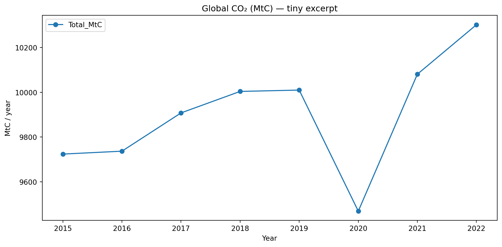
Discussion: ✏️ What comparisons are valid with such a short series? What would you add (per-capita, sector breakdown, uncertainty)?

🧰 Analysis habits we’ll use all semester

Tip

1) Inspect first (always): df.head(), df.info(), df.describe()

Tip

2) Plot early: a quick plot catches problems faster than reading 200 rows

Tip

3) Name things for meaning: co2_monthly beats df2

Tip

4) Write the takeaway in the title: make plots that explain themselves

🧯 When you’re stuck: do this in order

  1. Read the last 2 lines of the error message (that’s usually the real problem)
  2. Restart the kernel (Notebook: Kernel → Restart)
  3. Confirm the kernel/env:
    • sys.executable
    • does it point to your .venv / conda env?
  4. If it’s an import error: install into the active env
    • python -m pip install <package>
  5. Search the exact error text (copy/paste), not just “it doesn’t work”

Warning

If you ask for help, include:
(a) the code cell, (b) the full error, (c) output of sys.executable, (d) your OS.

✅ You can now…

  • Launch JupyterLab and run a notebook
  • Create and activate an environment (venv or conda)
  • Verify your setup with kernel checks (sys.executable, versions)
  • Load data, inspect it, and do basic cleaning
  • Produce at least one plot and write a one-sentence takeaway

Note

We’ll soon spend less time on tooling and more time answering questions with data.