
A Heuristic for Free Parameter Optimization
with Support Vector Machines (IJCNN 2006)
Matt Boardman and Thomas Trappenberg, Faculty of Computer Science
|
|
A Heuristic for Free Parameter Optimization |
Matt Boardman and Thomas Trappenberg, Faculty of Computer Science |
Are you looking at Support Vector Machines (SVM) to perform a classification or regression problems, but are a bit intimidated by the literature on how they work? Perhaps you would like to compare them with your own well-tuned artificial neural network (ANN), decision tree algorithm or other classifier, but are not sure how to tune an SVM for practical tasks?
We hope this page may help ... some of our group's current research is geared towards creating heuristics for blind application of SVM to practical classification and regression problems, requiring little to no knowledge on the part of the user about how the actual SVM works. A self-tuning SVM! Some MATLAB source code is provided at the bottom of this page for your enjoyment.
NEWS:
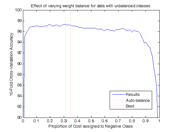
UPDATE 31/10/2006: If you're using LIBSVM, then in the case of unbalanced data you can also bias the cost values by class. During training, specify two additional options as "-w1 x" and "-w-1 y", for weighting the cost of the positive and negative classes by x and y respectively. This does seem to work well, so far we have tried this with the Wisconsin and Iris data sets and have achieved slightly higher accuracy. It's really easy to use ... as a rule of thumb, just set x and y to be the class distribution of the opposite class, ie. if you have 40% positive class and 60% negative class, use "-w1 .6" and "-w-1 .4". As a hard example, for the Wisconsin data set, the normal heuristic achieves 96.4861% 10-fold cross-validation accuracy with 52 support vectors. With this automatic class-balancing, the heuristic achieves 97.2182% with 48 support vectors: slightly better accuracy, with slightly less complexity. This rule of thumb doesn't necessarily get the best answer though; a better approach would be to use this ratio as a third dimension for the simulated annealing process. This is shown in this illustration, although it should be noted that this does not re-optimize parameters for each proportional weight value.
UPDATE 31/10/2006: There is now a version of the grid search which starts with a coarse grid and narrows in on the region of interest with increasing granularity, similar to the DOE method suggested by [Staelin, 2003] ... so far, it appears to be quite fast in comparison to a grid search but does not find the best regions in comparison to the simulated annealing method. Please email me if you're interested in the source code, I haven't added it to the package below as this code is quite new (and not very useful, except for comparison purposes!).
UPDATE 20/10/2006: We've had a successful poster presentation at Dalhousie University's Psychiatry Research Day 2006. For a neural networking audience, the most significant part of this is the novel method for selecting variables to be eliminated in backwards elimination, to reduce the number of variables for a significant increase in accuracy across all four datasets. There are few details of this method in the paper, as Dr. Trappenberg and I are currently working on a paper to discuss the approach, which we have called "empirical weight estimation." A pdf of the poster is available here:
Matthew Boardman, Sarah Ironside, Thomas Trappenberg and Penny Corkum. Support Vector Classification Shows Sleep Effects of Ritalin on Children with ADHD (Poster Presentation). Dalhousie Department of Psychiatry 16th Annual Research Day, Halifax, Nova Scotia, October 2006.
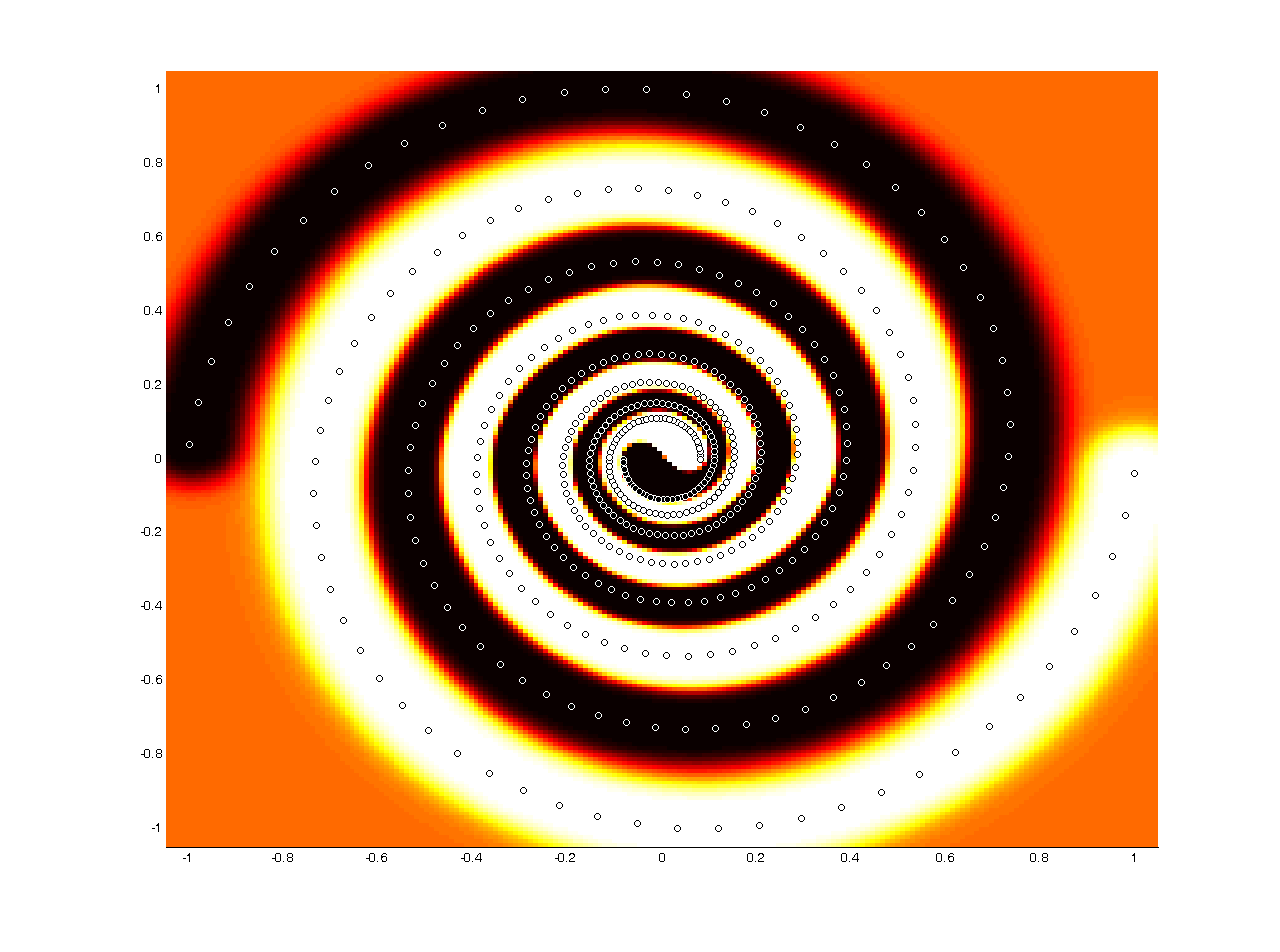
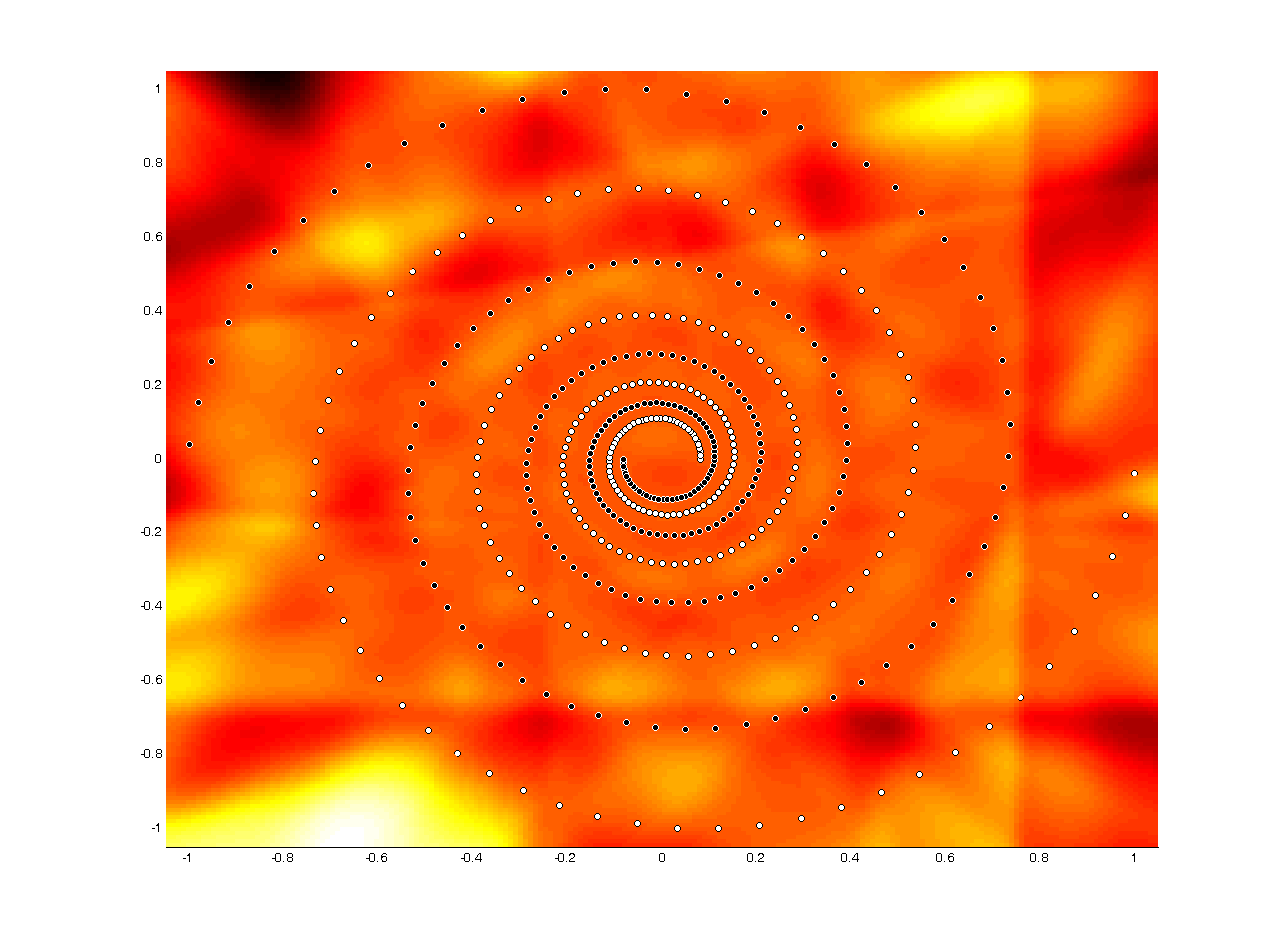
UPDATE 11/10/2006: Interested in a challenge? Think these kernel methods can't hold a candle to your own personal super-duper way-cool heavily-optimized backpropagation neural network? :) Try classifying this data set ... spiral.m. An SVM with an RBF kernel has no problem with this data, which is entirely deterministic with balanced class data, however neural networks seem to require 10s of 1000s of hidden units and hours of training to even approximate a solution. Why? We believe SVM has an advantage because with the RBF kernel it effectively has an infinite number of hidden units (an infinite-dimensional feature space). There are a few papers about this phenomenon, for example see [Suykens and Vandewalle, 1999]. The resulting decision surface that we achieved with an SVM is here, and an attempt with a Netlab MLP using 1000 hidden units with no weight decay (which should drastically overfit) is here. For an added bonus, try adding some noise to the dataset by setting n>0 in the source code above ... the SVM can still do it!
UPDATE 06/09/2006: We have found a data set in which there is a distinct increase in accuracy by removing irrelevant variables! We are currently working on a novel variable-selection method for use with statistical measures made by clinical psychiatrists here at Dal, who are using Actigraph to monitor children with ADHD. This non-linear data set, which includes several redundant measures, appears to be quite sensitive to variable selection. We will be showing the results of this research soon, please contact us for more information. We also have created a toy data set that does the same thing ... try creating a data set with twenty random Gaussian variables, where the class is positive if the sum of the first 10 variables is >5. A good algorithm should eliminate variables 11-20 as irrelevant.
|
|
|
|
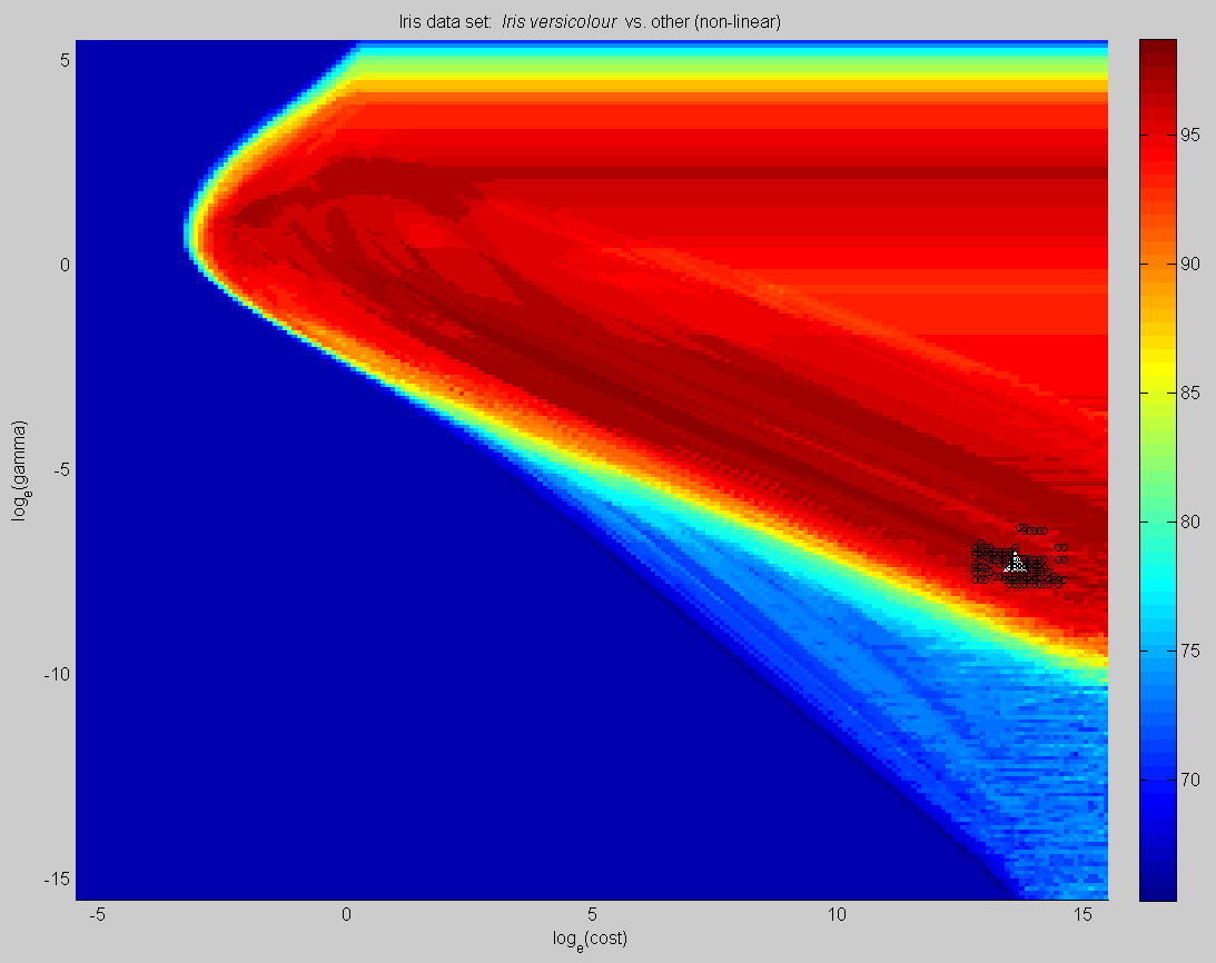
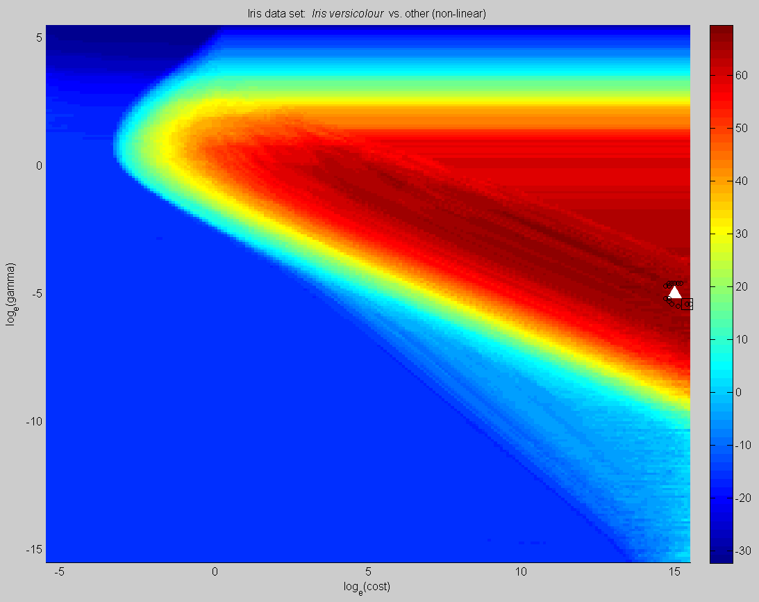
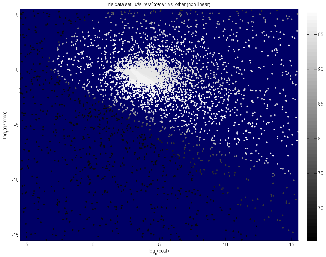
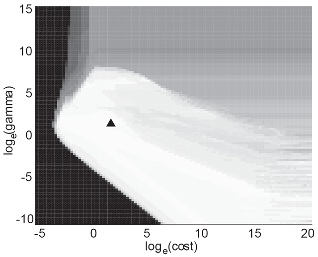
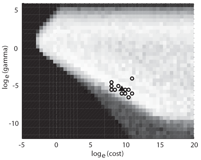
High-resolution grid search from the Iris Plant Database (UCI Machine Learning Repository). The left grid considers only 10-fold cross-validation. The centre grid considers 10-fold cross-validation and extrinsic regularization based on the number of support vectors, giving equal weight to each (lambda=1). In both diagrams, the black square is the best point found; the black circles are the group of surrounding points within a radius of 1 that have within 2% of the score of this best point; and the white triangle is the suggested point, calculated from an intensity-weighted centre of mass of this group of points. The right plot shows the same surface, with extrinsic regularization, explored by the simulated annealing heuristic: each dot corresponds to a single evaluation. All three plots find different solutions with about the same cross-validation accuracy: which is best? |
||
Our goal is not to achieve 100% cross-validation accuracy: on many finite data sets this is not achievable, due to overlapping prior distributions or misclassified samples. Rather, we will maximize the cross-validation accuracy within the bounds that are possible for a given finite data set, but importantly, we will allows some tradeoffs in accuracy for the sake of a "safer," more general solution. We especially target those cases where we have a low number of training samples, but high input dimensionality, common with medical waveform analyses such as electroretinography.
Essentially, we have three suggestions:
consider simulated annealing as a parameter search method rather than a grid search, to increase the efficiency of your search and reduce sensitivity to cross-validation noise.
consider the complexity of the resulting model, in addition to cross-validation performance, when comparing sets of parameters. We call this extrinsic regularization, as opposed to the intrinsic regularization [Tikhonov, 1963] that forms part of the SVM training algorithm.
rather than running the algorithm multiple times and using the mean or median of the results, keep the best results found during the search as you go, and calculate an intensity-weighted centre of mass of the results. We found that this results in lower volatility of the end-solution, and increased safety in the case where a subset of the training data is used to find the best parameters before training the final SVM on the full training set.
We have found excellent results by combining these elements into a working heuristic for SVM parameter optimization. A list of publications appears at the end of this page to detail some of these results.
SVM have many advantages over ANN, such as a fast and efficient training algorithm, a sparse model representation, and (most importantly here!) fewer free parameters, or hyperparameters. One of the most important advantages is the greater insensitivity to training set errors or outliers: SVM have excellent regularization capabilities, which gives them the ability to find a general solution to a problem with a minimum of available training samples.

| |
|
How do you identify a tree? |
|
Although SVM do generalize well, they are still dependent on appropriate selection of several free parameters, or hyperparameters. Inappropriate selection of these parameters can fool the SVM into giving solutions which overfit or underfit, sometimes severely, or have poor accuracy even on the training examples.
| |
|
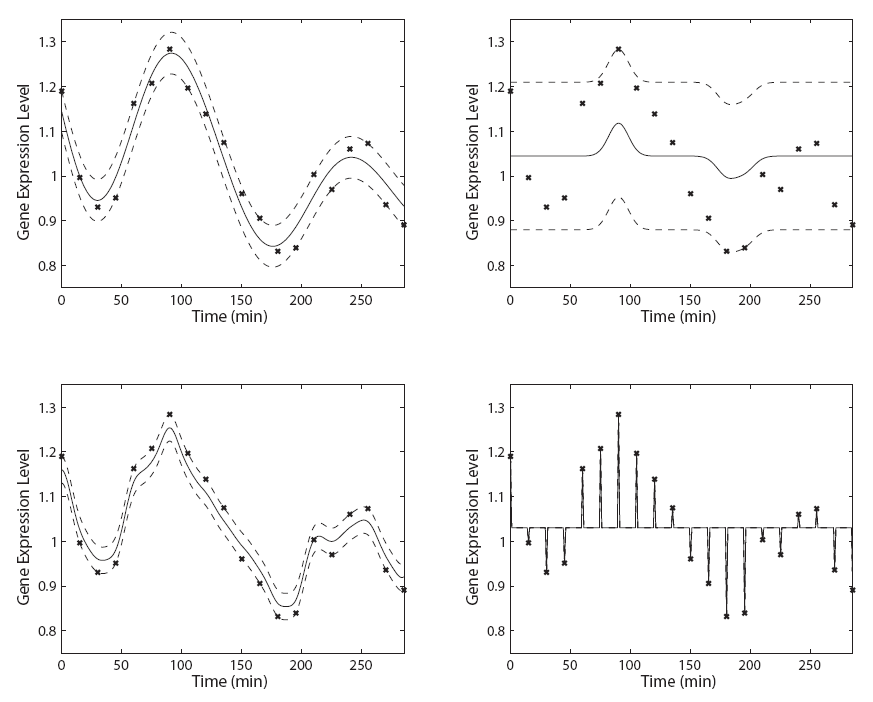
Four SVM solutions to a regression problem. The upper left case uses our heuristic, modified for noise-insensitive support vector regression. |
|
Cross-validation is one solution to the problem of overfitting, and works well. This technique randomly partitions the data into several sections, trains on all sections but one, and tests the accuracy on the remaining section of data. This process is repeated so that each partition becomes the testing partition exactly once. However, cross-validation alone is not enough! Even with cross-validation, there may be a bias of the model towards the training data.
We therefore propose what we have termed extrinsic regularization, to clearly show the relationship with the SVM's intrinsic regularization which is part of the SVM training algorithm. That is, when comparing different sets of parameters to see which gives the best-performing model, don't consider only the cross-validated accuracy or cross-validated mean squared error: consider an external factor, such as the model's complexity. An easy measure of the SVM model's complexity is the number of support vectors it uses in the model: a complex, overfitting model will have many support vectors whereas a simple, general model will have comparatively few. This technique is commonly used to regularize neural networks by considering the norm of the weight matrix as a measure of complexity [Haykin, 1999]. Other extrinsic regularization measures could be the model's performance on a separate data set drawn from the same source, or an estimate of the capacity of the model such as the VC-dimension, but we have found that the number of support vectors is a good measure of complexity and gives reasonable results in a variety of situations. Another advantage is that the number of support vectors is very easy to return directly from the resulting model, without any additional computation.
So, for each set of parameters we wish to compare, a score is computed by adding the cross-validation error on the training data (from zero to one) to the model complexity (the ratio of the number of support vectors to the number of available training samples), in the simplest case giving equal weight to each. Whichever set of parameters has the lowest score wins. Simple, right?
| |
|
A typical grid search for parameters. Brighter areas yield better cross-validation performance. |
|
This grid search works well, but the precision of the search is limited to the chosen granularity of the grid. In addition, if a third parameter is added as in the case of noise-insensitive support vector regression (epsilon-SVR), this search space becomes a cube rather than a grid, requiring many more calculations: this is the dreaded curse of dimensionality [Bellman, 1961]. Other proposed methods include a gradient descent approach [Chapelle, 1999], an iterative grid search which increases resolution to narrow in on the area of interest [Staelin, 2003], and a geometric pattern search method [Momma and Bennett, 2002]. The noise induced by the stochastic (random) partitioning in cross-validation, however, may fool such methods. In addition, the surface is fraught with local extrema which may fool gradient descent methods or limit the efficiency of geometric searches.

| |
|
A uniformly random approach (left) compared to simulated annealing (right), both with the same number of evaluations. |
|
| |
|
An intensity-weighted centre-of-mass operation, added to a grid search, moves the optimum point away from a dropoff in accuracy. |
|
Rather, we propose to keep the best points found by the algorithm (we keep all of them for display purposes, but you could keep only the best results in a moving window to save space). When the algorithm completes, the overall optimum point is selected as that with the highest score. Any surrounding points (within an arbitrary log radius) that have a performance score close to the best point (say, within 1 or 2 percent) are grouped together. Borrowing from the field of astronomy, we calculate the intensity-weighted centre of mass of these "best" points, where the intensity is simply the performance score: those points yielding higher performance will contribute more to the solution. We find that such an approach greatly reduces the volatility of the end solution point, and enhances the "safety" of the result by tending to move points away from areas of sharp dropoffs in accuracy (see the figure to the right).
Wait, enhancing the safety of the solution? What does that mean? Well, this optimization takes some time to perform. If you need a new model on a regular basis, say as part of a daily workflow, you may wish to spin your processors on more important tasks such as rebuilding database indices. So rather than optimizing the parameters each time, you can optimize your parameters once, or at least less regularly, and train the final SVM using the previously optimized set of parameters. Since we may therefore add or remove training samples, the error surface may have shifted somewhat: if your solution is near a sharp dropoff, this new finite training set may "fall" off the edge to a region of lower accuracy. Another example is where a subset of the training data is used to optimize parameters, say 100 training samples, but then the final SVM is trained using all training samples: this would save computations, but again the problem is that the new training samples might cause the classifier to fall off an edge. By using a centre of mass operation, these situations are largely prevented, which makes this heuristic more useful in practical situations.
We have expanded this heuristic to three-dimensional parameter space, to simultaneously optimize the cost parameter (C), the RBF width parameter (gamma), and the noise-insensitivity tube width (epsilon) in noise-insensitive support vector regression (epsilon-SVR). Since the dimensionality of the search space has increased, it may be advantageous to allow slower cooling in the simulated annealing algorithm: this way more of the space is evaluated. We have used this approach in two regression analyses: a predictive uncertainty in environmental modelling competition hosted by Gavin Cawley, and a semi-multivariate approach to noise-reduction and missing data imputation for periodic gene expression from microarray data based on fission yeast cell-cycle data gathered by the Wellcome Trust Sanger Institute by [Rustici et al, 2004]. Results from these analyses are found in Matthew Boardman's thesis at the bottom of this page (Chapter 5 and 6 respectively).
SVM classifiers work best when they have balanced, i.i.d. (independently and identically distributed) training data sets. So, try to ensure that you have the same number of positive samples as you have negative samples, and scale your inputs such that each dimension in the training set has more or less the same distribution: say, with values ranging from +1 to -1 and a zero mean, or with zero mean and unit variance.
What if your data set is not quite balanced? We faced this issue with the retinal electrophysiology data set in the papers below: we had six positive samples, and eight negative samples. To create a balanced training set, we selected all six positive samples, and six of the eight negative samples. Rather than selecting them at random, we selected each possible combination of six samples in turn and ran the experiment 28 times (8 choose 6 = 28). The final accuracy is then the mean of all 28 experiments. If we desire a single set of parameters to be used for subsequent experiments, we simply chose the medians of the cost and gamma parameters that were selected by tuning each experiment independently, then re-ran the experiments with these new median free parameters.
What if you have many more input dimensions than you do training samples? Well, for any other classifier or regression analysis, this would be a problem. But SVM's handle this common situation beautifully: it is, in fact, part of their design. Since the training algorithm for a non-linear SVM works in a feature space defined by the kernel, which may even be infinite-dimensional in the case of the commonly-used RBF kernel, SVM are (nearly?) immune to excessive dimensionality. They will be no more or less efficient with an excessive number of input dimensions that include irrelevant or redundant features. Depending on the nature of your problem, feature construction methods such as PCA, FFT or wavelets may well be completely irrelevant! So, at least to start with, give your SVM all possible input dimensions and let it sort out what's important during training. Later, you may find that removing some dimensions (for example, using a model-dependent sensitivity assessment method, such as [Rueda et al, 2004]) may yield higher accuracy, but this is not necessarily true (in fact, we haven't yet found a situation where feature construction or feature selection have helped to any statistically valid extent, but it's much too early to say it's never true!).
Currently, we have published a single paper based on this work, based on Matt Boardman's MCSc. thesis.
More are in progress, and will appear here or here as appropriate.
If you find an SVM useful for your work (and we hope that you do!), here are some pointers to more information that may help you to learn more about them.
www.kernel-machines.org, maintained by Alexander J. Smola and Bernhard Schölkopf.
The SVM Application List, maintained by Isabelle Guyon.
Kristen P. Bennett, Colin Campbell (2000). Support vector machines: hype or hallelujah? SIGKDD Explorations, Vol. 2, No. 2, pp. 1-13.
Christopher J. C. Burges (1998). A tutorial on support vector machines for pattern recognition. Data Mining and Knowledge Discovery, Vol. 2, No. 2, pp. 121-167, 1998.
Alexander J. Smola and Bernhard Schölkopf (2004). A tutorial on support vector regression. Statistics and Computing, Vol. 14, No. 3, pp. 199-222.
The articles and books referenced above are:
[Bellman, 1961] Richard E. Bellman, Ed. Adaptive Control Processes. Princeton University Press, 1961.
[Burges, 1998] Christopher J. C. Burges. A tutorial on support vector machines for pattern recognition. Data Mining and Knowledge Discovery, Vol. 2, No. 2, pp. 121-167, 1998.
[Chapelle, 1999] Olivier Chapelle and Vladimir N. Vapnik. Model selection for support vector machines. In S. Solla, T. Leen and K.-R. Müller, Eds., Advances in Neural Information Processing Systems, Vol. 12. MIT Press, Cambridge, MA, pp. 230-236, 1999.
[Haykin, 1999] Simon Haykin. Neural Networks: A Comprehensive Foundation, 2nd edition. Prentice-Hall, Upper Saddle River, NJ, pp. 267-277, 1999.
[Kirkpatrick et al, 1983] S. Kirkpatrick, C. D. Gelatt, Jr. and M. P. Vecchi. Optimization by simulated annealing. Science, Vol. 220, No. 4598, pp. 671-680, 1983.
[Momma and Bennett, 2002] Michinari Momma and Kristin P. Bennett. A pattern search method for model selection of support vector regression. In Proceedings of the 2nd Society for Industrial and Applied Mathematics International Conference on Data Mining, Philadelphia, PA, April 2002.
[Rueda et al, 2004] Ismael E. A. Rueda, Fabio A. Arciniegas and Mark J. Embrechts. SVM sensitivity analysis: An application to currency crises aftermaths. IEEE Transactions on Systems, Man and Cybernetics - Part A: Systems and Humans, Vol. 34, No. 3, pp. 387-398, 2004.
[Rustici et al, 2004] Gabriella Rustici, Juan Mata, Katja Kivinen, Pietro Lió, Christopher J. Penkett, Gavin Burns, Jacqueline Hayles, Alvis Brazma, Paul Nurse and Jürg Bähler. Periodic gene expression program of the fission yeast cell cycle. Nature Genetics, Vol. 36, No. 8, pp. 809-817, 2004.
[Staelin, 2003] Carl Staelin. Parameter selection for support vector machines. Technical Report HPL-2002-354 (R.1), HP Laboratories Israel, 2003.
[Suykens and Vandewalle, 1999] J.A.K. Suykens and J. Vandewalle. Least Squares Support Vector Machine Classifiers. Neural Processing Letters, Vol. 9, No. 3, pp. 293-300, 1999.
[Tikhonov, 1963] Andrei N. Tikhonov. The regularization of ill-posed problems (in Russian). Doklady Akademii Nauk USSR, Vol. SSR 153, No. 1, pp. 49-52, 1963.
This work was supported in part by the NSERC grant RGPIN 249885-03. We would also like to thank Dr. François Tremblay and Dr. Denis Falvey, Dalhousie University, for the retinal electrophysiology data analyzed in this thesis; Dr. Christian Blouin, Dalhousie University, for access to the sequence alignment data analyzed in this thesis; the genomic researchers at the Wellcome Trust Sanger Institute, Hinxton, Cambridge, for making their gene expression data publicly available; Dr. Gavin Cawley, University of East Anglia, for suggesting and holding the Predictive Uncertainty in Environmental Modelling Competition for the 2006 IEEE World Congress on Computational Intelligence; the anonymous reviewers of the IEEE, whose feedback for the published work above provided many invaluable suggestions.
The following MATLAB script files are available for download. They are provided as open source programs, with no expressed or implied warranties of any kind (see the GNU public license for more information). You are free to use or distribute the files as you like, so long as you include a reference to this page or to the IJCNN 2006 paper above as an acknowledgement of our contribution. For subsequent published works, please reference the following conference paper:
Matthew Boardman and Thomas Trappenberg (2006). A Heuristic for Free Parameter Optimization with Support Vector Machines. Proceedings of the 2006 IEEE International Joint Conference on Neural Networks (IJCNN 2006), Vancouver, BC, July 16-21, 2006, pp. 1337-1344. |
A recent version of MATLAB® is required, we performed our tests mostly on MATLAB 7.1 (R14) SP3 for Windows® and MATLAB 7.0 (R14) SP1 for Linux. Compatibility with other versions of MATLAB may also be possible.
You will also need an installed and working copy of a MATLAB-compatible Support Vector Machine implementation, such as LIBSVM (the default in the scripts above) or SVMlight. Others should also work, but you'll need to modify the scripts for the correct calling protocol.
Download now (25k) |
The following files are included in this archive:
readme.txt - this file
license.txt - a copy of the GNU General Public License
sa_svc.m - MATLAB script that implements the heuristic with simulated annealing and N-fold cross-validation (RBF kernel)
sa_svc_lin.m - MATLAB script that implements the heuristic with simulated annealing and N-fold cross-validation (Linear kernel)
sa_svc_loo.m - MATLAB script with simulated annealing and leave-one-out cross-validation (RBF kernel)
sa_svc_loo_lin.m - MATLAB script with simulated annealing and leave-one-out cross-validation (Linear kernel)
grid_svc.m - MATLAB script with a grid search and N-fold cross-validation
example.m - An example script that uses the Iris Plant Database from the UCI Machine Learning Repository
iris.mat - The training data needed for the example
Please note: a version of this heuristic used for noise-insensitive support vector regression is currently in progress. Please contact the authors above for more information. Preliminary results are available in Chapters 5 and 6 of Matthew Boardman's thesis, above.
Good luck and have fun!
| Back to top |